Fast expansions and compressions of trapped-ion chains

Abstract

We investigate the dynamics under diabatic expansions/compressions of linear ion chains. Combining a dynamical normal-mode harmonic approximation with the invariant-based inverse-engineering technique, we design protocols that minimize the final motional excitation of the ions. This can substantially reduce the transition time between high and low trap-frequency operations, potentially contributing to the development of scalable quantum information processing.

I Introduction

Trapped-ion chains provide currently a leading architecture to test and develop quantum information processing protocols 08Blatt ; reviewsim1 ; reviewsim2 . A toolbox of fundamental ion manipulations is required to implement the logical operations or simulations. This comprises procedures to control the ions’ internal (electronic) and external (motional) degrees of freedom, and also to couple them together. Such procedures should be not only feasible but also fast. Achieving high speeds is important in itself, to allow for more operations per unit time, but it is also instrumental in suppressing the effects of noise and decoherence.

Regarding motional control, a number of operations have been identified as relevant for different scalable trapped-ion quantum information architectures 02Kielpinski ; 00Cirac ; 14Monroe , including ion transport Erik ; Palmero ; Palmero2 ; Bowler ; Walther ; 13Alonso , and ion-chain splitting and recombination Bowler ; 11Home ; Kaufmann ; Ruster . These operations can be performed on single or mixed-species ion chains 13Home , allowing for sympathetic ion cooling or quantum-logic spectroscopy 05Schmidt .

The physical operation that we consider here is fast control of the motional frequencies of the trapped ions, which in the case of multiple ions leads to chain expansions and compressions. Several elementary protocols benefit from a high trap-frequency whereas others are better performed with low frequencies. Therefore, a fast transition between them without inducing final excitations is a worthwhile goal.

Operations that benefit from high motional frequencies (i.e. large potential curvature, small inter-ion distance, and small Lamb-Dicke parameters) include:

• Doppler laser cooling, since the mean phonon number is lower for tighter traps 86Stenholm ;

• any operation where a single motional normal mode (NM) of an ion chain needs to be spectrally resolved, since the NM frequency splitting is proportional to the trap curvature 11Home ;

• operations which make use of motional sidebands and whose fidelity is limited by off-resonantly driving carrier transitions on the qubit.

On the other hand, operations where a lower motional frequency is desired include:

• single-ion addressing in a multi-ion crystal;

• resolved sideband cooling, which cools at a rate proportional to the square of the Lamb-Dicke parameter 03Leibfried2 ;

• geometric phase gates 03Leibfried , which are faster for larger Lamb-Dicke parameters.

In many cases a compromise will be optimal, depending on the dominant limitations for a particular experiment.

Fast expansions/compressions without final excitation have been designed in a number of different ways Udo ; Koslof ; Masuda ; Muga ; Xi ; Review ; Adolfo . Invariant-based engineering or scaling methods Muga ; Xi were realized experimentally for a non-interacting cold-atom cloud Nice1 and a Bose-Einstein condensate Nice1 ; Nice2 . However, the methods used rely on single-particles, BEC dynamics, or equal masses, and are not directly applicable to an arbitrary interacting ion chain. We propose here a method to design trap expansions and compressions faster than adiabatically and without final motional excitation. Specifically we define dynamical normal modes similar to the ones defined for shuttling ion chains in Palmero and apply invariant-based inverse-engineering techniques by either exact or approximate methods.

We first discuss two-ion chains in Sec. II, both for ions of equal mass, and ions of different mass, and then extend the analysis in Sec. III to longer chains. In the examples only expansions of the trapping potential are considered, as compressions may be performed with the same time-evolution of the spring constant, only time-reversed.

II 2-ion chain expansion

We will deal with a one-dimensional trap containing an $N$-ion chain whose Hamiltonian in terms of the positions $\{q_{i}\}$ and momenta $\{p_{i}\}$ of the ions in the laboratory frame is

$$H=\sum_{i=1}^{N}\frac{p_{i}^{2}}{2m_{i}}+\sum_{i=1}^{N}\frac{1}{2}u_{0}(t)q_{i}^{2}+\sum_{i=1}^{N-1}\sum_{j=i+1}^{N}\frac{C_{c}}{q_{i}-q_{j}},$$ (1)

where $C_{c}=\frac{e^{2}}{4\pi\epsilon_{0}}$, with $\epsilon_{0}$ the vacuum permittivity. $u_{0}(t)$ is the common (time-dependent) spring constant that defines the oscillation frequencies $\omega_{j}(t)/(2\pi)$ for the different ions in the absence of Coulomb coupling: $u_{0}(t)=m_{1}\omega^{2}_{1}(t)=m_{2}\omega^{2}_{2}(t)=\dots=m_{N}\omega^{2}_{N}(t)$. All ions are assumed to have the same charge $e$, and be ordered as $q_{1}>q_{2}>\dots>q_{N}$, with negligible overlap of probability densities as a result of the Coulomb repulsion. The potential term $V(q_{1},q_{2})=H-\sum_{i}p_{i}^{2}/2m_{i}$ in the Hamiltonian (1) for two ions is minimal at the equilibrium points $q_{1}^{(0)}=x_{0}/2$, $q_{2}^{(0)}=-x_{0}/2$, where $x_{0}\equiv x_{0}(t)~{}=~{}2\scriptsize{\sqrt[3]{\frac{C_{c}}{4u_{0}(t)}}}$ is the equilibrium distance between the two ions. Instantaneous, mass-weighted, NM coordinates are defined by diagonalizing the matrix $V_{ij}=\frac{1}{\sqrt{m_{i}m_{j}}}\frac{\partial^{2}V}{\partial q_{i}\partial q_{j}}(q_{i}^{(0)},q_{j}^{(0)})$ Palmero . The time-dependent eigenvalues are 01Morigi

$$\lambda_{\pm}=\left(1+\frac{1}{\mu}\pm\sqrt{1-\frac{1}{\mu}+\frac{1}{\mu^{2}}}\right)\omega_{1}^{2},$$ (2)

where we have relabeled $m_{1}\rightarrow m$ and $m_{2}\rightarrow\mu m$, and omitted the explicit time dependences to avoid a cumbersome notation, i.e., $\lambda_{\pm}\equiv\lambda_{\pm}(t)$ and $\omega_{1}\equiv\omega_{1}(t)$. The time-dependent angular frequencies for each mode are

$$\Omega_{\pm}\equiv\Omega_{\pm}(t)=\sqrt{\lambda_{\pm}}=\left(1+\frac{1}{\mu}\pm\sqrt{1-\frac{1}{\mu}+\frac{1}{\mu^{2}}}\right)^{1/2}\!\!\omega_{1},$$ (3)

and the eigenvectors corresponding to these eigenvalues are $v_{\pm}=(a_{\pm},b_{\pm})^{T}$, where

$$a_{+} = \left(\frac{1}{1+\left(1-\frac{1}{\mu}-\sqrt{1-\frac{1}{\mu}+\frac{1}{\mu^{2}}}\right)^{2}\mu}\right)^{1/2},$$

$$b_{+} = \left(1-\frac{1}{\mu}-\sqrt{1-\frac{1}{\mu}+\frac{1}{\mu^{2}}}\right)\sqrt{\mu}a_{+},$$

$$a_{-} = \left(\frac{1}{1+\left(1-\frac{1}{\mu}+\sqrt{1-\frac{1}{\mu}+\frac{1}{\mu^{2}}}\right)^{2}\mu}\right)^{1/2},$$

$$b_{-} = \left(1-\frac{1}{\mu}+\sqrt{1-\frac{1}{\mu}+\frac{1}{\mu^{2}}}\right)\sqrt{\mu}a_{-}.$$ (4)

The instantaneous, dynamical normal-mode (mass weighted) coordinates are finally

$${\sf q}_{+} = a_{+}\sqrt{m}\left(q_{1}-\frac{x_{0}}{2}\right)+b_{+}\sqrt{\mu m}\left(q_{2}+\frac{x_{0}}{2}\right),$$

$${\sf q}_{-} = a_{-}\sqrt{m}\left(q_{1}-\frac{x_{0}}{2}\right)+b_{-}\sqrt{\mu m}\left(q_{2}+\frac{x_{0}}{2}\right).$$ (5)

The quantum dynamics of a state $|\psi\rangle$ governed by $H$ in the laboratory frame may be transformed into the moving frame of NM coordinates by the unitary operator

$$U=\int d{\sf q}_{+}d{\sf q}_{-}dq_{1}dq_{2}|{\sf q}_{+},{\sf q}_{-}\rangle\langle{\sf q}_{+},{\sf q}_{-}|q_{1},q_{2}\rangle\langle q_{1},q_{2}|,$$ (6)

where $\langle{\sf q}_{+},{\sf q}_{-}|q_{1},q_{2}\rangle=\delta[q_{1}-q_{1}({\sf q}_{+},{\sf q}_{-})]\delta[q_{2}-q_{2}({\sf q}_{+},{\sf q}_{-})]$. The Hamiltonian in the dynamical equation for $|\psi^{\prime}\rangle=U|\psi\rangle$ is given by

$$H^{\prime} = UHU^{\dagger}-i\hbar U(\partial_{t}U^{\dagger})=$$ (7)

$$= \sum_{\nu}\left(\frac{{\sf p}_{\nu}^{2}}{2}-{\sf p}_{0\nu}{\sf p}_{\nu}+\frac{1}{2}\Omega_{\nu}^{2}{\sf q}_{\nu}^{2}\right),$$

where cubic and higher order terms in the coordinates have been neglected, $\nu=\pm$, ${\sf p}_{\pm}$ are (mass weighted) momenta conjugate to ${\sf q}_{\pm}$, and

$${\sf p}_{0\pm}=-\dot{{\sf q}}_{\pm}=\frac{2}{3}(-a_{\pm}\sqrt{m_{1}}+b_{\pm}\sqrt{m_{2}})\sqrt[3]{\frac{C_{c}}{4m_{1}\omega_{1}^{5}}}\dot{\omega}_{1}$$ (8)

are functions of time with the same dimensions as the mass weighted momenta. They appear because of the time dependence of the NM coordinates through $x_{0}$, which is a function of $\omega_{1}(t)$. These ${\sf p}_{0\pm}$ functions act as momentum shifts in a further unitary transformation which suppresses the terms linear in ${\sf p}_{\pm}$,

$$\mathcal{U} = e^{-i({\sf p}_{0+}{\sf q}_{+}+{\sf p}_{0-}{\sf q}_{-})/\hbar},$$

$$|\psi^{\prime\prime}\rangle = \mathcal{U}|\psi^{\prime}\rangle,$$

$$H^{\prime\prime} = \mathcal{U}H^{\prime}\mathcal{U}^{\dagger}-i\hbar\mathcal{U}(\partial_{t}\mathcal{U}^{\dagger})=$$ (9)

$$= \sum_{\nu}\left[\frac{{\sf p}_{\nu}^{2}}{2}+\frac{1}{2}\Omega_{\nu}\left({\sf q}_{\nu}+\frac{\dot{{\sf p}}_{0\nu}}{\Omega_{\nu}^{2}}\right)^{2}\right].$$

This Hamiltonian corresponds to two effective harmonic oscillators with time-dependent frequencies and a time-dependent moving center. Note that the “motion” of the harmonic oscillators is in the normal-mode-coordinate space, and that the actual center of the external trap in the laboratory frame is fixed. According to Eqs. (3) and (8) both the NM harmonic oscillators’ centers ($-{\dot{{\sf p}}_{0\pm}}/{\Omega_{\pm}^{2}}$) and the frequencies ($\Omega_{\pm}$) depend on $\omega_{1}(t)$. This is important as, to solve the dynamics for given $\omega_{1}(t)$, the oscillators are effectively independent. However, from an inverse-engineering perspective, their time-dependent parameters cannot be designed independently. This “coupling” is here more involved than for the transport of two ions in a rigidly moving harmonic trap Palmero , where ${\sf p}_{0\pm}(t)$ take different forms which depend on the trap position but not on the trap frequency. A different approach is thus required.

The Lewis-Riesenfeld invariants LR of the two oscillators are

$$I_{\pm} = \frac{1}{2}[\rho_{\pm}({\sf p}_{\pm}-\dot{\alpha}_{\pm})-\dot{\rho}_{\pm}({\sf q}_{\pm}-\alpha_{\pm})]^{2}$$ (10)

$$+ \frac{1}{2}\Omega_{0\pm}^{2}\left(\frac{{\sf q}_{\pm}-\alpha_{\pm}}{\rho_{\pm}}\right)^{2},$$

where $\Omega_{0\pm}=\Omega_{\pm}(0)$. The invariants depend on the auxiliary functions $\rho_{\pm}$ (scaling factors of the expansion modes) and $\alpha_{\pm}$ (mass scaled centers of the dynamical modes of the invariant). They satisfy the auxiliary (Ermakov and Newton) equations

$$\ddot{\rho}_{\pm}+\Omega_{\pm}^{2}\rho_{\pm}=\frac{\Omega_{0\pm}^{2}}{\rho_{\pm}^{3}},$$ (11)

$$\ddot{\alpha}_{\pm}+\Omega_{\pm}^{2}\alpha_{\pm}=\dot{{\sf p}}_{0\pm}.$$ (12)

Dynamical expansion modes $|\psi_{n\pm}^{\prime\prime}\rangle$ (not to be confused with normal modes) may be found. These are exact time-dependent solutions of the Schrödinger equation and also instantaneous eigenstates of the invariant Erik ,

$$\langle{\sf q}_{\pm}|\psi^{\prime\prime}_{n\pm}\rangle=e^{\frac{i}{\hbar}\left[\frac{\dot{\rho}_{\pm}{\sf q}_{\pm}^{2}}{2\rho_{\pm}}+(\dot{\alpha}_{\pm}\rho_{\pm}-\alpha_{\pm}\dot{\rho}_{\pm})\frac{{\sf q}_{\pm}}{\rho_{\pm}}\right]}\frac{\Phi_{n}(\sigma_{\pm})}{\rho_{\pm}^{1/2}},$$ (13)

where $\sigma_{\pm}=\frac{{\sf q}_{\pm}-\alpha_{\pm}}{\rho_{\pm}}$ and $\Phi_{n}(\sigma_{\pm})$ are the eigenfunctions of the static harmonic oscillator at time $t=0$. Within the harmonic approximation the NM wave functions $|\psi^{\prime\prime}_{\pm}\rangle$ evolve independently with $H^{\prime\prime}$. They may be written as combinations of the expansion modes, $|\psi^{\prime\prime}_{\pm}(t)\rangle=\sum_{n}c_{n\pm}|\psi^{\prime\prime}_{n\pm}\rangle$ with normalized constant amplitudes. The average energies of the $n$-th expansion mode for two NM are

$$E^{\prime\prime}_{n\pm} = \langle\psi^{\prime\prime}_{n\pm}|H^{\prime\prime}|\psi^{\prime\prime}_{n\pm}\rangle$$ (14)

$$= \frac{(2n+1)\hbar}{4\Omega_{0\pm}}\left(\dot{\rho}_{\pm}^{2}+\Omega_{\pm}^{2}\rho_{\pm}^{2}+\frac{\Omega_{0\pm}^{2}}{\rho_{\pm}^{2}}\right)$$

$$+ \frac{1}{2}\dot{\alpha}_{\pm}^{2}+\frac{1}{2}\Omega_{\pm}^{2}(\alpha_{\pm}-\dot{{\sf p}}_{0\pm}/\Omega_{0\pm}^{2})^{2}.$$

In numerical examples the initial ground state is, in the harmonic approximation, of the form $|\psi^{\prime\prime}_{0+}(0)\rangle|\psi^{\prime\prime}_{0-}(0)\rangle$, so the time dependent energy is given by $E^{\prime\prime}(t)=E^{\prime\prime}_{0+}+E^{\prime\prime}_{0-}$. Note that if we impose both unitary operators $U(t)$ and ${\cal U}(t)$ to be 1 at $t=0$ and $t_{f}$, the transformed wave function $|\psi^{\prime\prime}\rangle$ and the laboratory wave function $|\psi\rangle$ will be the same at both these times and the energy $E^{\prime\prime}(t=0,t_{f})$ will be the same as the laboratory-frame energy. Both unitary transformations satisfy this provided that $\dot{\omega}_{1}(t_{b})=0$, where $t_{b}=0,t_{f}$, as long as the quadratic approximation in the Hamiltonian (II) is valid.

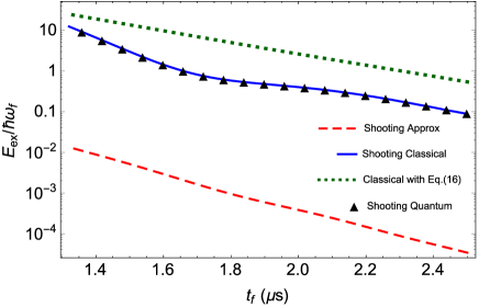
Figure 1: (Color online) Final excitation energy at $t_{f}$ for the expansion of two ⁴⁰Ca⁺ ions, with respect to the final ground state (quantum) or the final equilibrium energy (classical). The initial state is the ground state (quantum) or the equilibrium state (classical) for the initial trap. The dashed red line is the excitation in the harmonic approximation, using Eq. (14) for the NM energies, with the protocol obtained by the shooting method; the solid blue line (classical) and black triangles (quantum) are for the same protocol but with the dynamics driven by the full Hamiltonian (1). The dotted green line is for the protocol (16) with the full Hamiltonian. The parameters used are $\omega_{0}/(2\pi)=1.2$ MHz and $\gamma^{2}=3$.

For a single harmonic oscillator without the independent term in Eq. (12), i.e. with a fixed center, the frequency in a trap expansion was already inverse engineered in Xi . For this case we can use the same notation as before but no subindices for the auxiliary functions. $\alpha$ is zero for all times, and in the Ermakov equation the conditions $\rho(0)=1$, $\rho(t_{f})=\gamma=\sqrt{\omega_{0}/\omega_{f}}$, and $\dot{\rho}(t_{b})=\ddot{\rho}(t_{b})=0$, suffice to avoid any excitation (since $[H(t_{b}),I(t_{b})]=0$) and ensure continuity of the oscillator frequency. Any interpolated function $\rho(t)$ satisfying these conditions provides a valid $\Omega(t)$. Similarly, in harmonic transport of an ion (with the trap moving rigidly from 0 to $d$ with a constant frequency Erik ) the auxiliary equation for $\rho$ becomes trivially satisfied by $\rho=1$ and, to avoid excitations and ensure continuity, $\alpha$ may be any interpolated function satisfying $\alpha(0)=0$, $\alpha(t_{f})=d$, $\dot{\alpha}(t_{b})=\ddot{\alpha}(t_{b})=0$ Erik . Instead of these simpler settings, when inverse engineering the expansion of the ion chain the auxiliary equations (11) are non-trivially coupled and have to be solved consistently with Eq. (12), since $\Omega_{\pm}$ and ${\sf p}_{0\pm}$ are functions of the same frequency $\omega_{1}$. In other words, only interpolated auxiliary functions $\rho_{\pm}(t)$, $\alpha_{\pm}(t)$ consistent with the same $\omega_{1}(t)$ are valid.

For both NM, we impose for Eq. (11) the boundary conditions (BC) $\rho_{\pm}(0)=1$, $\rho_{\pm}(t_{f})=\gamma$, $\dot{\rho}_{\pm}(t_{b})=\ddot{\rho}_{\pm}(t_{b})=0$. Here $\omega_{0}=\omega_{1}(0)$ and $\omega_{f}=\omega_{1}(t_{f})$. The BC for the second set of equations are $\alpha_{\pm}(t_{b})=\dot{\alpha}_{\pm}(t_{b})=\ddot{\alpha}_{\pm}(t_{b})=0$. Eq. (12) with Eq. (8) implies that at the boundaries we must have $\frac{5}{3}\frac{\dot{\omega}_{1}^{2}(t_{b})}{w_{1}(t_{b})}-\ddot{\omega}_{1}(t_{b})=0$. This is satisfied by imposing $\dot{\omega}_{1}(t_{b})=0$, $\ddot{\omega}_{1}(t_{b})=0$. Substituting these conditions in Eq. (11) we finally get the extra BC $\rho_{\pm}^{(3)}(t_{b})=\rho_{\pm}^{(4)}(t_{b})=0$.

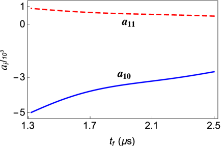
Figure 2: (Color online) The values of the optimizing free parameters in the two-ion expansion $a_{10}$ (solid blue line) and $a_{11}$ (dashed red line) in the expansion of two ⁴⁰Ca⁺ ions starting in the ground state. $\omega_{0}/(2\pi)=1.2$ MHz, $\gamma^{2}=3$.

To engineer the auxiliary functions we proceed as follows: first we design $\rho_{-}(t)$ so as to satisfy the 10 BC for $\rho_{-}(t_{b})$ and their derivatives. They could be satisfied with a ninth-order polynomial, but we shall use higher order polynomials so that free parameters are left. These may be chosen to satisfy the equations for the remaining BC for $\alpha_{\pm}$ and $\rho_{+}$. $\omega_{1}(t)$ is deduced from the polynomial using Eq. (11) so it becomes a function of the free parameters. There are different ways to fix the free parameters so as to satisfy the remaining BC and design the other auxiliary functions. In practice we have used a shooting method shooting . The BC used for the shooting are $\alpha_{\pm}(0)=\dot{\alpha}_{\pm}(0)=\dot{\rho}_{+}=0$ and $\rho_{+}(0)=1$. Note that if $\alpha_{\pm}(t_{b})=0$, then $\ddot{\alpha}_{\pm}(t_{b})=0$ since we impose $\dot{\omega}_{1}(t_{b})=\ddot{\omega}_{1}(t_{b})=0$. The differential equations (11) for $\rho_{+}(t)$ and (12) for $\alpha_{\pm}$ are now solved forward in time.

In the following one must distinguish between single-species and mixed-species ion chains. A consequence of having equal mass ions is that $\alpha_{-}(t)$ is 0 at all times (because the ion chain is symmetric, and thus the center of mass remains static) so we only have to design the three auxiliary functions $\rho_{\pm}(t)$ and $\alpha_{+}(t)$. When both ions are of different species, the chain is not symmetric anymore, so we also need to design $\alpha_{-}$ taking into account its BC.

The MatLab function ‘fminsearch’ shooting is used to find the free parameters that minimize the total final energy for the approximate Hamiltonian, $E^{\prime\prime}_{0+}(t_{f})+E^{\prime\prime}_{0-}(t_{f})$, see Eq. (14). For equal mass ions, an 11-th order polynomial $\rho_{-}(t)=\sum_{n=0}^{11}a_{n}t^{n}/t_{f}^{n}$, i.e. two free parameters, is enough to achieve negligible excitation in a range of times for which the harmonic approximation is valid. Only two free parameters are needed to satisfy the BC $\alpha_{+}(t_{f})=\dot{\alpha}_{+}(t_{f})=0$, whereas $\rho_{+}(t_{f})=\gamma$ is also nearly satisfied for all values of these free parameters because the evolution of this scaling factor is close to being adiabatic. $\omega_{1}(t)$ is then a function of the free parameters $a_{10},a_{11}$. Fig. 1 depicts the final excitation energy for optimized parameters in the harmonic approximation, using Eq. (II), and with the full Hamiltonian (1), whereas in Fig. 2 the values of the optimizing free parameters are represented. The quantum simulations (triangles in Fig. 1) are performed starting from the ground state of the Hamiltonian (1) at $t=0$, which is calculated numerically. For the corresponding classical simulations we solve Hamilton’s equations for the two ions in the laboratory frame with Eq. (1): the excitation energy is calculated as the total energy minus the minimal energy of the ions in equilibrium. The initial conditions correspond as well to the ions in equilibrium. As the potential is effectively nearly harmonic and the evolution of wave packet’s width ($\rho_{\pm}$) is close to being adiabatic, the classical excitation energy reproduces accurately the quantum excitation energy, as demonstrated in Fig. 1. Quantum calculations are very demanding, in particular with three or more ions, so that we shall only perform classical calculations from now on.

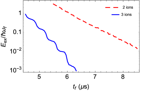
Figure 3: (Color online) Final excitation energy for the expansion of a ⁹Be⁺-⁴⁰Ca⁺ ion chain (solid blue line) and a ⁹Be⁺-⁴⁰Ca⁺-⁹Be⁺ chain (dashed red line) starting in the equilibrium configuration. The protocols are optimized with four (for ⁹Be⁺-⁴⁰Ca⁺) and two (for ⁹Be⁺-⁴⁰Ca⁺-⁹Be⁺) free parameters, see the main text. $\omega_{0}/(2\pi)=1.2$ MHz, $\gamma^{2}=3$.

For two different ions, we use a 13-th order polynomial $\rho_{-}(t)=\sum_{n=0}^{13}a_{n}t^{n}/t_{f}^{n}$, which is enough to nearly satisfy $\alpha_{\pm}(t_{f})=\dot{\alpha}_{\pm}(t_{f})=0$ and $\rho_{+}(t_{f})=\gamma$ by finding suitable values for the four free parameters $a_{10-13}$. As before, $\rho_{+}(t_{f})=\gamma$ is nearly satisfied without any special design. Fig. 3 shows the final excitation for a chain of two different ions. The excitation is higher than for equal masses. Both for the equal mass and different mass expansions, the (exact) excitation energy increases at short times, where the quadratic approximation to set the NM Hamiltonians fails, see Figs. 1 and 3. Further simulations indicate that the larger the ratio between the masses, the higher the excitation.

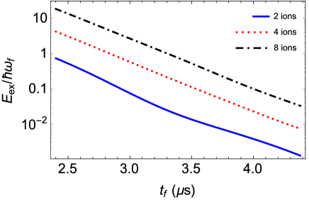
Figure 4: (Color online) Final excitation vs. final times for expansions of two equal ions (solid blue line), 4 equal ions (red dots) and 8 equal ions (dash-dotted black line). The simulations are performed according to the approximate protocol in Eq. (16) and by solving the classical equations of motion for ⁴⁰Ca⁺ ions. The initial ion chain is at equilibrium. $\omega_{0}/(2\pi)=1.2$ MHz, $\gamma^{2}=3$.

A less accurate, approximate treatment is based on the simpler polynomial ansatz $\rho_{-}=\sum_{n=0}^{9}a_{n}t^{n}$ without free parameters,

$$\rho_{-} = 126(\gamma-1)s^{5}-420(\gamma-1)s^{6}+540(\gamma-1)s^{7}$$ (15)

$$- 315(\gamma-1)s^{8}+70(\gamma-1)s^{9}+1,$$

$s=t/t_{f}$. While the BC of $\rho_{+}$ and $\alpha_{\pm}$ are in general not accounted for exactly, an advantage of this procedure is that there is no need to perform any numerical minimization. This is useful to generalize the method for larger ion chains. For equal masses, both $\alpha_{-}=0$ and $\rho_{-}(t)$ are correctly designed, so that the center of mass is not excited. From Eq. (11), $\omega_{1}(t)$ is given by

$$\omega_{1}=\sqrt{\frac{\omega_{0}^{2}}{\rho_{-}^{4}}-\frac{\ddot{\rho}_{-}}{A_{-}^{2}\rho_{-}}},$$ (16)

where $A_{-}=\Omega_{-}/\omega_{1}$ is a constant, see Eq. (3). In Fig. 1 we compare the performance of this approximate protocol and the one that satisfies all the BC in the two-equal-ion expansion.

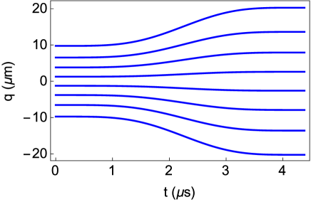
Figure 5: (Color online) Classical trajectories of eight expanding ⁴⁰Ca⁺ ions. The evolution is performed according to Eq. (16). $\omega_{0}/(2\pi)=1.2$ MHz, $\gamma^{2}=3$, $t_{f}=4.4$ $\mu$s.

III N-ion chain expansion

We now proceed to extend the results in the previous section to larger ion chains governed by the Hamiltonian (1). The equilibrium positions can be written in the form James

$$q_{i}^{(0)}(t)=l(t)u_{i},$$ (17)

where

$$l^{3}(t)=\frac{C_{c}}{u_{0}(t)}$$ (18)

and the $u_{i}$ are the solutions of the system

$$u_{i}-\sum_{j=1}^{i-1}\frac{1}{(u_{i}-u_{j})^{2}}+\sum_{j=i+1}^{N}\frac{1}{(u_{i}-u_{j})^{2}}=0.$$ (19)

The NM coordinates are thus defined as 13Home

$${\sf q}_{\nu}=\sum_{i}a_{\nu i}\sqrt{m_{j}}(q_{i}-q_{i}^{(0)}),$$ (20)

where the NM subscript $\nu$ runs now from $1$ to $N$. Conventionally the $\nu$ are ordered from the lowest to the highest frequency James . As for two ions we define $V(q_{1},q_{2},q_{3},...,q_{N})$ as the coordinate-dependent part of the Hamiltonian (1). The $a_{\nu i}$ are the components of the $\nu$-th eigenvector of the symmetric matrix $V_{ij}~{}=~{}\frac{1}{\sqrt{m_{i}m_{j}}}\frac{\partial^{2}V}{\partial q_{i}\partial q_{j}}(q_{i}^{(0)},q_{j}^{(0)})$, that, together with the eigenvalues $\lambda_{\nu}=\Omega_{\nu}^{2}$ will usually be determined numerically James . They are normalized as $\sum_{i}a_{\nu i}^{2}=1$. As $u_{0}$ is common to all ions, it can be shown that $\Omega_{\nu}(t)=A_{\nu}\omega_{1}(t)$, where $A_{\nu}$ is a constant.

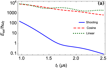
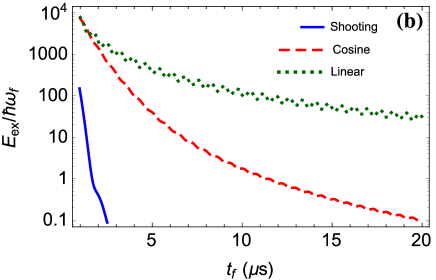
Figure 6: (Color online) Comparison of final excitation quanta (classical simulation as in Fig. 1) vs final time in the expansion of 2 ⁴⁰Ca⁺ ions following the shooting protocol (solid blue), linear protocol in Eq. (24) (dotted green) and cosine protocol in Eq. (25) (dashed red). In a) we plot in logarithmic scale up to times where only the shooting protocol reaches the level of $0.1$ excitation quanta. In b) we extend the analysis up to longer final times, so that the best of the cosine protocol reaches also 0.1 final excitation quanta. $\omega_{0}/(2\pi)=1.2$ MHz, $\gamma^{2}=3$.

Generalizing the steps leading to Eq. (7), the Hamiltonian in a NM frame up to quadratic terms becomes

$$H^{\prime}=\sum_{\nu}\bigg{[}\frac{{\sf p}_{\nu}^{2}}{2}+\frac{1}{2}\Omega_{\nu}^{2}{\sf q}_{\nu}^{2}+{\sf p}_{0\nu}{\sf p}_{\nu}\bigg{]},$$ (21)

where the ${\sf p}_{\nu}$ are momenta conjugate to the ${\sf q}_{\nu}$, and ${\sf p}_{0\nu}=-\sum_{i}a_{\nu i}\sqrt{m_{i}}\dot{q}_{i}^{(0)}$. As for two ions, all the ${\sf p}_{0\nu}$ are proportional to $\dot{\omega}_{1}/\omega_{1}^{5/3}$. We now apply the unitary transformation $\mathcal{U}=e^{-i\sum_{\nu}{\sf p}_{0\nu}{\sf q}_{\nu}/\hbar}$ and find the effective Hamiltonian

$$H^{\prime\prime}=\sum_{\nu}\bigg{[}\frac{{\sf p}_{\nu}^{2}}{2}+\frac{1}{2}\Omega_{\nu}^{2}\left({\sf q}_{\nu}+\frac{\dot{{\sf p}}_{0\nu}}{\Omega_{+}^{2}}\right)^{2}\bigg{]}.$$ (22)

This Hamiltonian is similar to the one for two ions (II). The corresponding set of auxiliary equations is also similar to Eqs. (11) and (12),

$$\ddot{\rho}_{\nu}+\Omega_{\nu}^{2}\rho_{\nu}=\frac{\Omega_{0\nu}^{2}}{\rho_{\nu}^{3}},$$

$$\ddot{\alpha}_{\nu}+\Omega_{\nu}^{2}\alpha=\dot{{\sf p}}_{0\nu}.$$ (23)

The BC for inverse engineering read $\rho_{\nu}(0)=1$, $\rho_{\nu}(t_{f})=\gamma$, $\dot{\rho}_{\nu}(t_{b})=\ddot{\rho}_{\nu}(t_{b})=0$, $\alpha_{\nu}(t_{b})=\dot{\alpha}_{\nu}(t_{b})=\ddot{\alpha}_{\nu}(t_{b})=0$. When introducing the BC for the $\alpha_{\nu}$ in the set of Newton’s equations, we get from all of them the same condition $\frac{\dot{\omega}_{1}(t_{b})}{\omega_{1}(t_{b})}+\ddot{\omega}_{1}(t_{b})=0$, which is satisfied for $\dot{\omega}_{1}(t_{b})=\ddot{\omega}_{1}(t_{b})=0$.

Fig. 4 depicts the excitation for expansions of single-species ion-chains, with approximate (non-optimized) protocols that use Eqs. (15) and (16), but with the lowest frequency mode, $\nu=1$, instead of the $minus$ $(-)$ mode. The longer the chain the lower the fidelity of the protocol, as more terms are neglected in the NM approximation and more boundary conditions are disregarded. However, the protocol still provides little excitation at long enough final times in the most demanding simulation that we examined, $N=8$. Fig. 5 shows the position of the ions, and the trap frequency along the evolution time for the eight-ion chain, ending up with a separation between ions twice as large as the initial one, in times shorter than 4 $\mu$s (Fig. 4) without any significant final excitation.

In Fig. 3 the excitation for an expansion of the two-species chain ⁹Be⁺-⁴⁰Ca⁺-⁹Be⁺ is depicted. The minimization technique was used with two free parameters, that is, with an 11-th order polynomial ansatz for $\rho_{\nu=1}(t)$. The excitation is smaller than for the shorter chain ⁹Be⁺-⁴⁰Ca⁺ (with a 13-th order polynomial for $\rho_{-}$) due to the symmetry in the three-ion chain, which leaves two of the NM static and unexcited.

IV Discussion

We have designed fast diabatic protocols for the time dependence of the trap frequency that suppress the final excitation of different ion-chain expansions or compressions. Unlike the simpler single-ion expansion Xi , the inverse design problem of the trap frequency for an ion chain involves coupled Newton and Ermakov equations for each dynamical normal mode. We found ways to deal with this inverse problem by applying a shooting technique in the most accurate protocols, and effective, simplifying approximations.

These protocols work for process times for which the quadratic approximation for the Hamiltonian is valid. Longer and more asymmetric chains need larger times than shorter and symmetrical ones. The examples show that these times are compatible with current quantum information protocols, so many processes may benefit by the described trap frequency time dependencies.

The designed protocols provide a considerable improvement in final time and excitation energy with respect to simple, naive protocols. For the expansion of two ⁴⁰Ca⁺ considered in Fig. 1 we compare in Fig. 6 the excitation energy of the shooting protocol with two simple protocols that drive the frequency $\omega_{1}$ linearly,

$$\omega_{1}(t)=\omega_{0}+\frac{\omega_{f}-\omega_{0}}{t_{f}}t,$$ (24)

and following a cosine function,

$$\omega_{1}(t)=\frac{\omega_{0}+\omega_{f}}{2}+\frac{\omega_{0}-\omega_{f}}{2}\cos\left(\frac{\pi t}{t_{f}}\right).$$ (25)

The simulations are classical, as described in Sec. II. Fig. 6 (a) compares the excitations at short times. For $t_{f}\sim 2.5$ $\mu$s, the shooting protocol reaches a low excitation of 0.1 vibrational quanta, four orders of magnitude smaller than the excitations due to the simple methods. In Fig. 6 (b) the excitations are represented for longer protocol times. The smoother cosine protocol behaves better than the linear one and finally reaches an excitation of approximately 0.1 quanta for $t_{f}\sim 20$ $\mu$s.

References

- (1) R. Blatt and C. F. Roos, Nat. Phys 8, 277 (2012).
- (2) S. Korenblit, D. Kafri, W. C. Campbell, R. Islam, E. E. Edwards, Z.-X. Gong, G.-D. Lin, L.-M. Duan, J. Kim, K. Kim, and C. Monroe, New J. Phys. 14, 095024 (2012).
- (3) R. Blatt, and D. J. Wineland, Nature 453, 1008 (2008).
- (4) D. Kielpinski, C. Monroe, and D. J. Wineland, Nature 417, 709 (2002).
- (5) J. I. Cirac, and P. Zoller, Nature 404, 579 (2000).
- (6) C. Monroe, R. Raussendorf, A. Ruthven, K. R. Brown, P. Maunz, L. M. Duan, and J. Kim, Phys Rev. A 89, 022317 (2014).
- (7) E. Torrontegui, S. Ibáñez, X. Chen, A. Ruschhaupt, D. Guéry-Odelin, and J. G. Muga, Phys. Rev. A 83, 013415 (2011).
- (8) M. Palmero, E. Torrontegui, D. Guéry-Odelin, and J. G. Muga, Phys. Rev. A 88, 053423 (2013).
- (9) M. Palmero, R. Bowler, J. P. Gaebler, D. Leibfried, and J. G. Muga, Phys. Rev. A 90, 053408 (2014).
- (10) R. Bowler, J. Gaebler, Y. Lin, T. R. Tan, D. Hanneke, J. D. Jost, J. P. Home, D. Leibfried, and D. J. Wineland, Phys. Rev. Lett. 109, 080502 (2012).
- (11) A. Walther, F. Ziesel, T. Ruster, S.T. Dawkins, K. Ott, M. Hettrich, K. Singer, F. Schmidt-Kaler, and U. Poschinger, Phys. Rev. Lett. 109, 080501 (2012).
- (12) J. Alonso. F. M. Leupold, B. C. Keitch and J. P. Home, New J. Phys. 15, 023001 (2013).
- (13) J. P. Home, D. Hanneke, J. D. Jost, D. Leibfried, D. J. Wineland, New J. Phys. 13, 073026 (2011).
- (14) H. Kaufmann, T. Ruster, C. T. Schmiegelow, F. Schmidt-Kaler, and U. G. Poschinger, New J. Phys. 16, 073012 (2014).
- (15) T. Ruster, C. Warschburger, H. Kaufmann, C. T. Schmiegelow, A. Walther, M. Hettrich, A. Pfister, V. Kaushal, F. Schmidt-Kaler, and U. G. Poschinger, Phys. Rev. A 90, 033410 (2014).
- (16) J. P. Home, Adv. At. Mol. Opt. Phys. 62, 231 (2013).
- (17) P. O. Schmidt, T. Rosenband, C. Langer, W. M. Itano, J. C. Bergquist, D. J. Wineland, Science 309, 749-752 (2005).
- (18) S. Stenholm, Rev. Mod. Phys. 58, 699 (2009).
- (19) D. Leibfried, R. Blatt, C. Monroe, and D. J. Wineland, Rev. Mod. Phys. 75, 281 (2003).
- (20) D. Leibfried, B. DeMarco, V. Meyer, D. Lucas, M. Barrett, J. Britton, W. M. Itano, B. Jelenkovic, C. Langer, T. Rosenband, and D. J. Wineland, Nature 422, 412 (2003).
- (21) T. Schmiedl, E. Dieterich, P.-S. Dieterich and U. Seifert, J. Stat. Mech. P07013 (2009).
- (22) S. Masuda and K. Nakamura, Proc. R. Soc. A 466, 1135 (2010).
- (23) P. Salamon, K.H. Hoffmann, Y. Rezek, and R. Kosloff, Phys. Chem. Chem. Phys. 11, 1027 (2009).
- (24) J. G. Muga, X. Chen, A. Ruschhaupt, and D. Guéry-Odelin, J. Phys. B: At. Mol. Opt. Phys. 42, 241001 (2009).
- (25) X. Chen, A. Ruschhaupt, S. Schmidt, A. del Campo, D. Guéry-Odelin, and J. G. Muga, Phys. Rev. Lett. 104, 063002 (2010).
- (26) E. Torrontegui, S. Ibáñez, S. Martínez-Garaot, M. Modugno, A. del Campo, D. Guéry-Odelin, A. Ruschhaupt, Xi Chen, and J.G. Muga, Adv. At. Mol. Opt. Phy. 62, 117 (2013).
- (27) A. del Campo and M. G. Boshier, Sci. Rep. 2, 648 (2012).
- (28) J. F. Schaff, X. L. Song, P. Vignolo, and G. Labeyrie, Phys. Rev. A 82 033430 (2010); Phys. Rev. A 83, 059911(E) (2011) .
- (29) J. F. Schaff, X. L. Song, P. Capuzzi, P. Vignolo, and G. Labeyrie, EPL 93, 23001 (2011).
- (30) G. Morigi and H. Walther, Eur. Phys. J. D 13, 261 (2001).
- (31) H. R. Lewis, and W. B. Riesenfeld, J. Math. Phys. 10, 1458 (1969).
- (32) J. C. Lagarias, J. A. Reeds, M. H. Wright, and P. E. Wright, SIAM Journal of Optimization, 9, 112 (1998).
- (33) D. F. V. James, Appl. Phys. B 66 181 (1998).