Correlations and synchronization in a Bose-Fermi mixture

Abstract

We study a Bose-Fermi mixture within the framework of the mean-field theory, including three possible regimes for the fermionic species: fully polarized, BCS, and unitarity. Starting from the 3D description and using the variational approximation (VA), we derive 1D and 2D systems of equations, under the corresponding confining potentials. This method produces a pair of nonlinear Schrödinger (NLS) equations coupled to algebraic equations for the transverse widths of the confined state. The equations incorporate interactions between atoms of the same species and between the species, assuming that the latter can be manipulated by means of the Feshbach resonance (FR). As an application, we explore spatial density correlations in the ground state (GS) between the species, concluding that they strongly depend on the sign and strength of the inter-species interaction. Also studied are the dynamics of the mixture in a vicinity of the GS and the corresponding spatiotemporal inter-species correlation. The correlations are strongly affected by the fermionic component, featuring the greatest variation in the unitary regime. Results produced by the VA are verified by comparison with full numerical solutions.

Keywords: Article preparation, IOP journals

1 Introduction

Cold atom gases trapped in magneto-optical potentials have tremendously extended the range of experimental possibilities in condensed-matter physics. The possibility of controlling the intensity of the interactions, the depth of the trapping potential lattices, and their geometry enables emulating a broad variety of solid-state settings and the creation of novel states of the quantum matter [1]-[8].

In this context, a great variety of experimental and theoretical studies were stimulated by the possibility of mixing degenerate bosonic and fermionic gases. The first experimental works on Bose-Fermi mixtures (BFMs) were conducted with lithium isotopes [9, 10], which was a precursor to the study of new combinations, such as ¹⁷⁴Yb-⁶Li [11] and ⁸⁷Rb-⁴⁰K [12]. Particular attention has been paid to heavy-atom mixtures, e.g., ⁸⁷Sr-⁸⁴Sr [13] isotopes with a large nuclear spin, that have been proposed as prototypes for handling the quantum information. One of important points of the work in this direction is the use of Feshbach resonances (FRs) in the mixtures, as they make it possible to control the two-body interactions between the species. The FR has been observed for the ⁸⁷Rb-⁴⁰K mixture [14, 15], and a giant FR has been reported for ⁸⁵Rb-⁶Li [16]. Further, five FRs were observed in ⁶Li-¹³³Cs [17], and over 30 resonances are known to occur in the ²³Na-⁴⁰K mixture [18]. In Ref. [19], a multiple heteronuclear FRs was reported in a triply quantum-degenerate mixture of bosonic ⁴¹K and two fermionic species, ⁴⁰K and ⁶Li. In the latter context, a wide $s$-wave resonance for combination ⁴¹K-⁴⁰K transforming the system into a strongly interacting isotopic BFM immersed into a Fermi sea.

Parallel to the experiment, several theoretical works addressed the dynamics of BFMs [20]-[26]. An approach that has proven to be very useful for describing the ground state (GS) of the mixtures is provided by the mean field theory [27]-[31]. In this context, the FRs for mixtures of ²³Na-⁶Li, ⁸⁷Rb-⁴⁰K, ⁸⁷Rb-⁶Li, ³He-⁴He, ¹⁷³Yb-¹⁷⁴Yb, and ⁸⁷Sr-⁸⁴Sr have been studied [32, 33].

The possibility of holding ultracold gases in magneto-optical traps makes it possible to create effectively one- or two-dimensional (1D or 2D) situations. A great number of works addressed such 1D settings [34]-[41]. In particular, the variational approximation makes it possible to reduce the 3D description to 1D or 2D [42, 43]. In many cases, these approximations do not take into regard the fact that the transverse confinement width(s) may vary with the particle density in the unconfined direction. The variational approximation that does take this fact into account was developed for bosons in Ref. [44] and for fermions in Ref. [45], demonstrating the high accuracy of the 1D and 2D approximations in comparison with the full the 3D description.

In this paper we analyze the BFM at zero temperature confined to 1D or 2D by external potentials. First, we consider the cigar-shaped configuration produced by the strong confinement with the cylindrical symmetry acting in the transverse plane, while a generic weak potential may act in the axial direction. Second, we consider the disc-shaped BFM corresponding to the strong confinement applied in one direction, and a weak 2D potential acting in the perpendicular plane. We use the variational method developed in Refs. [44, 45] to derive effective 1D and 2D nonlinear Schrödinger (NLS) equations for the cigar-shaped and disc-shaped configurations, respectively. In particular, our results apply to the ⁷Li-⁶Li BFM. In both cases (1D and 2D), we analyze the influence of the density of both species on the width of the mixture in the confined dimensions, the main control parameter being the inter-species scattering length, $a_{\mathrm{BF}}$. The analysis is performed for three different regimes of the fermionic component: polarized, BCS, and unitarity. Using the dimensionally-reduced system, we consider spatial correlations between densities of particles of both species. Considering perturbations around the GS, we study the spatiotemporal correlation between the species too.

The paper is organized as follows: In Sec. 2, we derive 1D and 2D variational equations from the full 3D description. In Sec. 3, we apply our equations to the numerical analysis of the GS in the BFM, and consideration of the spatial correlation between the species. For the 1D setting, we calculate spatiotemporal correlation in the form of the so-called Pearson coefficient, considering perturbations around the GS. Conclusions are presented in Sec. 4.

2 The variational approximation

We consider a diluted superfluid mixture formed by $N_{\mathrm{B}}$ bosonic atoms of mass $m_{\mathrm{B}}$, and $N_{\mathrm{F}}$ fermionic atoms of mass $m_{\mathrm{F}}$ and spin $s_{\mathrm{F}}$. The atoms interact through the pseudopotential, $\delta(\mathbf{r})$ [1]. We assume that bosons form a Bose-Einstein condensate (BEC), described by the Gross-Pitaevskii equation [1], while the local density approximation [1] applies to the description of the weakly interacting fermionic component. Accordingly, the dynamical equations for the BFM can be derived from action $\mathcal{S}$,

$$\mathcal{S}=\int{dtd{\mathbf{r}}\left(\mathcal{L}_{\mathrm{B}}+\mathcal{L}_{\mathrm{F}}+\mathcal{L}_{\mathrm{BF}}\right)},$$ (1)

where $\mathcal{L}_{B}$ and $\mathcal{L}_{\mathrm{F}}$ are the Lagrangian densities of the Bose and Fermi components, while $\mathcal{L}_{\mathrm{BF}}$ accounts for the interaction between the them:

$${\mathcal{L}_{B}} = \frac{{i\hbar}}{2}\left({\Psi_{\mathrm{B}}^{\ast}\frac{{\partial{\Psi_{\mathrm{B}}}}}{{\partial t}}-{\Psi_{\mathrm{B}}}\frac{{\partial\Psi_{\mathrm{B}}^{\ast}}}{{\partial t}}}\right)-\frac{{{\hbar^{2}}}}{{2{m_{\mathrm{B}}}}}{\left|{\nabla{\Psi_{\mathrm{B}}}}\right|^{2}}-{U_{B}}{\left|{{\Psi_{\mathrm{B}}}}\right|^{2}}-\frac{1}{2}{g_{\mathrm{B}}}{\left|{{\Psi_{\mathrm{B}}}}\right|^{4}},$$ (2)

$${\mathcal{L}_{\mathrm{F}}} = \frac{{i\hbar}}{2\lambda_{1}}\left({\Psi_{\mathrm{F}}^{\ast}\frac{{\partial{\Psi_{\mathrm{F}}}}}{{\partial t}}-{\Psi_{\mathrm{F}}}\frac{{\partial\Psi_{\mathrm{F}}^{\ast}}}{{\partial t}}}\right)-\frac{{{\hbar^{2}}}}{{2\lambda_{2}{m_{\mathrm{F}}}}}{\left|{\nabla{\Psi_{\mathrm{F}}}}\right|^{2}}-{U_{\mathrm{F}}}{\left|{{\Psi_{\mathrm{F}}}}\right|^{2}}-\frac{1}{2}{{g_{\mathrm{F}}}}{\left|{{\Psi_{\mathrm{F}}}}\right|^{4}}$$ (3)

$$-\frac{3}{5}\xi\frac{{{\hbar^{2}}}}{{2{m_{\mathrm{F}}}}}{C_{\mathrm{F}}}{\left|{{\Psi_{\mathrm{F}}}}\right|^{10/3}},$$

$${\mathcal{L}_{B\mathrm{F}}}=-\frac{1}{2}{g_{\mathrm{BF}}}{\left|{{\Psi_{B}}}\right|^{2}}{\left|{{\Psi_{\mathrm{F}}}}\right|^{2}}.$$ (4)

Here ${C_{\mathrm{F}}}\equiv{\left[{6{\pi^{2}}/\left({2{s_{\mathrm{F}}}+1}\right)}\right]^{2/3}}$ is a constant that depends on spin $s_{\mathrm{F}}$; ${g_{B}}\equiv 4\pi{\hbar^{2}}{a_{B}}/$$m_{\mathrm{B}}$, ${g_{\mathrm{F}}}\equiv 4\pi{\hbar^{2}}({a_{\mathrm{F}}}/{m_{\mathrm{F}}})[2S_{\mathrm{F}}/(2S_{\mathrm{F}}+1)]$, and ${g_{\mathrm{BF}}}\equiv 4\pi{\hbar^{2}}$$a_{\mathrm{BF}}$$/$$m_{\mathrm{BF}}$ are the three interaction parameters of the mixture, with $a_{\mathrm{B}}$, $a_{\mathrm{F}}$ and $a_{\mathrm{BF}}$ being the respective scattering lengths; ${m_{\mathrm{BF}}}\equiv{m_{B}}{m_{\mathrm{F}}}/({m_{B}}+{m_{\mathrm{F}}})$ is the reduced mass; and $U_{\mathrm{B}/\mathrm{F}}$ are external potentials acting on bosons/fermions. Complex wave functions $\Psi_{\mathrm{B}/\mathrm{F}}\left(\mathbf{r},t\right)$ are normalized to the numbers of particles, $N_{\mathrm{B}/\mathrm{F}}$. Parameters $\lambda_{1}$, $\lambda_{2}$, and $\xi$ in the fermionic Lagrangian density (3), along with $s_{\mathrm{F}}$, determine three different regimes [46]-[49] listed in the Table 1.

Table 1: $\lambda_{1}$, $\lambda_{2}$, $\xi$, and $s_{\mathrm{F}}$ for three different regimes of the Fermi gas.

Regime	$\lambda_{1}$	$\lambda_{2}$	$\xi$	$s_{\mathrm{F}}$
Polarized	1	1	1	0
BCS	2	4	1	1/2
Unitarity	2	4	0.44	1/2

We apply the formalism developed below to the ⁷Li-⁶Li mixture, with the same scattering parameter for both species, $a_{\mathrm{B/F}}=5$nm. The use of isotopes of the same alkali element is suggested by the similarity of their electric polarizability, thus implying similar external potentials induced by an optical trap. Unless specified otherwise, in what follows below we consider configurations with fully polarized fermions. Values of parameters for all fermionic regimes are collected in Table 1. The BCS and unitarity regimes involve more than one spin state of fermions, hence the magnetic trap will split the respective spin energy levels. For this reason, we assume the presence of the optical trap, which supports equal energy levels for all the spin states, making it possible to discriminate different regimes of the interaction in the Bose-Fermi mixture. In the BCS and unitarity regimes, we assume balanced populations of the two spin components.

Finally, varying action $\mathcal{S}$ with respect to $\Psi_{\mathrm{B}}^{\ast}$ and to $\Psi_{\mathrm{F}}^{\ast}$, we derive the following system of nonlinear Schrödinger equations for bosons and fermions:

$$i\hbar{\partial_{t}}{\Psi_{B}}=\left[{-\frac{{{\hbar^{2}}}}{{2{m_{B}}}}{\nabla^{2}}+{g_{B}}{{\left|{{\Psi_{B}}}\right|}^{2}}+{g_{\mathrm{BF}}}{{\left|{{\Psi_{\mathrm{F}}}}\right|}^{2}}+{U_{B}}}\right]{\Psi_{B},}$$ (5)

$$\frac{{i\hbar}}{{{\lambda_{1}}}}{\partial_{t}}{\Psi_{\mathrm{F}}} = \left[-\frac{{{\hbar^{2}}}}{{2{\lambda_{2}}{m_{\mathrm{F}}}}}{\nabla^{2}}+{{g_{\mathrm{F}}}{{\left|{{\Psi_{\mathrm{F}}}}\right|}^{2}}+{g_{\mathrm{BF}}}{{\left|{{\Psi_{B}}}\right|}^{2}}}+{U_{\mathrm{F}}}\right.$$ (6)

$$\left.+\frac{{{\hbar^{2}}}}{{2{m_{j}}}}\xi{C_{\mathrm{F}}}{{\left|{{\Psi_{\mathrm{F}}}}\right|}^{4/3}}\right]{\Psi_{\mathrm{F}}}.$$

As is known from previous works, the mean-field description of the fermionic component, based on the effective NLS equation (6) is valid in the hydrodynamic approximation, which implies that the Fermi component forms a correlated superfluid. In static situations, this approximation is relevant for sufficiently smooth configurations, whose characteristic spatial scale is much greater than the de Broglie wavelength at the Fermi surface [50, 51]. In various dynamical settings, both pure fermionic and mixed Bose-Fermi ones, the hydrodynamic approach remains relevant for slow quasi-adiabatic evolution [42]-[49]; [52, 53].

While numerical integration of this system in the 3D form system is very heavy computationally, the effective dimension may be reduced to 1D or 2D when the system is tightly confined by a trapping potential. To this end, the variational method is employed, making use of the factorization of the 3D wave function, which includes a Gaussian ansatz in the tightly confined transverse directions. The factorization has been widely used for Bose and Fermi system separately, as it shown in Refs. [44] and [45], respectively. In next two sections we apply the variational technique to a Bose-Fermi mixture, obtaining results that agree well with full 3D simulations. On the other hand, the applicability of the Gaussian ansatz for approximating of the transverse part of the 3D wave function is determined by a relation of the transverse-confinement strength, and the effective strength of the bosonic or fermionic nonlinearity. In case the latter factor is stronger, the transverse wave function may be used in the form of the Thomas-Fermi (TF) approximation [53].

2.1 The one-dimensional variational system

The common form of the confinement is provided by the tight harmonic-oscillator potential acting in the trapping dimensions. Thus, the confinement to 1D (the cigar-shaped configuration along the $z$-axis) corresponds to the following potentials, which include weak axial components, $V_{1\mathrm{D},{\mathrm{B}/\mathrm{F}}}$:

$$V_{\mathrm{B}/\mathrm{F}}\left({{\mathbf{r}},t}\right)=\frac{1}{2}m_{\mathrm{B}/\mathrm{F}}\omega_{t,{\mathrm{B}/\mathrm{F}}}^{2}\left({{x^{2}}+{y^{2}}}\right)+V_{1\mathrm{D},{\mathrm{B}/\mathrm{F}}}\left({z,t}\right).$$ (7)

Assuming that the transverse trapping potential is strong enough, the dimensional reduction is carried out by means of the usual factorized ansatz for the wave functions, $\Psi_{\mathrm{B}/\mathrm{F}}\left({{\mathbf{r}},t}\right)=v_{\mathrm{B}/\mathrm{F}}\left({x,y;\sigma_{\mathrm{B}/\mathrm{F}}\left({z,t}\right)}\right)f_{\mathrm{B}/\mathrm{F}}\left({z,t}\right)$, where the transverse ground-state Gaussians, $v_{\mathrm{B}/\mathrm{F}}$,with widths $\sigma_{\mathrm{B}/\mathrm{F}}$, and the axial functions, $f_{\mathrm{B}/\mathrm{F}}$, are normalized to $1$ and $N_{\mathrm{B}/\mathrm{F}}$ respectively:

$${v_{\mathrm{B}/\mathrm{F}}}\left({x,y;{\sigma_{\mathrm{B}/\mathrm{F}}}\left({z,t}\right)}\right)=\frac{1}{{{\pi^{1/2}}{\sigma_{\mathrm{B}/\mathrm{F}}}\left({z,t}\right)}}{\exp}\left(-\frac{x^{2}+y^{2}}{{2{\sigma_{\mathrm{B}/\mathrm{F}}^{2}}{{\left({z,t}\right)}}}}\right).$$ (8)

For both species, we define the axial density as ${n_{1D,{\mathrm{B}/\mathrm{F}}}}\equiv{\left|f_{\mathrm{B}/\mathrm{F}}\right|^{2}}$. The relevance of the use of the Gaussian form in the confined directions for bosons and fermions was demonstrated in in Refs. [44] and [45], respectively, by showing that the respective factorization produces GSs close to their exact 3D counterparts. As demonstrated below, the Pauli principle makes the transverse width of the Fermi gas larger, in comparison with the Bose gas in the presence of a similar external potential.

Replacing $\Psi_{\mathrm{B}/\mathrm{F}}$ by the factorized density in the Lagrangian density and integrating in the transverse plane of $(x,y)$, the expression for action (1) is cast into takes the following form:

$$\mathcal{S}=\int{dtdz\left({{\mathcal{L}_{1\mathrm{D,B}}}+\mathcal{L}_{1\mathrm{D},\mathrm{F}}+\mathcal{L}_{1\mathrm{D},\mathrm{BF}}}\right)},$$ (9)

where the effective 1D densities are

$${{\mathcal{L}_{1\mathrm{D,B}}}}=i\frac{\hbar}{2}\left({f_{\mathrm{B}}^{\ast}{\partial_{t}}{f_{\mathrm{B}}}-{f_{\mathrm{B}}}{\partial_{t}}f_{\mathrm{B}}^{\ast}}\right)-{V{{}_{1\mathrm{D,B}}}n{{}_{1\mathrm{D,B}}}}-{e{{}_{1\mathrm{D,B}}}},$$ (10)

$${\mathcal{L}_{1\mathrm{D},\mathrm{F}}}=i\frac{\hbar}{2\lambda_{1}}\left({f_{\mathrm{F}}^{\ast}{\partial_{t}}{f_{\mathrm{F}}}-{f_{\mathrm{F}}}{\partial_{t}}f_{\mathrm{F}}^{\ast}}\right)-{V_{1\mathrm{D},\mathrm{F}}}{n_{1d,\mathrm{F}}}-{e_{1\mathrm{D},\mathrm{F}}},$$ (11)

$${\mathcal{L}_{1\mathrm{D,BF}}}=-\frac{1}{\pi}\frac{{{g_{\mathrm{BF}}}}}{{\sigma_{\mathrm{B}}^{2}+\sigma_{\mathrm{F}}^{2}}}{n{{}_{1\mathrm{D,B}}}n_{1\mathrm{D},\mathrm{F}}},$$ (12)

and $e{{}_{1\mathrm{D},\mathrm{B}}}$ and $e{{}_{1\mathrm{D},\mathrm{F}}}$ are the 1D energy densities of the boson and fermion species, respectively:

$${e{{}_{1\mathrm{D,B}}}}=\frac{{{\hbar^{2}}}}{{2{m_{\mathrm{B}}}}}{\left|{{\partial_{z}}{f_{\mathrm{B}}}}\right|^{2}}+\left[{\frac{{{g_{\mathrm{B}}}}}{{4\pi\sigma_{\mathrm{B}}^{2}}}{n_{1\mathrm{D,B}}}+\frac{{{\hbar^{2}}}}{{2{m_{B}}\sigma_{\mathrm{B}}^{2}}}+\frac{1}{2}{m_{B}}\omega_{t,\mathrm{B}}^{2}\sigma_{\mathrm{B}}^{2}}\right]{n{{}_{1\mathrm{D,B}}}},$$ (13)

$${e_{1\mathrm{D},\mathrm{F}}} = \frac{{{\hbar^{2}}}}{{2\lambda_{2}{m_{\mathrm{F}}}}}{\left|{{\partial_{z}}{f_{\mathrm{F}}}}\right|^{2}}+\left[{\frac{{{g_{\mathrm{F}}}}}{{4\pi\sigma_{\mathrm{F}}^{2}}}{n_{1\mathrm{D},\mathrm{F}}}+\frac{{{\hbar^{2}}}}{{2\lambda_{2}{m_{\mathrm{F}}}\sigma_{\mathrm{F}}^{2}}}+\frac{1}{2}{m_{\mathrm{F}}}\omega_{t,\mathrm{F}}^{2}\sigma_{\mathrm{F}}^{2}}\right]n_{1\mathrm{D},\mathrm{F}}$$ (14)

$$+\frac{{{\hbar^{2}}}}{{2{m_{\mathrm{F}}}}}\frac{3\xi}{{5\sigma_{\mathrm{F}}^{4/3}}}{C_{1\mathrm{D},\mathrm{F}}}n_{1\mathrm{D},\mathrm{F}}^{5/3},$$

with $C{{}_{1\mathrm{D},\mathrm{F}}}\equiv(3/5){(6\pi(2{s_{\mathrm{F}}}+1))^{2/3}}$ in Eq. (14). Next, varying action $\mathcal{S}$ given by Eq. (9) with respect to $f_{B}^{\ast}$ and $f_{\mathrm{F}}^{\ast}$ yields the respective Euler-Lagrange equations, i.e., the motion equations for the BFM in the 1D approximation:

$$i\hbar{\partial_{t}}{f_{\mathrm{B}}} = \left[{-\frac{{{\hbar^{2}}}}{{2{m_{\mathrm{B}}}}}\partial_{Z}^{2}+{V{{}_{1\mathrm{D,B}}}}+\frac{1}{\pi}\frac{{{g_{\mathrm{BF}}}}}{{\sigma_{\mathrm{B}}^{2}+\sigma_{\mathrm{F}}^{2}}}{{\left|{{f_{\mathrm{F}}}}\right|}^{2}}}+{\frac{{{g_{\mathrm{B}}}}}{{2\pi\sigma_{\mathrm{B}}^{2}}}{{\left|{{f_{\mathrm{B}}}}\right|}^{2}}}\right.$$ (15)

$$+\left.\frac{{{\hbar^{2}}}}{{2{m_{B}}\sigma_{\mathrm{B}}^{2}}}+\frac{1}{2}{m_{B}}\omega_{t,\mathrm{B}}^{2}\sigma_{\mathrm{B}}^{2}\right]{f_{\mathrm{B}},}$$

$$i\frac{\hbar}{{{\lambda_{1}}}}{\partial_{t}}{f_{\mathrm{F}}} = \left[{-\frac{{{\hbar^{2}}}}{{2{\lambda_{2}}{m_{\mathrm{F}}}}}\partial_{Z}^{2}+{V_{1d,\mathrm{F}}}+\frac{1}{\pi}\frac{{{g_{\mathrm{BF}}}}}{{\sigma_{\mathrm{B}}^{2}+\sigma_{\mathrm{F}}^{2}}}{{\left|{{f_{B}}}\right|}^{2}}}+\frac{{{g_{\mathrm{F}}}}}{{2\pi\sigma_{\mathrm{F}}^{2}}}{{\left|{{f_{\mathrm{F}}}}\right|}^{2}}\right.$$ (16)

$$+\left.\frac{{{\hbar^{2}}\xi}}{{2{m_{\mathrm{F}}}}}\frac{{{C_{\mathrm{F},1\mathrm{D}}}}}{{\sigma_{\mathrm{F}}^{4/3}}}{{\left|{{f_{\mathrm{F}}}}\right|}^{4/3}}+{\frac{{{\hbar^{2}}}}{{2{m_{\mathrm{F}}}\lambda_{2}\sigma_{\mathrm{F}}^{2}}}+\frac{1}{2}{m_{\mathrm{F}}}\omega_{t,\mathrm{F}}^{2}\sigma_{\mathrm{F}}^{2}}\right]{f_{\mathrm{F}}}.$$

Relationships between $\sigma_{\mathrm{B}/\mathrm{F}}$ and $f_{\mathrm{B}/\mathrm{F}}$ are obtained by varying the 1D action (9) with respect to $\sigma_{\mathrm{B}/\mathrm{F}}$:

$${\chi_{I,\mathrm{B}}}\sigma_{\mathrm{B}}^{4}-\frac{{{\hbar^{2}}}}{{{m_{\mathrm{B}}}}}-\frac{{{g_{B}}}}{{2\pi}}{n_{1\mathrm{D,B}}}=0,$$ (17)

$${\chi_{I,\mathrm{F}}}\sigma_{B}^{4}-\frac{2}{5}\frac{{{\hbar^{2}}}}{{{m_{\mathrm{F}}}}}\xi{C_{\mathrm{F},1\mathrm{D}}}n_{1\mathrm{D},\mathrm{F}}^{2/3}\sigma_{\mathrm{F}}^{2/3}-\frac{\hbar^{2}}{\lambda_{2}m_{\mathrm{F}}}-\frac{g_{\mathrm{F}}}{{2\pi}}{n_{1\mathrm{D},\mathrm{F}}}=0,$$ (18)

where $\chi_{I,\mathrm{B}/\mathrm{F}}\equiv m_{\mathrm{B}/\mathrm{F}}\omega_{t,\mathrm{B}/\mathrm{F}}^{2}-2g_{\mathrm{BF}}n_{1\mathrm{D},\mathrm{F}/\mathrm{B}}/[\pi(\sigma_{\mathrm{B}}^{2}+\sigma_{\mathrm{F}}^{2})^{2}]$.

Thus, Eqs. (15)-( 18) constitute a system of four 1D coupled equations produced by the reduction of the underlying 3D system (5), (6). A numerical solution of Eqs. (17) and (18) by means of the Newton’s method produces the dependences of the transverse widths $\sigma_{\mathrm{B}}$ and $\sigma_{\mathrm{F}}$ on the 1D densities, $n_{1\mathrm{D,B}}$ and $n_{1\mathrm{D},\mathrm{F}}$, which are shown, respectively, in the left and right columns of Fig. 1, for the BFM with the attractive and repulsive interactions (the top and bottom rows, respectively). In all the cases, the Fermi species has, generally, a greater transverse width than its Bose counterpart.

We consider for the bosonic density a range greater than for its fermionic counterpart because our calculations correspond to BFMs in which the number of bosons exceeds the number of fermions. For the attractive mixture ($a_{\mathrm{BF}}=-25$ nm), it is observed that, for the bosons (see Fig. 1(a)) the width, $\sigma_{\mathrm{B}}$, slightly increases with $n_{1\mathrm{D,B}}$ and $n_{1\mathrm{D},\mathrm{F}}$. For the fermions (see Fig. 1(b)), the width, $\sigma_{\mathrm{F}}$, strongly increases with $n_{1\mathrm{D},\mathrm{F}}$, due to the Pauli principle, and decreases with $n_{1\mathrm{D,B}}$, because of the attractive boson-fermion interaction. In the repulsive mixture ($a_{\mathrm{BF}}=25$ nm), the situation for bosons is almost the same as in the case of the attraction, with the difference that $\sigma_{\mathrm{B}}$ slightly decreases with the fermionic density, $n_{1\mathrm{D},\mathrm{F}}$. For the fermions (see Fig. 1(d)) the increase in the boson density ($n_{1\mathrm{D,B}}$) generates a significant increase in $\sigma_{\mathrm{F}}$ when the fermionic density ($n_{1\mathrm{D},\mathrm{F}}$) is low. These four diagrams demonstrate the significant dependence of the widths of both species on the densities, thus showing the importance of treating $\sigma_{\mathrm{B}}$ and $\sigma_{\mathrm{F}}$ as the variational variables.

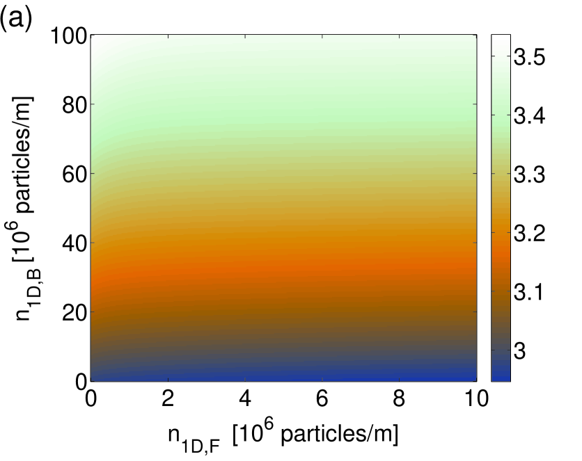
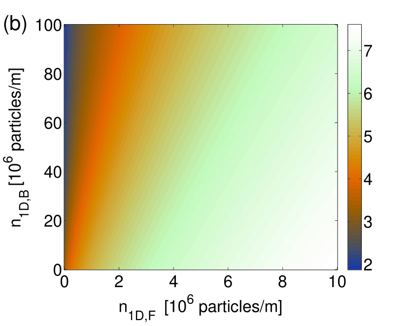
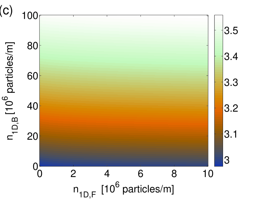
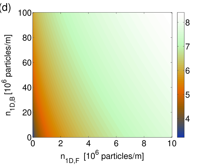
Figure 1: (Color online) Color-coded charts for the transverse widths of the bosonic and fermionic species, $\sigma_{\mathrm{B}}$ and $\sigma_{\mathrm{F}}$ (measured in units of ${\rm\mu}m$), as functions of the bosonic and fermionic 1D densities, $n_{1\mathrm{D,B/F}}$. (a) $\sigma_{\mathrm{B}}$ and (b) $\sigma_{F}$ for $a_{\mathrm{BF}}=-25$ nm. (c) $\sigma_{\mathrm{B}}$ and (d) $\sigma_{\mathrm{F}}$ for $a_{\mathrm{BF}}=25$ nm. The other parameters are $a_{\mathrm{B/F}}=5$ nm and $\omega_{t,\mathrm{B/F}}=1000$ Hz. Only fully polarized fermions are considered here.

The above results can be explained by the dependence of the interaction between the species on their densities. To do this, we define a single scattering parameter,

$${g_{e,\mathrm{B}}}={g_{\mathrm{B}}}\left[{1+2\frac{{{g_{\mathrm{BF}}}}}{{{g_{\mathrm{B}}}}}\frac{{{n_{1\mathrm{D},\mathrm{F}}}}}{{{n_{1\mathrm{D},B}}}}{{\left({1+{{\left({\frac{{{\sigma_{\mathrm{F}}}}}{{{\sigma_{\mathrm{B}}}}}}\right)}^{2}}}\right)}^{-1}}}\right],$$ (19)

and its counterpart for the fermions, obtained by replacing subscript $\mathrm{B}$ with $\mathrm{F}$. Making use of the so defined interaction parameter 19, in Eqs. 15 and 16, these equations assume the form given by

$$i\hbar{\partial_{t}}{f_{\rm{B}}}=\left[{-\frac{{{\hbar^{2}}}}{{2{m_{\rm{B}}}}}\partial_{Z}^{2}+{V_{1{\rm{D}},{\rm{B}}}}+\frac{{{g_{{\rm{e}}{\rm{,B}}}}}}{{2\pi\sigma_{\rm{B}}^{2}}}{{\left|{{f_{\rm{B}}}}\right|}^{2}}+\frac{{{\hbar^{2}}}}{{2{m_{B}}\sigma_{\rm{B}}^{2}}}+\frac{1}{2}{m_{B}}\omega_{t,{\rm{B}}}^{2}\sigma_{\rm{B}}^{2}}\right]{f_{\rm{B}}},$$ (20)

and

$$i\frac{\hbar}{{{\lambda_{1}}}}{\partial_{t}}{f_{\rm{F}}} = \left[{-\frac{{{\hbar^{2}}}}{{2{\lambda_{2}}{m_{\rm{F}}}}}\partial_{Z}^{2}+{V_{1D,{\rm{F}}}}+\frac{{{g_{{\rm{e}}{\rm{,F}}}}}}{{2\pi\sigma_{\rm{F}}^{2}}}{{\left|{{f_{\rm{F}}}}\right|}^{2}}+\frac{{{\hbar^{2}}}}{{2{m_{\rm{F}}}{\lambda_{2}}\sigma_{\rm{F}}^{2}}}+\frac{1}{2}{m_{\rm{F}}}\omega_{t,{\rm{F}}}^{2}\sigma_{\rm{F}}^{2}}\right.$$ (21)

$$+\left.{\frac{{{\hbar^{2}}\xi}}{{2{m_{\rm{F}}}}}\frac{{{C_{{\rm{F}},1{\rm{D}}}}}}{{\sigma_{\rm{F}}^{4/3}}}{{\left|{{f_{\rm{F}}}}\right|}^{4/3}}}\right]{f_{\rm{F}}}.$$

where the Eqs. 20 and 21 represented the motion equations for bosons and fermions separately, with effective scattering parameter $g_{\rm{e,B}}$ and $g_{\rm{e,F}}$ respectively. Figure 2 shows the variation of the effective scattering parameters, $g_{e,\mathrm{B}}$ and $g_{e,\mathrm{F}}$, with the inter-species scattering length, $a_{\mathrm{BF}}$. Figure 2(a) shows that the interaction between the bosons is suppressed when the interaction is attractive, and increases when it is repulsive. When the fermionic density is much lower that the bosonic density (circles), the influence of the variation of the interaction between the species on the effective interaction strength is minimal. Figure 2(b) shows the variation of the effective scattering parameter of the fermions ($g_{e,\mathrm{F}}$) under the same conditions as in Fig. 2(a), demonstrating the strong influence of the inter-species interaction on the fermions, due to the higher bosonic density. It is worthy to note that, for the range of $a_{\mathrm{BF}}$ presented in Fig. 2(b), $g_{e,\mathrm{F}}$ is about three orders of magnitude higher than $g_{\mathrm{F}}$. The inset in Fig. 2(b) additionally shows the dependence of $g_{e,\mathrm{F}}$ on the fermionic density $n_{1\mathrm{D},\mathrm{F}}$ (keeping $n_{1\mathrm{D},\mathrm{B}}$ fixed). A much larger number of bosons than that of fermions (the situation that that we address in this work), in the case of an attractive mixture, implies that the fermionic profile will be close to that of the bosonic gas. Accordingly, the Gaussian ansatz is appropriate for in both species, which is confirmed below by the comparison between 3D numerical and variational solutions.

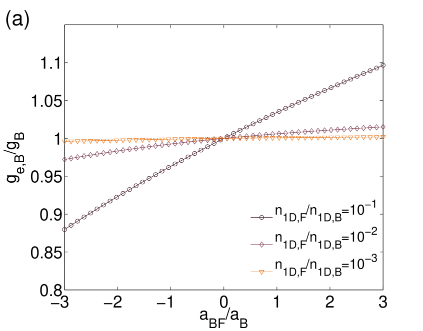
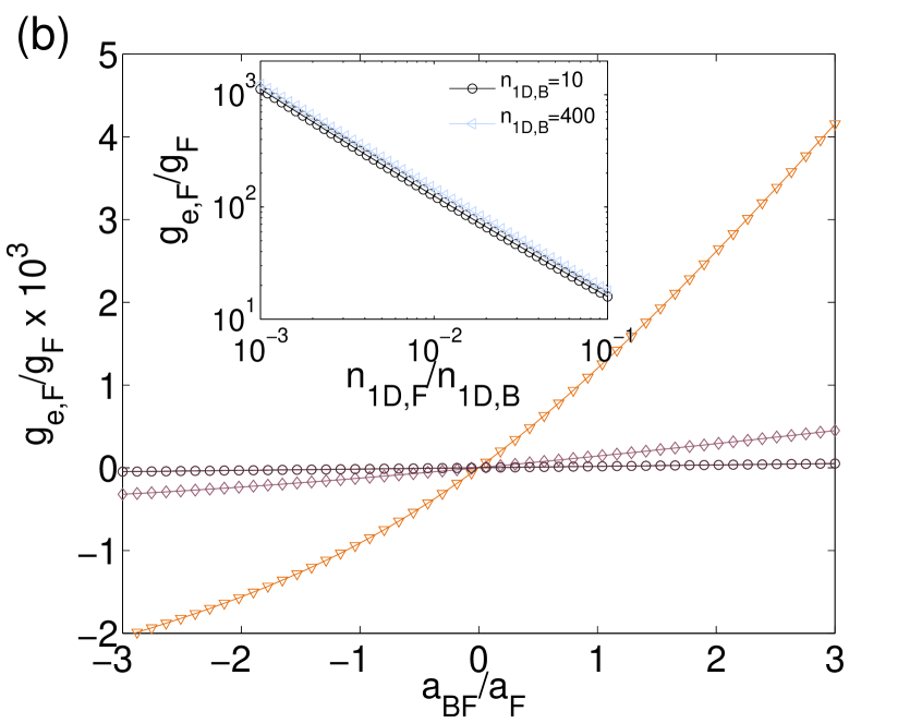
Figure 2: (Color online) The variation of the effective scattering parameters: (a) $g_{e,\mathrm{B}}/g_{\mathrm{B}}$ and (b) $g_{e,\mathrm{F}}/g_{\mathrm{F}}$ as a function of the interspecies scattering length $a_{\mathrm{BF}}/a_{\mathrm{B}}$ for three values of $n_{1\mathrm{D,F}}/n_{1\mathrm{D,B}}$. The parameters are $\omega_{t,\mathrm{B/F}}=1000$ Hz, $a_{\mathrm{B/F}}=5$ nm and $n_{1\mathrm{D},\mathrm{B}}=100$. The inset of the figure corresponds to $g_{\mathrm{BF}}/g_{\mathrm{B/F}}=1$ for two values of $n_{1\mathrm{D,B}}$.

2.2 The two-dimensional variational system

To derive 2D equations for the disc-shaped gas, the shape of the confinement potential is taken as (cf. Eq. (7) for the cigar-shaped configuration):

$${V_{\mathrm{B}/\mathrm{F}}}\left({\mathbf{r}}\right)={V_{2\mathrm{D},\mathrm{B}/\mathrm{F}}}\left({x,y}\right)+\frac{1}{2}{m_{\mathrm{B}/\mathrm{F}}}\omega_{z,\mathrm{B}/\mathrm{F}}^{2}{z^{2}},$$ (22)

where the second term corresponds to the strong harmonic trap acting along the $z$ direction. The corresponding factorized ansatz is adopted as ${\Psi_{\mathrm{B}/\mathrm{F}}}={\phi_{\mathrm{B}/\mathrm{F}}}\left({x,y}\right){u_{\mathrm{B}/\mathrm{F}}}\left({z;\xi_{\mathrm{B}/\mathrm{F}}\left({x,y,t}\right)}\right)$, where $u_{\mathrm{B}/\mathrm{F}}$ and $\phi_{\mathrm{B}/\mathrm{F}}$ are normalized to $1$ and $N_{\mathrm{B}/\mathrm{F}}$, respectively, and $u_{\mathrm{B}/\mathrm{F}}$ is represented by the Gaussian wave function,

$${u_{\mathrm{B}/\mathrm{F}}}\left({z;{\xi_{\mathrm{B}/\mathrm{F}}}}\right)=\frac{1}{{{\pi^{1/4}}\xi_{\mathrm{B}/\mathrm{F}}^{1/2}}}{\exp}\left(-\frac{{{z^{2}}}}{{2\xi_{\mathrm{B}/\mathrm{F}}^{2}}}\right),$$ (23)

${\xi_{\mathrm{B}/\mathrm{F}}}\left({x,y,t}\right)$ being the widths of the gas in the confined direction. Substituting the factorized ansatz (23) into action (1) and integrating over $z$, we arrive at the following expression for the effective 2D action:

$$\mathcal{S}=\int{dtdxdy\left(\mathcal{L}_{2D\mathrm{,B}}+\mathcal{L}_{2\mathrm{D},\mathrm{F}}+\mathcal{L}_{2\mathrm{D,BF}}\right)},$$ (24)

$$\mathcal{L}_{2\mathrm{D,B}}=i\frac{\hbar}{2}\left({\phi_{\mathrm{B}}^{\ast}{\partial_{t}}{\phi_{\mathrm{B}B}}-{\phi_{\mathrm{B}}}{\partial_{t}}\phi_{\mathrm{B}}^{\ast}}\right)-{V_{2D\mathrm{,B}}}{n_{2\mathrm{D,B}}}-{e_{2\mathrm{D,B}}},$$ (25)

$${\mathcal{L}_{2\mathrm{D},\mathrm{F}}}=i\frac{\hbar}{{2{\lambda_{1}}}}\left({\phi_{\mathrm{F}}^{\ast}{\partial_{t}}{\phi_{\mathrm{F}}}-{\phi_{\mathrm{F}}}{\partial_{t}}\phi_{\mathrm{F}}^{\ast}}\right)-{V_{2\mathrm{D},\mathrm{F}}}{n_{2\mathrm{D},\mathrm{F}}}-{e_{2\mathrm{D},\mathrm{F}}},$$ (26)

$${\mathcal{L}_{2\mathrm{D,BF}}}=-\frac{1}{{{\pi^{1/2}}}}\frac{{{g_{B\mathrm{F}}}}}{\sqrt{\xi_{\mathrm{B}}^{2}+\xi_{\mathrm{F}}^{2}}}{n_{2\mathrm{D},\mathrm{B}}}{n_{2\mathrm{D},\mathrm{F}}},$$ (27)

where $n_{2\mathrm{D,B/F}}\equiv\left|{\phi_{\mathrm{B}/\mathrm{F}}}\left({x,y}\right)\right|^{2}$ are the 2D particle densities of the boson and fermion species, and ${e_{2\mathrm{D,B}}}$ and ${e_{2\mathrm{D},\mathrm{F}}}$ are their energy densities:

$${e_{2\mathrm{D,B}}}=\frac{{{\hbar^{2}}}}{{2{m_{\mathrm{B}}}}}{\left|{{\nabla_{\bot}}{\phi_{\mathrm{B}}}}\right|^{2}}+\left[{\frac{{{g_{\mathrm{B}}}}}{{{\sqrt{8\pi}}{\xi_{\mathrm{B}}}}}{n}_{2\mathrm{D,B}}+\frac{{{\hbar^{2}}}}{{4{m_{\mathrm{B}}}\xi_{\mathrm{B}}^{2}}}}\right.+\left.{\frac{1}{4}{m_{\mathrm{B}}}\omega_{z,\mathrm{B}}^{2}\xi_{\mathrm{B}}^{2}}\right]{n_{2\mathrm{D},\mathrm{B}}},$$ (28)

$${e_{2\mathrm{D},\mathrm{F}}} = \frac{{{\hbar^{2}}}}{{2{\lambda_{2}}{m_{\mathrm{F}}}}}{\left|{{\nabla_{\bot}}{\phi_{\mathrm{F}}}}\right|^{2}}+\left[{\frac{{{g_{\mathrm{F}}}}}{{{\sqrt{8\pi}}{\xi_{\mathrm{F}}}}}{n_{2\mathrm{D},\mathrm{F}}}+\frac{{{\hbar^{2}}}}{{4\lambda_{2}{m_{\mathrm{F}}}\xi_{\mathrm{F}}^{2}}}+\frac{1}{4}{m_{\mathrm{F}}}\omega_{z,\mathrm{F}}^{2}\xi_{\mathrm{F}}^{2}}\right.$$ (29)

$$+\left.{\frac{{{\hbar^{2}}}}{{2{m_{\mathrm{F}}}}}\xi\frac{3}{{5\xi_{\mathrm{F}}^{2/3}}}{C_{2\mathrm{D},\mathrm{F}}}n_{2\mathrm{D},\mathrm{F}}^{2/3}}\right]{n_{2\mathrm{D},\mathrm{F}}},$$

with $C_{2\mathrm{D},\mathrm{F}}\equiv{(3/5)^{1/2}}{(6/(2s_{\mathrm{F}}+1))^{2/3}}\pi$ in Eq. (29).

The motion equations of the 2D system are obtained by the variation of the action $S$ given by Eq. (24) with respect to variables $\phi_{\mathrm{B}}$ and $\phi_{\mathrm{F}}$:

$$i\hbar{\partial_{t}}{\phi_{\mathrm{B}}} = \left[{-\frac{{{\hbar^{2}}}}{{2{m_{B}}}}\nabla_{\bot}^{2}+{V_{2\mathrm{D,B}}}+\frac{1}{{{\pi^{1/2}}}}\frac{{{g_{\mathrm{BF}}}}}{\sqrt{\xi_{\mathrm{B}}^{2}+\xi_{\mathrm{F}}^{2}}}{n_{2\mathrm{D},\mathrm{F}}}}+\frac{{{g_{\mathrm{B}}}}}{{\sqrt{2\pi}{\xi_{\mathrm{B}}}}}{{\left|{{\phi_{\mathrm{B}}}}\right|}^{2}}\right.$$ (30)

$$+\left.\frac{{{\hbar^{2}}}}{{4{m_{\mathrm{B}}}\xi_{\mathrm{B}}^{2}}}+\frac{1}{4}{m_{\mathrm{B}B}}\omega_{z,\mathrm{B}}^{2}\xi_{\mathrm{B}}^{2}\right]{\phi_{\mathrm{B}},}$$

$$i\frac{\hbar}{{{\lambda_{1}}}}{\partial_{t}}{\phi_{\mathrm{F}}} = \left[{-\frac{{{\hbar^{2}}}}{{2{\lambda_{2}}{m_{\mathrm{F}}}}}\nabla_{\bot}^{2}+{V_{2D,\mathrm{F}}}+\frac{1}{{{\pi^{1/2}}}}\frac{{{g_{\mathrm{BF}}}}}{\sqrt{\xi_{\mathrm{B}}^{2}+\xi_{\mathrm{F}}^{2}}}{n_{2\mathrm{D,B}}}}+\frac{{{g_{\mathrm{F}}}}}{{\sqrt{2\pi}{\xi_{\mathrm{F}}}}}{\left|{{\phi_{\mathrm{F}}}}\right|^{2}}\right.$$ (31)

$$+\left.\frac{{{\hbar^{2}}}}{{2{m_{\mathrm{F}}}}}\xi\frac{1}{{\xi_{\mathrm{F}}^{2/3}}}{C_{2\mathrm{D},\mathrm{F}}}{\left|{{\phi_{\mathrm{F}}}}\right|^{4/3}}+{\frac{{{\hbar^{2}}}}{{4\lambda_{2}{m_{\mathrm{F}}}\xi_{\mathrm{F}}^{2}}}+\frac{1}{4}{m_{\mathrm{F}}}\omega_{z,\mathrm{F}}^{2}\xi_{\mathrm{F}}^{2}}\right]{\phi_{\mathrm{F}}.}$$

Relations between $\xi_{\mathrm{B}/\mathrm{F}}$ and $\phi_{\mathrm{B}/\mathrm{F}}$ are produced by the Euler-Lagrange equations associated to $\xi_{\mathrm{B}/\mathrm{F}}$:

$${\kappa_{I,B}}\xi_{\mathrm{B}}^{4}-\frac{{{g_{B}}}}{\sqrt{2\pi}}{n_{2\mathrm{D,B}}}{\xi_{\mathrm{B}}}-\frac{{{\hbar^{2}}}}{{{m_{\mathrm{B}}}}}=0,$$ (32)

$${\kappa_{I,\mathrm{F}}}\xi_{\mathrm{F}}^{4}-\frac{{2{\hbar^{2}}}}{{5{m_{\mathrm{F}}}}}\xi{C_{2\mathrm{D},\mathrm{F}}}n_{2\mathrm{D},\mathrm{F}}^{2/3}\xi_{\mathrm{F}}^{4/3}-\frac{g_{\mathrm{F}}}{\sqrt{2\pi}}{n_{2\mathrm{D},\mathrm{F}}}{\xi_{\mathrm{F}}}-\frac{{{\hbar^{2}}}}{\lambda_{2}m_{\mathrm{F}}}=0$$ (33)

where ${\kappa_{I,\mathrm{F}}}\equiv{m_{\mathrm{F}}}\omega_{z,\mathrm{F}}^{2}+2{g_{\mathrm{BF}}}{n_{2\mathrm{D,B}}}/[{{\pi^{1/2}}{{({\xi_{\mathrm{B}}^{2}+\xi_{\mathrm{F}}^{2}})}^{3/2}}}]$. Equations (32) and (33) for $\xi_{\mathrm{B}/\mathrm{F}}$ were solved numerically. The four graphs in Fig. 3 show the dependence of $\xi_{\mathrm{B}}$ and $\xi_{\mathrm{F}}$ (in the left and right columns, respectively) on $n_{2\mathrm{D,B/F}}$, for the attractive and repulsive mixtures (top and bottom panels, respectively). The analysis for the attractive case can be divided into two parts: when the boson density is high, the fermions gas tends to compress, so that at low densities its width is found to be even less than that of the boson gas, a situation that tends to reverse for high fermionic densities; for low bosonic densities, the width of the boson gas rapidly decreases with the increase of the fermionic density, until becoming nearly constant, while, on the contrary, the width of the fermion gas increases progressively when its density is higher. Conversely, when the mixture is repulsive, the situation is similar to that outlined above for the 1D setting: low densities of the mixtures cause the gas to compress, while high densities cause the mixture to expand, this trend being much stronger for the fermion component.

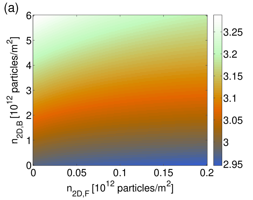
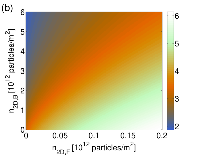
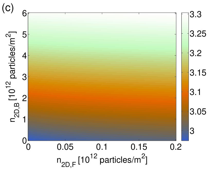
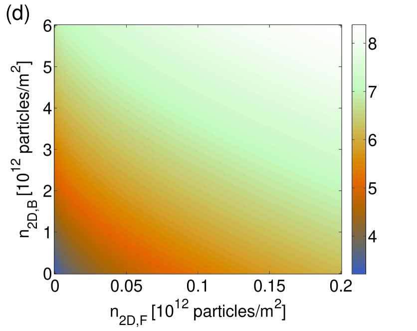
Figure 3: (Color online) Color-coded charts for the transverse widths of the bosonic and fermionic species, $\xi_{\mathrm{B}}$ and $\xi_{\mathrm{F}}$ (measured in units of ${\rm\mu}m$), as functions of the bosonic and fermionic 2D densities, $n_{2\mathrm{D,B/F}}$. (a) $\xi_{\mathrm{B}}$ and (b) $\xi_{\mathrm{F}}$ for $a_{\mathrm{BF}}=-25$ nm. (c) $\xi_{\mathrm{B}}$ and (d) $\xi_{\mathrm{F}}$ for $a_{\mathrm{BF}}=25$ nm. The other parameters are $a_{\mathrm{B/F}}=5$ nm and $\omega_{z,\mathrm{B/F}}=1000$ Hz. Only fully polarized fermions are considered here.

To determine the influence that one species exerts on the other in 2D, we define the effective scattering parameters, cf. a similar definition (19) adopted in the 1D case:

$${g_{e,\mathrm{B}}}={g_{\mathrm{B}}}\left[1+\sqrt{2}\frac{g_{\mathrm{BF}}}{g_{\mathrm{B}}}\frac{n_{2\mathrm{D},\mathrm{F}}}{n_{2\mathrm{D},B}}\left(1+\left(\frac{\xi_{\mathrm{F}}}{\xi_{\mathrm{B}}}\right)^{2}\right)^{-1/2}\right],$$ (34)

$g_{e,\mathrm{F}}$ being produced by replacing subscript $\mathrm{B}$ with $\mathrm{F}$. As shown in detail below, our calculations were performed assuming the same order of magnitude for the number of particles for both 1D and 2D cases (for this reason that the effective 1D density is about $10$ times the magnitude of its 2D counterpart). With regard to this, conclusions concerning the effective interaction strength, which follow in the 1D setting from Fig. 2, apply to 2D case as well.

3 Numerical Results

Our analysis was developed for the GS and dynamics of perturbations around it in the presence of the 3D harmonic-oscillator trap of the following form:

$${V_{\mathrm{B/F}}}\left({\mathbf{r}}\right)=\frac{1}{2}{m_{\mathrm{B/F}}}\left({\omega_{x,\mathrm{B/F}}^{2}{x^{2}}+\omega_{y,\mathrm{B/F}}^{2}{y^{2}}+\omega_{z,\mathrm{B/F}}^{2}{z^{2}}}\right),$$ (35)

In particular, for the GS of the 1D and 2D settings we focused on determining the spatial correlation $C_{s}$ between the spatial particle densities in both species, defined as

$${C_{s}}\left({{\bar{n}_{B}},{\bar{n}_{\mathrm{F}}}}\right)=\frac{{\left\langle{{\bar{n}_{B}}{\bar{n}_{\mathrm{F}}}}\right\rangle}}{\sqrt{\left\langle{\bar{n}_{B}^{2}}\right\rangle\left\langle{\bar{n}_{\mathrm{F}}^{2}}\right\rangle}},$$ (36)

where ${{\bar{n}}_{\mathrm{B}/\mathrm{F}}}={n_{\mathrm{B}/\mathrm{F}}}-\left\langle{{n_{\mathrm{B}/\mathrm{F}}}}\right\rangle$, $\left\langle{}\right\rangle$ standing for the spatial average. For dynamical perturbations around the GS, a spatiotemporal correlation, which is defined by replacing the spatial average with the spatiotemporal average, is known as the Pearson coefficient $C_{s-t}$ [54]. The GSs in the 1D and 2D cases were found by means of the imaginary-time integrations of Eqs. (15), (16) and (30), (31), respectively.

3.1 Results in one dimension.

3.1.1 Accuracy of the variational method as a function of scattering parameter $a_{\mathrm{BF}}$ for the ground states.

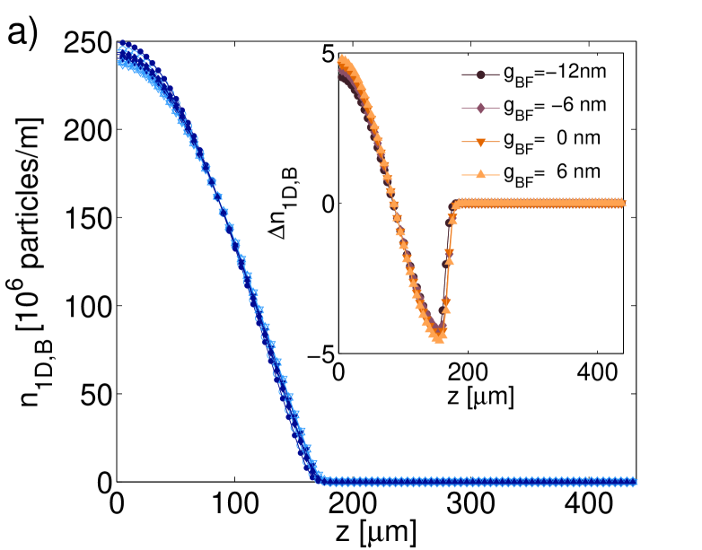
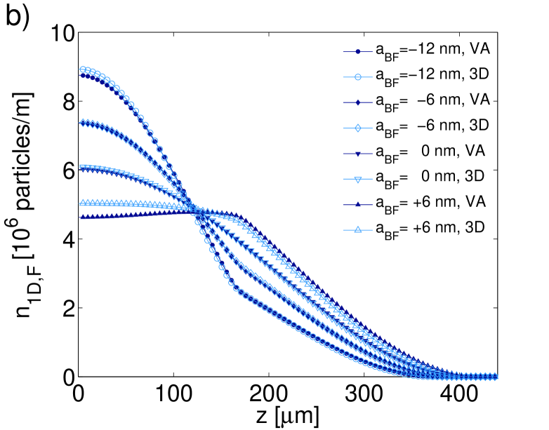
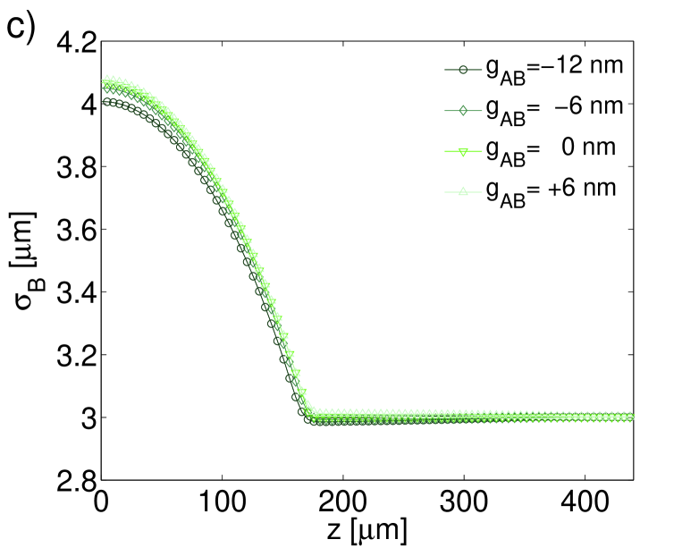
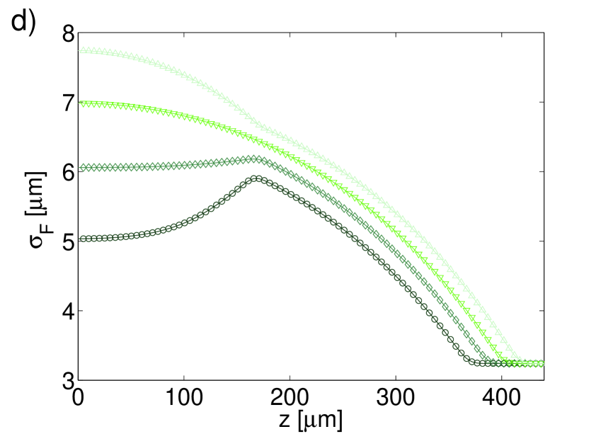
Figure 4: (Color online) Profiles of the particle density (as produced by the VA and 3D calculations, see inset in panel (b)), and the width in the confined direction, for the bosonic and fermionic components, for five values of $a_{\mathrm{BF}}$, as defined in the panels. (a) $n_{1\mathrm{D,B}}$, (b) $n_{1\mathrm{D,F}}$, (c) $\sigma_{\mathrm{B}}$, and (d) $\sigma_{\mathrm{F}}$. The parameters are $N_{\mathrm{B}}=5\times 10^{4}$, $N_{\mathrm{F}}=2.5\times 10^{3}$, $a_{\mathrm{B/F}}=5$ nm, $\omega_{z,\mathrm{B/F}}=30$ Hz and $\omega_{t,\mathrm{B/F}}=1000$ Hz. The inset in (a) shows the difference between both methods, VA and 3D, by means of $\Delta n_{\mathrm{1D,B}}=\rho_{\mathrm{1D,B}}-n_{\mathrm{1D,B}}$.

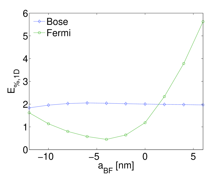
Figure 5: (Color online) One-dimension overall percentage error for both species (see the definition in the text). The parameters are the same as in Fig. 4

As a starting point in the 1D case with free coordinate $z$, we analyze the effect of the magnitude and sign of the interaction parameter on the spatial profile of both species, and the accuracy of the variational method (see Eqs. 15 - 18) compared to the 3D solution, by varying the scattering length $a_{\mathrm{D,B}}$. The plots in Fig. 4 shows this situation, with panels 4(a) and  4(b) corresponding to the profiles of $n_{1\mathrm{D,B}}$ and $n_{1\mathrm{D},\mathrm{F}}$, respectively, where the inset in panel 4(b) specifies whether the profile was produced by the VA or by means of the 3D solution, while 4(c) and  4(d) correspond to the profiles of $\sigma_{\mathrm{B}}$ and $\sigma_{\mathrm{F}}$. The mixture with many more bosons than fermions is considered here: $N_{\mathrm{B}}=5\times 10^{4}$, $N_{\mathrm{F}}=2.5\times 10^{3}$. Because of this condition, the bosonic profile is mainly determined by its self-interaction and the external potential. First, we deal with the influence of the interspecies interaction ($g_{\mathrm{BF}}$) on the density profile, and then address an error resulting from the variational approach. Figure 4(a) shows that variations of the bosonic density profile are very small in comparison to the significant changes of the inter-species scattering length. The situation is opposite for the fermionic species. As the repulsive scattering length increases, the fermions tend to be pushed to the periphery of the bosonic-gas density profile. This phenomenon is known as demixing [27, 32, 35, 52]. On the other hand, for the attractive case, fermions are, naturally, concentrated in the same region where the bosons are located. Figures Fig. 4(c) and 4(d) show that the width of the bosonic profile (Fig. 4(c)) slightly increases as going from the inter-species attraction to repulsion. A similar trend is observed for fermions, see Fig. 4(d), but amplified in the spatial zone of the interaction with the bosons, where the gas is compressed in the case of the attraction and expands in the case of the repulsion. It is noted that the fermionic component expands in the confined direction much more than its bosonic counterpart, and that the fermionic width fluctuates markedly with changes in density. Now, to analyze the accuracy of the method we solved Eqs. 5 and 6 and obtained the 1D density associated through of $\rho_{1D,\mathrm{B/F}}=\int\int\left|\Psi_{\mathrm{B/F}}\right|^{2}dxdy$. The inset in panel 4(a) shows that the difference between the bosonic profiles obtained by both methods (VA or 3D) is $\sim 2\%$ of the maximum density for all cases (the fact that the error changes very little with variations in $a_{\mathrm{BF}}$ is a consequence of the greater number of bosons). Figure 4(b) shows that, for the case of the attractive mixture, the variational profile is very close to the 3D result, in particular for the case of $a_{\mathrm{BF}}=-6nm$. For the repulsive mixture, it is observed that the error increases, which is a consequence of the lower fermionic density at the center of the 3D harmonic potential, dominated for the bosons, hence a monotonously decreasing function in the transverse direction, such as the Gaussian, is not a sufficiently good approximation. We define the global error for the variational method as $E_{\%,\mathrm{1D}}=\int\left|\rho_{\mathrm{1D}}-n_{\mathrm{1D}}\right|dz$ (for both species). Figure 5 shows the global error for both species as a function of the scattering parameter, $a_{\mathrm{BF}}$. This picture demonstrates that the error for the bosonic species is around $2\%$, and it does not change much (as already noted in the comment to Fig. 4(a)). For the fermions, the error attains a minimum value $\sim 0.5\%$ at $a_{\mathrm{BF}}\approx 4$nm, thus corroborating that the Gaussian is a very good approximation. This is a consequence of the fact that, for this value of $a_{\mathrm{BF}}$, the interspecies interaction term practically compensates the Pauli repulsion term, making the dynamics of the fully polarized Fermi gas close to that giverned by the Schödinger equation (recall that the Gaussian is the solution for the ground state). When the mixture becomes more attractive, the fermionic dynamics is dominated by the bosons, producing a similar error for both species, while for the repulsive mixture the Gaussian approximation is not appropriate. Interestingly, for the non-interacting mixture, the error for the fermions is smaller than for the bosons, because the fermionic density is very low, making the self-interaction terms weak in comparison to the external potential, therefore it is appropriate to use the Gaussian ansatz for describing the 1D dynamics. Using the TF profile may produce, in principle, better results, but the respective analysis would be cumbersome.

3.1.2 Spatial correlations in the ground state.

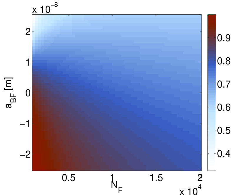
Figure 6: (Color online) The color-coded plot of the spatial correlation $C_{s}$, defined as per Eq. (36), as a function of the fermionic number, $N_{\mathrm{F}}$, and the scattering length of the inter-species interaction, $a_{\mathrm{BF}}$. Other parameters are $N_{\mathrm{B}}=5\times 10^{4}$, $a_{\mathrm{B/F}}=5$ nm, $\omega_{z,\mathrm{B/F}}=30$ Hz and $\omega_{t,\mathrm{B/F}}=1000$ Hz.

As the first application, we calculate the spatial correlation between densities of the two species ($C_{s}$), as defined by Eq. (36) for a wide range of parameters, ranging from very attractive to to very repulsive mixtures. We keep in mind that the variational calculation produces a minor error for attractive mixtures, therefore the values obtained for the repulsive case will be considered as help to asses the validity of our analysis. The eventual objective is to produce a parameter which determines the mutual influence of both species. In the Fig. 6, the spatial correlation $C_{s}$ is shown versus $N_{\mathrm{F}}$ and $a_{\mathrm{BF}}$ , which shows that, for an attractive interaction, $C_{s}$ reaches values greater than $0.8$ (in the mixed state), whereas for the repulsive interaction $C_{s}$ decreases until reaching values around $C_{s}=0.3$ (in the demixed state). It is also noted that the number of fermions strongly affects the dependence of the correlation on the inter-species scattering length. When $N_{\mathrm{F}}$ increases, the difference between the maximum and the minimum value of $C_{s}$ decreases, as $a_{\mathrm{BF}}$ varies from $-25$ nm to $+25$ nm, tending to reach values close to $C_{s}=0.8$, which is the value attained in the absence of the interaction, depending only on the presence of the same trap acting on both components.

3.1.3 Dynamics near the ground state

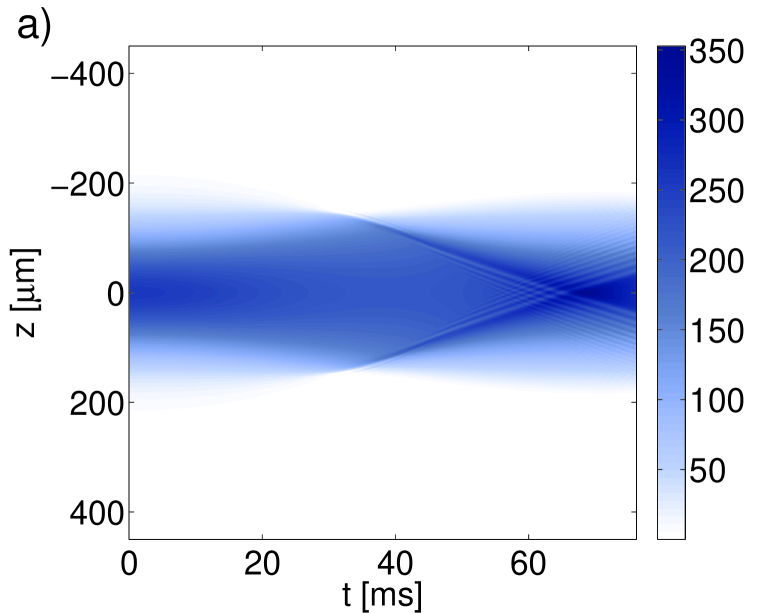
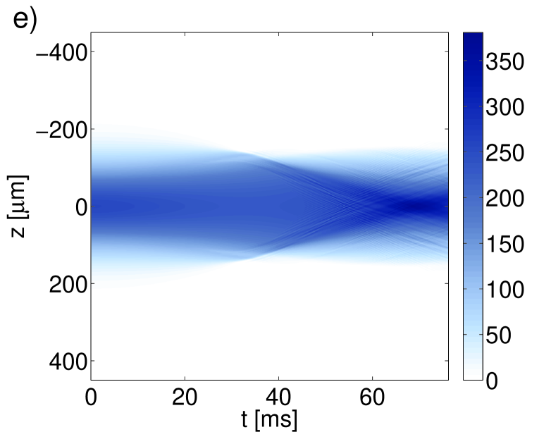
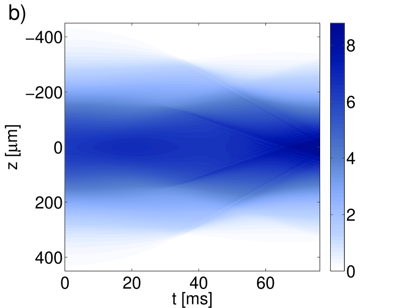
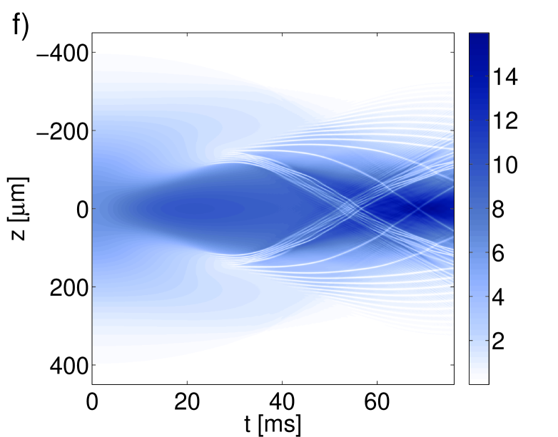
Figure 7: (Color online) Space-time diagrams for the conservative dynamics of bosons (above) and fermions (bottom), for three different values of the interspecies scattering parameter: (a)$-$(b) $a_{\mathrm{BF}}=-6nm$, (c)$-$(d) $a_{\mathrm{BF}}=-12nm$, and (e)$-$(f) $a_{\mathrm{BF}}=-14nm$. The initial conditions are the same in all cases and are described in the text. Other parameters are the same as in Fig. 4

We begin the study of conservative dynamics, considering a mixture with arbitrary initial conditions for the 1D fields: we assume a Gaussian shape along the $z$-axes with widths (standard deviation) of $100\mu$m and $200\mu$m for bosons and fermions, respectively. Figure 7 shows three cases of the temporal evolution with these initial conditions for $a_{\mathrm{BF}}=-6nm$, $a_{\mathrm{BF}}=-12nm$, and $a_{\mathrm{BF}}=-14nm$. In the first case (panels 7(a) and  7(b)), it is observed that the densities converge towards the center of the potential in an expected pattern of oscillations around the potential minimum; in addition, the fermions are affected by bosons, as can be seen for the mark left by the bosons in the fermionic density. For the second case (panels 7(c) and  7(d)), it is observed that the increase in the magnitude of the attractive interaction generates dark solitons in the fermionic density, some of which shows oscillatory dynamics very similar to that observed, experimentally and theoretically, in Refs. [55]-[60]. Finally, the last case (panels 7(e) and  7(f)) shows that further increase in the magnitude of the interspecies interaction generates a larger number of dark solitons. In other words, we show that the attractive interaction of fermions with bosons in a state different from the ground state eventually generates a gas of dark solitons.

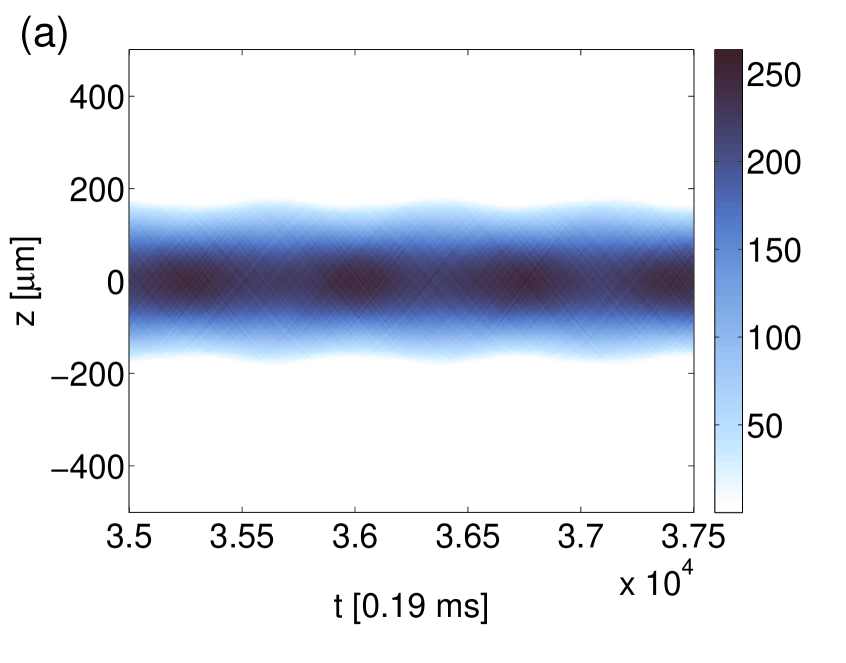
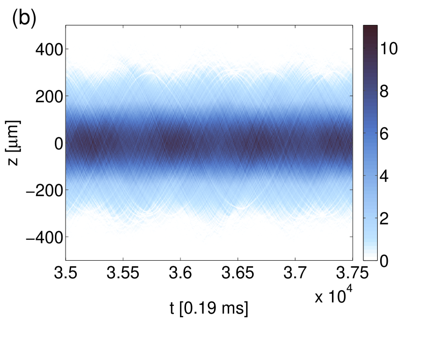
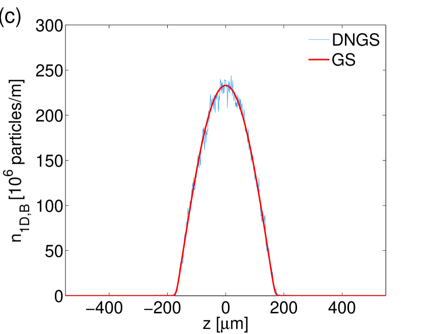
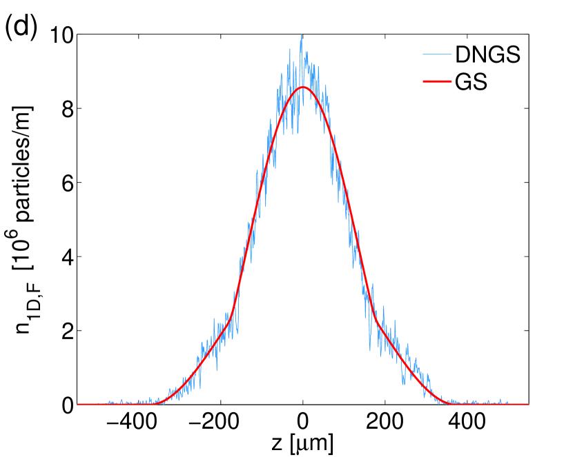
Figure 8: (Color online) (a) and (b) Spatiotemporal evolution of the bosonic and fermionic densities, respectively, in the case of suddenly switching the inter-species interaction in the 1D ground state which corresponded to $a_{\mathrm{BF}}=0$. (c) and (d) Bosonic and fermionic density profiles at the end of the simulations (the blue lines) compared to the ground state (red line), at the same values of physical parameters, which are $N_{\mathrm{B}}=5\times 10^{4}$, $N_{\mathrm{F}}=2.5\times 10^{3}$, $a_{\mathrm{B/F}}=5$ nm, $a_{\mathrm{BF}}=-15$ nm, $\omega_{z,\mathrm{B/F}}=30$ Hz, and $\omega_{t,\mathrm{B/F}}=1000$ Hz.

Now we aim to address the system’s dynamics in the vicinity of the GS. We start with the GS found in the absence of the inter-species interaction ($a_{\mathrm{BF}}=0$). Then, at $t=0$, we switch the interaction on, which may imply the application of the magnetic field, that gives rise to $a_{\mathrm{BF}}\neq 0$ via the FR. Figure  8 shows an example of the ensuing evolution in the attractive mixture with $a_{\mathrm{BF}}=-15$ nm, the fermionic component being fully polarized. Panels  8(a) and (b) display space-time diagrams of oscillations of the bosonic and fermionic densities in the dynamical state. Panels 8(c) and (d) compare the density profiles at the end of the simulations with the GS of the interacting mixture. It is seen that the dynamics amount to rapid fluctuations around the GS. Figure 7 makes it clear that the spatiotemporal dynamics of fermions in panel 8(b) does not reduce to noise around the ground state. It rather corresponds to a gas of dark solitons oscillating in the harmonic potential. Moreover, the fact that the spatiotemporal diagram has been produces for the time when the system is in the stationary regime suggests that the dark solitons are fully stable. Note that the noise observed in the bosonic component is clearly caused by the fermionic dark solitons.

Now, we measure how correlated the densities remain in time. Similar to what is observed in Fig. 6, Fig. 9 shows that the spatial-correlation parameter $C_{s}$, defined as per given Eq. (36) rapidly decreases following the transition from negative to positive values of $a_{\mathrm{BF}}$ (the mixing-demixing transition). When the inter-species interaction is more attractive, it increases the correlations, imposing spatiotemporal synchronization of density fluctuations. In the case of strong repulsion, $a_{\mathrm{BF}}=50$ nm, correlation fluctuations are suppressed because the system falls into a demixed state.

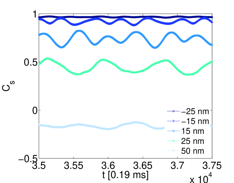
Figure 9: (Color online) The evolution of spatial correlation $C_{s}$ in the dynamical states near the ground state for five values of $a_{\mathrm{BF}}$, as indicated in the figure. The parameters are the same as in Fig. 8.

Figure 10 presents the analysis of the spatiotemporal synchronization of the mixture, where three possible regimes are considered for the fermions: fully polarized, BCS, and unitarity. Parameters of the the Lagrangian density for each fermionic regime are given in Table 1. The synchronization was calculated through the Person coefficient $C_{s-t}$ defined above. For each of the three cases, the spatial correlation, $Cs,$ was calculated too. When the interaction is attractive, there is no discrepancy between the synchronization and correlation curves. On the other hand, in all the three regimes it is observed that, as the interaction becomes more repulsive, the synchronization of the mixture decreases in comparison to the spatial correlation. This trend enhances as the system approaches the demixing transition. Another generic feature is that stronger correlations between the species near the GS imply a stronger synchronization on the spatiotemporal dynamics too.

The correlation properties are different for the distinct fermionic regimes. $C_{s-t}$ is always positive for the system with fully polarized fermions and in the BCS regime, decreasing as the interaction gets more repulsive. On the other hand, the unitarity regime features significant differences: at first, $C_{s-t}$ grows to a maximum value at $a_{\mathrm{BF}}=-10$ nm; then it decreases, reaching negative values of $C_{s-t}/C_{s}$ in the demixed state. In all the cases, no significant difference are observed between $C_{st}$ and $C_{s}$ in the case of the attractive Bose-Fermi interaction, i.e., a highly correlated GS supports the dynamical synchronization too.

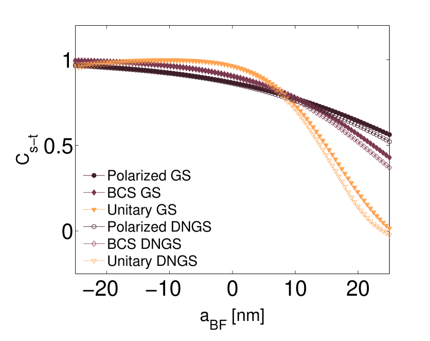
Figure 10: (Color online) Spatiotemporal correlation $C_{s-t}$ versus $a_{\mathrm{BF}}$ for the ground state (GS) and in the dynamics near the ground state (“DNGS”) for three fermions regimes: polarized, BCS, and unitarity. The parameters are $N_{\mathrm{B}}=5\times 10^{4}$, $N_{F}=2.5\times 10^{3}$, $a_{\mathrm{B/F}}=5$ nm, $\omega_{z,B/F}=30$ Hz and $\omega_{t,\mathrm{B/F}}=1000$ Hz. Table 1 provides parameters that correspond to the different regimens in the Lagrangian density.

3.1.4 Accuracy of the variational method for the spatiotemporal dynamics

In the Sec. 3.1.3 some examples of spatio-temporal dynamics were presented without discussing the accuracy of the results. In Fig. 11 the spatio-temporal dynamics of the 1D density is displayed as produced by the solution of the 3D equations 5 and  6, using the same procedure as in Section 3, for initial conditions similar to those used in Fig. 7 but with $a_{\mathrm{BF}}=-10nm$. The initial conditions for the 3D dynamics are given by the ansatz in Eq. 8, with the Gaussian profile along the $z$-axes, similar to those used in the Fig. 7. Panels 11(a) and  11(b) show spatio-temporal diagrams of the bosonic and fermionic density, respectively, making the emergence of dark solitons obvious, see also Fig. 7. This result corroborates that the dark solitons will emerge too in the 3D dynamics, which is approximated by the present 1D model. The other panels show a comparison of the 1D spatial profiles, as obtained from 3D simulations and the 1D VA, for three instants of time: $t=0ms$ (panels 11(c) and  11(d)), $t=25ms$ (panels 11(e) and  11(f)), and $t=50ms$ (panels 11(g) and  11(h)). The results demonstrate that the VA profiles are very similar to their counterparts produced by the 3D simulations, hence the present approximation provides good accuracy and allows one to study dynamical features of the Bose-Fermi mixture in a sufficiently simple form.

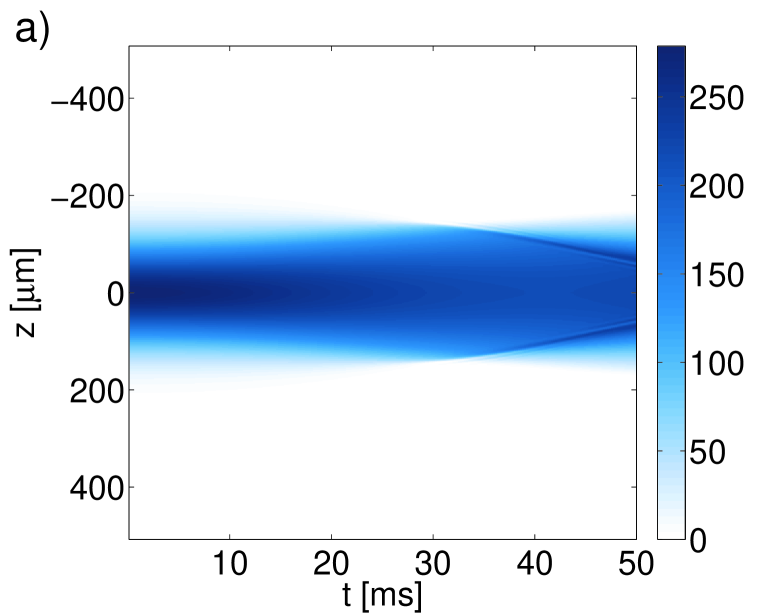
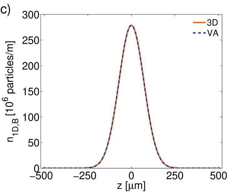
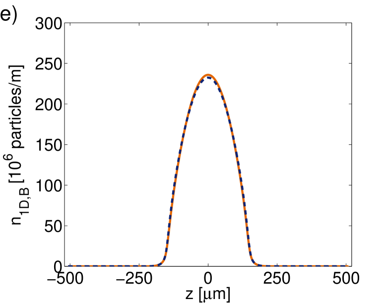
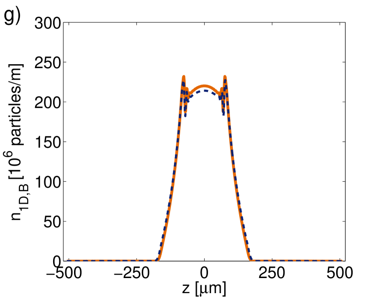
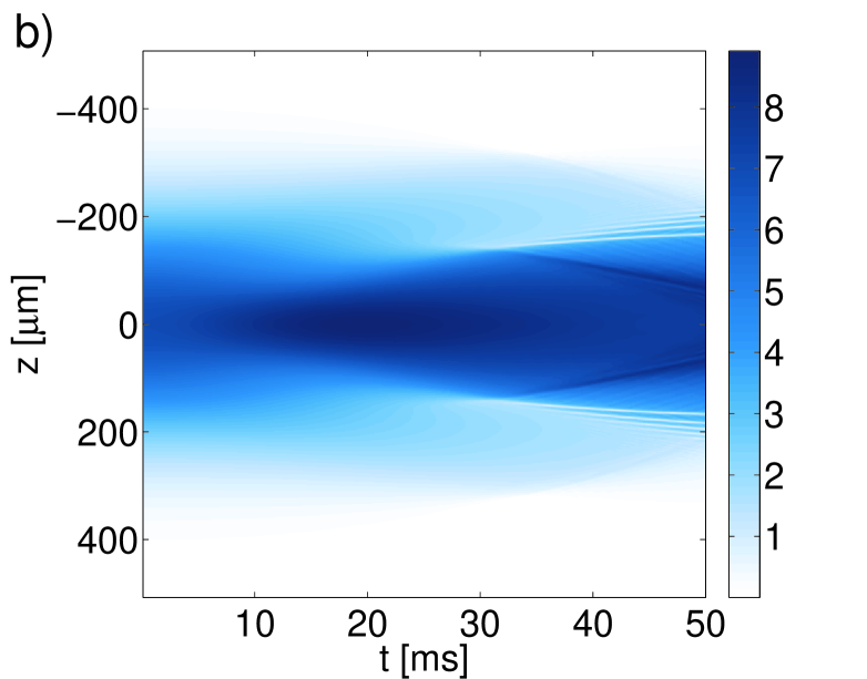
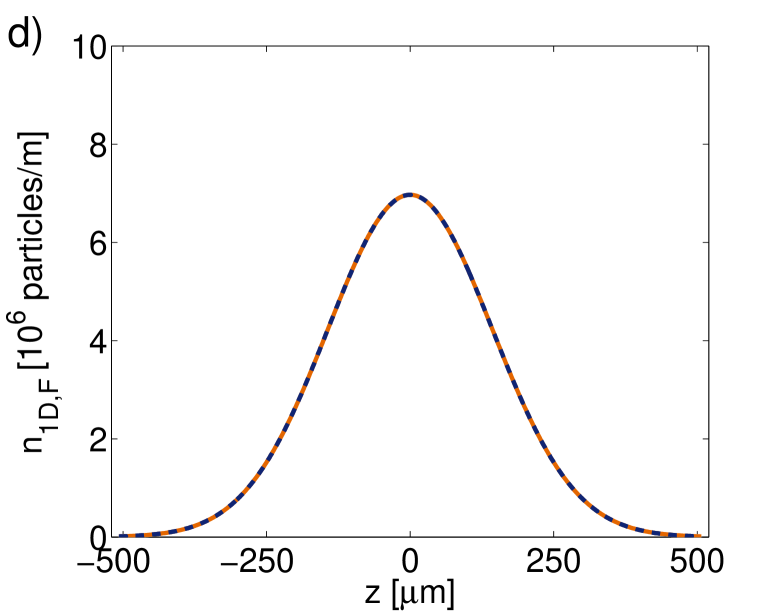
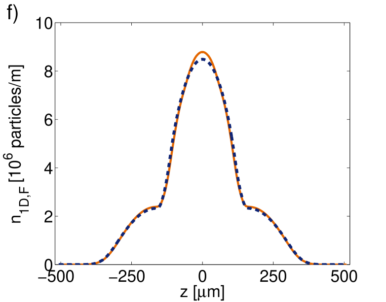
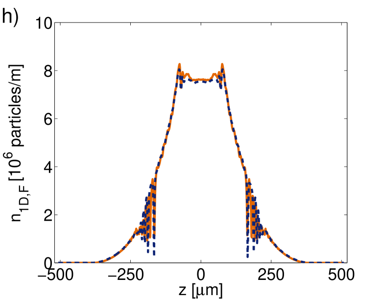
Figure 11: (Color online) Comparison of the dynamics, as obtained from the 1D variational approximation, and from the 3D simulations. Spatiotemporal diagrams for bosons (a) and fermions (b) are obtained from the 3D simulations. The other panels show spatial profiles for: (c)$-$(d) $t=0ms$, (e)$-$(f) $t=25ms$, and (e)$-$(f) $t=50ms$. Here $a_{\mathrm{BF}}=-10nm$, the initial conditions and other fixed parameters being the same as in Fig. 7.

3.2 Results in two dimensions.

3.2.1 Accuracy of the variational method as a function of scattering parameter $a_{\mathrm{BF}}$ for the ground state.

In the 2D setting, we studied the GS of the BFM, fixing the number of bosons to $N_{\mathrm{B}}=5\times 10^{4}$ (similar to the value used in the 1D case), which was and much greater than the number of fermions. Fig. 12 shows the profile of the 2D bosonic and fermionic densities, $n_{2\mathrm{D},\mathrm{B}/\mathrm{F}}$ (top), as obtained from the VA and 3D simulations, and the widths of the mixture in the transverse direction, $\xi_{\mathrm{B}/\mathrm{F}}$ (bottom), with respect to the radial coordinate. To obtain the 2D profile from the 3D simulations (results of solving Eqs. 5 and  6), we integrate the 3D density along the $z$ so that $\rho_{\mathrm{2D,B/F}}=\int\left|\Psi_{\mathrm{2D,B/F}}\right|dz$. The panels for the bosonic and fermionic components are displayed on the left and right, respectively. The results are very similar to what was observed in the 1D case in Fig. 4, for the same value of the physical parameters. Therefore, the following conclusions are also similar to what inferred in the 1D setting: the repulsive mixture concentrates the bosons at the center, while the attractive mixture concentrates both species at the center. Panels 12(c) and 12(d) show that only the width of the fermionic density profile varies significantly with the change of the scattering length of the inter-species interaction, which is consequence of a greater number of bosons than fermions. It is clearly seen that fermions are stronger confined when the interaction is attractive, and their spatial distribution significantly expands when the interaction is repulsive. Similar results have been observed in [27, 28, 32].

Now, to compare the results obtained from the VA with those produced by the 3D simulations, we note that both profiles are practically identical, except for the repulsive case in which a discrepancy is observed (smaller than in the 1D case). The inset in panel 12(a) shows that the difference between the two results has a magnitude of nearly three orders of magnitude lower than the density itself. The error is lower than in the 1D case because the 2D reduction is closer to the full 3D model.

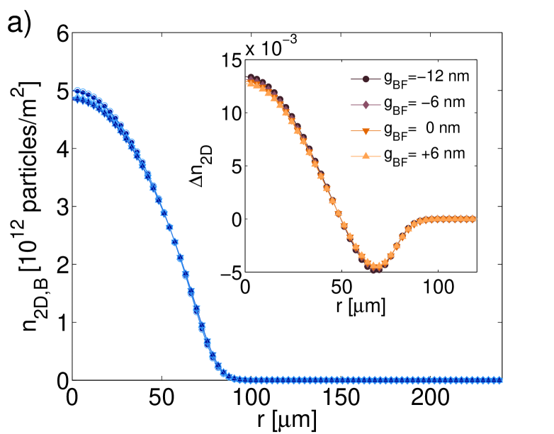
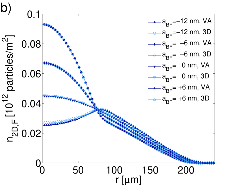
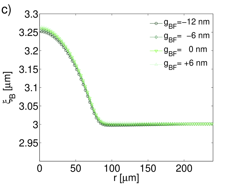
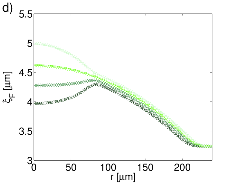
Figure 12: (Color online) The radial profile of the 2D particle density (for the VA and 3D simulations, see the inset in panel (b)), and the respective width in the transverse direction ($z$) of the bosonic and fermionic profiles, for five values of $a_{\mathrm{BF}}$ (see insets in the panels): (a) $n_{2\mathrm{D},\mathrm{B}}$, (b) $n_{2\mathrm{D,F}}$, (c) $\xi_{\mathrm{B}}$, and (d) $\xi_{\mathrm{F}}$. The parameters are $N_{\mathrm{B}}=5\times 10^{4}$, $N_{\mathrm{F}}=2.5\times 10^{3}$, $a_{\mathrm{B/F}}=5$ nm, $\omega_{z,\mathsf{B/F}}=1000$ Hz, and $\omega_{x,\mathrm{B/F}}=\omega_{y,\mathrm{B/F}}=30$ Hz. The inset in panel (a) shows the difference between both methods, VA and 3D, where $\Delta n_{\mathrm{2D}}\equiv\rho_{\mathrm{2D}}-n_{\mathrm{2D}}$.

Now, similar to the 1D case, we define the overall percentage error of the VA as $E_{\%,\mathrm{2D}}=\int\int\left|\rho_{\mathrm{2D}}-n_{\mathrm{2D}}\right|dxdy$ (for both species). Figure 13 shows the error for both species as a function of interspecies scattering parameter ($a_{\mathrm{BF}}$). For bosons it is around of $0.2\%$ (one order of magnitude lower than in the 1D case), and does not change much (as shown in the inset to Fig. 12(a)). For fermions the error is greater than for bosons throughout the observed range, but it is quite small for the attractive mixture. Like in the 1D case, the error increases for the repulsive mixture, but remains lower than that calculated for bosons in the 1D case. In summary, the 2D approximation is very accurate, implying, as shown below, that the description of the dynamics is also more accurate in this case.

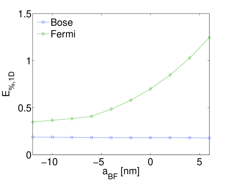
Figure 13: (Color online) 2D overall percentage error for both species (the definition is given in the text). Parameters are the same as in Fig. 12.

3.2.2 Spatial correlations of the two-dimensional density

Here we again apply the formalism to the calculation of the spatial correlation $C_{s}$. The Fig. 14 shows the dependence of the spatial correlation $C_{s}$, defined as per Eq. (36), on the scattering length $a_{\mathrm{BF}}$ for three values of $N_{\mathrm{F}}$ and fixed $N_{\mathrm{B}}=5\times 10^{4}$, in the regime of the fully polarized fermionic component. The case with a smaller number of fermions ($N=2500$, the same as in Fig. 12) gives rise to the greatest contrast in the values of the correlation: from a value close to $1$ for $g_{\mathrm{BF}}=-25$ nm to a value near zero for $g_{\mathrm{BF}}=25$ nm. This transition is more drastic than that observed for the same parameters in the 1D case. This is mainly due to different factors multiplying the interaction terms in the 2D equations (31), ( 32), in comparison with their 1D counterparts (15), (16). The contrast between the mixing and demixing decreases as the number of fermions increases, due to the strengthening of the self-interaction of the fermions, hence the correlation gets less sensitive to the inter-species scattering length, $a_{\mathrm{BF}}$.

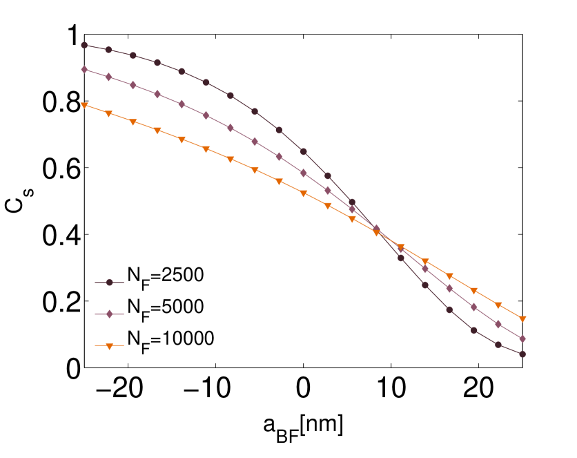
Figure 14: (Color online) Spatial correlation $C_{s}$ of the ground state of the 2D mixture as a a function of $a_{\mathrm{BF}}$, for three values of the number of fermions. The other parameters are: $N_{\mathrm{B}}=5\times 10^{4}$, $a_{\mathrm{B/F}}=5$ nm, $\omega_{x,\mathrm{B/F}}=\omega_{y,\mathrm{B/F}}=30$ Hz and $\omega_{z,\mathrm{B/F}}=1000$ Hz. Fermions are in the fully polarized state.

The Fig. 15 shows the spatial correlation, defined as per Eq. (36), for the three fermionic regimes: polarized, BCS and unitarity. The figure is a counterpart of Fig. 10 drawn for the 1D case, but only for the spatial correlation in the GS ($C_{s}$). One may conclude that these fermionic regimes show the behavior similar ti that observed in the 1D case, a difference being that the three curves demonstrate stronger demixing when $a_{\mathrm{BF}}$ changes from positive to negative values. In the unitarity regime it is again observed that the correlation reaches a maximum close to $1$ at $a_{\mathrm{BF}}\approx-10$ nm, dropping to negative values when the mixture is strongly repulsive.

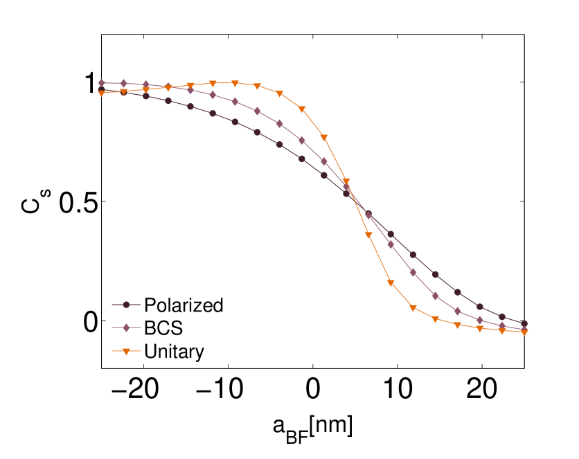
Figure 15: (Color online) Spatial correlation $C_{s}$ of the ground state of the 2D mixture as a a function of $a_{\mathrm{BF}}$, for three fermionic regimes: polarized, BCS, and unitarity. The fixed parameters are: $N_{\mathrm{B}}=5\times 10^{4}$, $N_{\mathrm{F}}=2.5\times 10^{3}$, $a_{\mathrm{B/F}}=5$ nm, $\omega_{x,\mathrm{B/F}}=\omega_{y,\mathrm{B/F}}=30$ Hz and $\omega_{z,\mathrm{B/F}}=1000$ Hz.

3.2.3 Accuracy of the variational method for the spatiotemporal dynamic

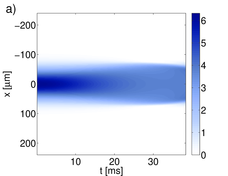
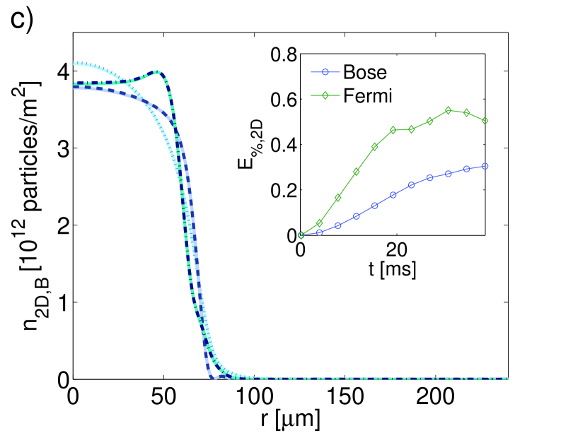
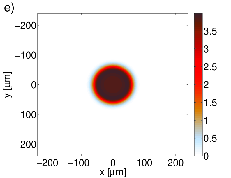
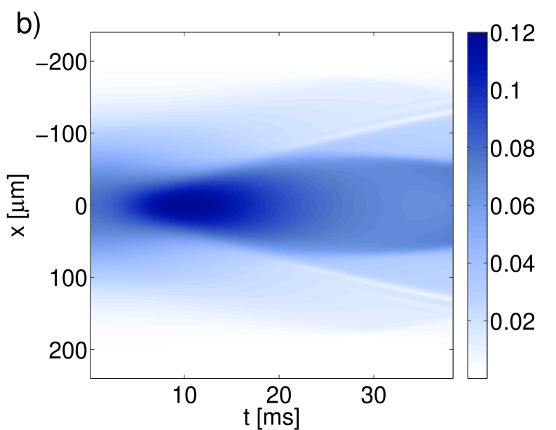
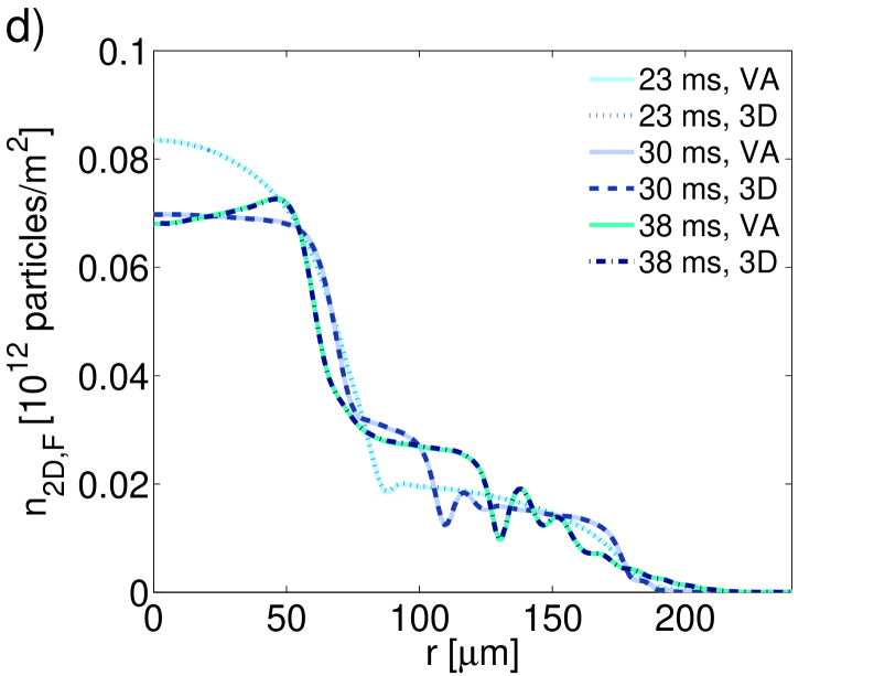
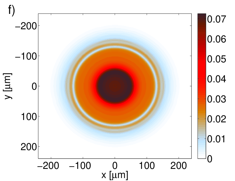
Figure 16: (Color online) 2D dynamics, as produced by the 2D VA, and by the 3D simulations for the attractive mixture of bosons (above) and fermions (below). Spatiotemporal diagrams (a) and (b), produced by the 3D simulations, show how the profiles of the densities of particles in the $x$ direction evolve in time (it is a cut of the 2D density with cylindrical symmetry). The curves in panels (c) and (d) shows the radial profiles for three different instants of time (see the inset in panel (d)), as produced by both the VA and 3D simulations. Diagrams (e) and (f) show 2D densities in the $xy$-plane for the last moments of time in panels (a) and (b). The inset in panel (c) shows the evolution of 2D error ($E_{\%,\mathrm{2D}}$) in time. Initial conditions are described in the text, and parameters are the same as in Fig. 12 with $a_{\mathrm{BF}}=-12nm$.

Figure 16 shows, for the attractive mixture ($g_{\mathrm{BF}}=-12nm$), the comparison between the results obtained by the t3D integration (Eqs. 5 and 6) with the results obtained by the 2D integration of the variational equations (Eqs. 30 and 31). The approach is similar to that developed in Sec. 3.1.4 for the 1D case. It starts from arbitrary initial conditions in 2D, viz., 2S fields with Gaussian shapes in the radial direction, a standard deviation of $50\mu m$ for bosons and $100\mu m$ for fermions being assumed. The initial conditions for the 3D dynamics are obtained with the ansatz given by Eq. 23 and assuming a Gaussian in the $xy$-plane. Panels 16(a) and 16(b) display two spatiotemporal diagrams, obtained from the 3D integration, showing a cut along the $x$ axis of the 2D density; since the dynamics, for the time range observed, obeys the cylindrical symmetry, this cut is representative. It is seen that the boson profile clearly affects the fermion profile. As the initial conditions do not correspond to the ground state, the fermions are attracted to the center by the bosonic pattern and are subject to the confinement imposed by the harmonic potential, generating strong interaction with the boson core. A gray soliton ring is generated (in panel 16(b) it is seen as a gray soliton). In panels 16(c) and 16(d), the radial profile obtained by the 3D integration and by VA for three instants of time are compared, showing that it is not possible to distinguish them. The inset in panel 16(c) shows that, in the observed range, the 2D overall error is less than $1\%$ (at initial time, it is zero because the 3D initial conditions are obtained from the 2D configuration using the ansatz, Eq. 23). The approach delivers very good results. In addition, in panel 16(d) it was observed that the rings are gray (the minimum value of the fermion density is not zero). Panels 16(e) and 16(f) show diagrams of the 2D density in the $xy$-plane for the last moment of time, highlighting the gray ring soliton observed in the fermionic component, which expands wherein the boson density is zero. We note that, in this case, the approximation is very good and allows one to considerably reduce the computing time needed to observe the 2D dynamics. The dynamics of the mixture thus produces a vast variety of localized nonlinear structures.

4 Conclusions

The incorporation of the width of the confined species as a variational variable shows that the term accounting for the interaction between the bosonic and fermionic species in the lower-dimensional equations is inversely proportional to the width in the confined direction(s). The derived systems of equations, which include the algebraic equations for the widths as functions of the 1D or 2D bosonic and fermionic densities. These approximations yield solutions which agree well with the full 3D theory. It is worthy to note that the ensuing relation between the widths and densities significantly varies with the strength of the inter-species interaction, which can be tuned by means of the Feshbach resonance. For very low densities, our equations are similar to the simplest models which postulate constant confinement width in the transverse direction(s). As an application of the variational method, we have studied the spatial correlation between the species, in which a strong dependence on the interaction parameter was observed. This sensitivity becomes stronger for the repulsive interaction, which causes demixing of the species.

It was observed too that, in 1D and 2D alike, the spatial correlation between the species is also strongly affected by the inter-species interaction strength. In addition, it was concluded that the greatest contrasts in the correlation, changing from the large correlation in the highly attractive mixtures to a weak correlation in the strongly repulsive ones, occur in the unitarity fermionic regime. Further, in the 1D setting the dynamics near the ground state demonstrates that the spatiotemporal correlation follows the same trends as the spatial correlation, the largest (but still small) difference being observed for strongly repulsive mixtures

Finally, it is relevant to mention that the mixture can also give rise to stable dark solitons in the Fermi field, in both the 1D and in 2D cases. However, as the hydrodynamic conditions was assumed, the solitons may occur in some form but are unconfirmed and should not be believed in too strongly. A detailed characterization of these states and the validity of the hydrodynamic approximation for them will be presented elsewhere.

References

References

- [1] Bloch I, Dalibard J, and Zwerger W 2008 Rev. Mod. Phys. 80 885
- [2] Giorgini S, Pitaevskii L P, and Stringari S 2008 Rev. Mod. Phys. 80 1215
- [3] Yukalov V I 2009 Laser Physics 19 1
- [4] Dalibard J, Gerbier J, Juzeliūnas G, and Öhberg P 2011 Rev. Mod. Phys. 83 1523
- [5] Hauke P, Cucchietti F M, Tagliacozzo L, Deutsch I, and Lewenstein M 2012 Rep. Prog. Phys. 75 08240
- [6] Bloch I, Dalibard J, and Nascimbène S 2012 Nature Phys. 8 267
- [7] Zhai H 2012 Int. J. Mod. Phys. B 26 123001
- [8] Zhou X, Li Y, Cai Z, and Wu C 2013 J. Phys. B: At. Mol. Opt. Phys. 46 134001
- [9] Truscott A G, Strecker K E, McAlexander W I, Partridge G B, Hulet R G 2001 Science 291 2570
- [10] Schreck F, Khaykovich L, Corwin K L, Ferrari G, Bourdel T, Cubizolles J, and Salomon C 2001 Phys. Rev. Lett.87 08040
- [11] Hansen A H, Khramov A, Dowd W H, Jamison A O, Ivanov V V, and Gupta S 2011 Phys. Rev. A 84 011606(R)
- [12] Heinze J, Götze S, Krauser J S, Hundt B, Fläschner N, Lühmann D-S, Becker C, and Sengstock K 2011 Phys. Rev. Lett. 107 135303
- [13] Tey M K, Stellmer S, Grimm R, and Schreck F 2010 Phys. Rev. A 82 011608(R)
- [14] Best Th, Will S, U. Schneider U, Hackermüller L, van Oosten D, and Bloch I 2009 Phys. Rev. Lett. 102 030408
- [15] Cumby T D, Shewmon R A, Hu M-G, Perreault J D, and Jin D S 2013 Phys. Rev. A 87 012703
- [16] Deh B, Gunton W, Klappauf B G, Li Z, Semczuk M, Van Dongen J, and Madison K W 2010 Phys. Rev. A 82 020701(R)
- [17] Tung S-K, Parker C, Johansen J, and Chin C 2013 Phys. Rev. A 87 010702(R)
- [18] Park J W, Wu C-H, Santiago I, Tiecke T G, Will S, Ahmadi P, and Zwierlein M W 2012 Phys. Rev. A 85 051602(R)
- [19] Wu C-H, Santiago I, Park J W, Ahmadi P, and Zwierlein M W 2011 Phys. Rev. A 84 011601(R)
- [20] Lelas K, Juki D and Buljan H 2009 Phys. Rev. A 80 053617
- [21] Watanabe T, Suzuki T, and Schuck P 2008 Phys. Rev. A 78 033601
- [22] Kain B and Ling H Y 2011 Phys. Rev. A 83 061603(R)
- [23] Mering A and Fleischhauer M 2011 Phys. Rev. A 83 063630
- [24] Song J-L and Zhou F 2011 Phys. Rev. A 84 013601
- [25] Ludwig D, Floerchinger S, Moroz S, and Wetterich C 2011 Phys. Rev. A 84 033629
- [26] Bertaina G, Fratini E, Giorgini S, and Pieri P 2013 Phys. Rev. Lett. 110 115303
- [27] Adhikari S K, and Salasnich L 2008 Phys. Rev. A 78 043616
- [28] Maruyama T and Yabu H 2009 Phys. Rev. A 80 043615
- [29] Iskin M and Freericks J K 2009 Phys. Rev. A 80 053623
- [30] Snoek M, Titvinidze I, Bloch I, and Hofstetter W, Phys. Rev. Lett. 106 155301
- [31] Nishida Y and Son D T 2006 Phys. Rev. A 74 013615
- [32] Salasnich L and Toigo F 2007 Phys. Rev. A 75 013623
- [33] Gautam S, Muruganandam P, and Angom D 2011 Phys. Rev. A 83 023605
- [34] Salasnich L, Adhikari S K, and Toigo F 2007 Phys.Rev. A 75 023616
- [35] Adhikari S K, and Salasnich L 2007 Phys. Rev. A76 023612
- [36] Yin X, Chen S, and Zhang Y 2009 Phys. Rev. A 79 053604
- [37] Lü X, Yin X, and Zhang Y 2010 Phys. Rev. A 81 043607
- [38] Qi P-T and Duan W-S 2011 Phys. Rev. A 84 033627
- [39] Das K K 2003 Phys. Rev. Lett. 90 170403
- [40] Fang B, Vignolo P, Gattobigio M, Miniatura C, and Minguzzi A 2011 Phys. Rev. A 84 023626
- [41] Abdullaev F Kh, Ögren M, and Sørensen M P 2013 Phys. Rev. A 87 023616
- [42] Adhikari S K, Malomed B A, Salasnich L, and Toigo F 2010 Phys. Rev. A 81 053630
- [43] Cheng Y, and Adhikari S K 2011 Phys. Rev. A 84 023632
- [44] Salasnich L, Parola A, and Reatto L 2002 Phys. Rev. A 65 043614
- [45] Díaz P, Laroze D, Malomed B A and Schmidt I 2012 J. Phys. B 45 145304
- [46] Manini N and Salasnich L 2005 Phys. Rev. A 71 033625
- [47] Salasnich L and Toigo F 2009 Phys. Rev. A 78 053626
- [48] Ancilotto F, Salasnich L, and Toigo F 2009 Phys. Rev. A 79 033627
- [49] Ancilotto F, Salasnich L, and Toigo F 2012 Phys. Rev. A 85 063612
- [50] Huang K and Yang C N 1957 Phys. Rev. 105 767
- [51] Lee T D and Yang C N 1957 Phys. Rev. 105 1119.
- [52] Adhikari S K and Malomed B A 2006 Phys. Rev. A 74 053620
- [53] Adhikai S K and Malomed B A 2009 Physica D 238 1402
- [54] Bragard J, Boccaletti S, Mendoza C, Hentschel H G E, and Mancini H 2004 Phys. Rev. E 70 036219
- [55] Cardoso W B, Zeng J, Avelar A T, Bazeia D, and Malomed B A 2013 Phys. Rev. E 88 025201
- [56] Scott R G, Dalfovo F, Pitaevskii L P, and Stringari S 2011 Phys. Rev. Lett. 106 185301
- [57] Yefsah T, Sommer A T, Ku M J H, Cheuk L W, Ji W, Bakr W S and Zwierlein M W 2013 Nature 499 426-430
- [58] Shomroni I, Lahoud E, Levy S, and Steinhauer J 2009 Nature Phys. 5 193-197
- [59] Sacha K, and Delande D 2014 Phys. Rev. A 90 021604(R)
- [60] Donadello S, Serafini S, Tylutki M, Pitaevskii L P, Dalfovo F, Lamporesi G, and Ferrari G 2014 Phys. Rev. Lett. 113 065302