A posteriori error estimates for discontinuous Galerkin methods using non-polynomial basis functions.
Part I: Second order linear PDE’s

Abstract

abstract

1 Numerical results

In this section we test the effectiveness of the a posteriori error estimators. The test program is written in MATLAB, and all results are obtained on a 2.7 GHz Intel processor with 16 GB memory. All numerical results are performed using the symmetric bilinear form ($\theta=1$). The effectiveness of the upper bound and lower bound on the global domain will be justified by comparing $|\!|\!|u-u_{N}|\!|\!|$ and $\eta$, and by comparing $|\!|\!|u-u_{N}|\!|\!|$ and $\xi$, respectively. It should be noted that although our theory does not directly predict the effectiveness of the estimator on each local element $\kappa$, we can measure the local effectiveness of the upper and lower bound on each local element $\kappa$ by defining

$$C_{\eta}(\kappa)=\frac{\eta_{{\tt R},\kappa}+\eta_{{\tt F},\kappa}+\eta_{{\tt J},\kappa}}{|\!|\!|u-u_{N}|\!|\!|_{\kappa}},\quad C_{\xi}(\kappa)=\frac{\xi_{\kappa}}{|\!|\!|u-u_{N}|\!|\!|_{\kappa}},$$ (1)

where the broken energy norm $|\!|\!|u-u_{N}|\!|\!|_{\kappa}$ is defined according to Eq. (LABEL:eq:DGnorm).

The numerical results are organized as follows. In section 1.1, we apply the general approach developed in section LABEL:sec:computation to compute the constants ${\tt a}_{\kappa},{\tt b}_{\kappa},{\tt d}_{\kappa}$ for polynomial basis functions, and verify that the scaling properties of the numerically computed constants match the analytic results known in the literature [Schwab1998]. In section 1.2, we illustrate the behavior of the upper bound and the lower bound error estimates for second order PDEs associated with positive definite operators. We then demonstrate the results for indefinite operators in section 1.3. In the a posteriori error estimates of both the upper bound and the lower bound, we make the assumption that the non-computable number ${\tt d}_{\kappa}^{u}(u_{N})$ can be approximated by ${\tt d}_{\kappa}$ without significant loss of effectiveness. We justify such treatment in section 1.4 by directly calculating ${\tt d}_{\kappa}^{u}(u_{N})$ using the numerically computed reference solution.

Our test problems include both one dimensional (1D) and two dimensional (2D) domains with periodic boundary conditions. Our non-polynomial basis functions are generated from the adaptive local basis (ALB) set [LinLuYingE2012] in the DG framework. The ALB set was originally proposed to systematically reduce the number of basis functions used to solve Kohn-Sham density functional theory calculations, and in this section we demonstrate its usage to solve second order linear PDEs. We denote by $N$ the number of ALBs per element. For operators in the form of $A=-\Delta+V$ with periodic boundary condition, the basic idea of the ALB set is to use eigenfunctions computed local domains as basis functions corresponding to the lowest few eigenvalues. The eigenfunctions are associated with the same operator $A$, but with modified boundary conditions on the local domain. More specifically, in a $d$-dimensional space, for each element $\kappa$, we form an extended element $\widetilde{\kappa}$ consisting of $\kappa$ and its $3^{d}-1$ neighboring elements in the sense of periodic boundary condition. On $\widetilde{\kappa}$ we solve the eigenvalue problem

$$-\Delta\widetilde{\varphi}_{i}+V\widetilde{\varphi}_{i}=\lambda_{i}\widetilde{\varphi}_{i}.$$ (2)

with periodic boundary condition on $\partial\widetilde{\kappa}$. This eigenvalue problem can be solved using standard basis set such as finite difference, finite elements, or planewaves. Here we solve the local eigenvalue problem (2) using planewaves which naturally satisfy periodic boundary conditions. Since this eigenvalue problem is solved on a extended element $\widetilde{\kappa}$ the computational cost is not large. The collection of eigenfunctions (corresponding to lowest $N$ eigenvalues) are restricted from $\widetilde{\kappa}$ to $\kappa$, i.e.

$$\varphi_{i}(x)=\begin{cases}\left[\widetilde{\varphi}_{i}\right]|_{\kappa}(x),&x\in\kappa;\\ 0,&\text{otherwise}.\end{cases}$$

After orthonormalizing $\{\varphi_{i}\}$ locally on each element $\kappa$ and removing the linearly dependent functions, the resulting set of orthonormal functions are called the ALB functions.

Since periodic boundary condition is used on the global domain $\Omega$, in all the calculations, the reference solution, which can be treated as a numerically exact solution, is solved using a planewave basis set with a sufficiently large number of planewaves. The ALB basis set is also computed using a sufficiently large number of planewaves on the extended element $\widetilde{\kappa}$. Then a Fourier interpolation procedure is carried out from $\widetilde{\kappa}$ to the local element $\kappa$ on a Legendre-Gauss-Lobatto (LGL) for accurate numerical integration.

1.1 Estimating the constants for polynomial basis functions

Although the main purpose of this paper is to design a posteriori error estimator for non-polynomial basis functions, the computational strategies discussed in section LABEL:sec:computation can be applied to polynomial functions as well. Let $\kappa=[0,h]^{d}$ and $\mathbb{V}_{N}(p;\kappa)=\text{span}\{\prod_{l=1}^{d}x_{l}^{j_{l}},j_{l}\in\mathbb{N},\sum_{l=1}^{d}j_{l}\leq p\}$ be the space spanned by polynomials with degree less than or equal to $p$. Then the asymptotic scaling of ${\tt a}_{\kappa},{\tt b}_{\kappa},{\tt d}_{\kappa}$ with respect to $h$ and $p$ is known [HoustonSchotzauWihler2007]

$${\tt a}_{\kappa}^{2}\sim\frac{h^{2}}{p^{2}},\quad{\tt b}_{\kappa}^{2}\sim\frac{h}{p},\quad{\tt d}_{\kappa}^{2}\sim\frac{p^{2}}{h}.$$ (3)

These results are asymptotically correct as $p\to\infty$, and we will show that the strategy discussed in section LABEL:sec:computation leads to the same asymptotic result, but the result is more accurate in the pre-asymptotic regime due to the explicit computation of the constants.

From numerical point of view, the scaling with respect to $h$ is naturally satisfied. To verify this, we can simply consider a reference element $\kappa|_{h=1}=[0,1]^{d}$ and scale the weight matrix $W^{[d]}$ and the differentiation matrix $D_{l}^{[d]}$ accordingly. The technique is the same as that used in [Schwab1998].

We now directly verify the scaling with respect to $p$ in Fig. 1, using the algorithms presented in section LABEL:sec:computation. The LGL grid sizes for 1D, 2D and 3D calculation are chosen to be $100$, $100\times 100$, and $50\times 50\times 50$, respectively. The largest degree of polynomials is $64$ for 1D and 2D, and is $16$ for the 3D case. Note that in the 3D case, the dimension of $\mathbb{V}_{N}(p=16;\kappa)$ is already $969$. Fig. 1 (a) shows the behavior of ${\tt a}_{\kappa}^{2}$, which asymptotically agrees with the $1/p^{2}$ scaling. It is interesting to see that the computed ${\tt a}_{\kappa}^{2}$ can be approximated by $C\frac{h^{2}}{p^{2}}$ where the constant $C$ is around $0.1$. The recovery of the constant indicates that the numerically computed constant ${\tt a}_{\kappa}$ can offer a sharper estimator even for the standard $hp$-refinement. Similarly Fig. 1 (b) shows that ${\tt b}_{\kappa}^{2}$ asymptotically scales as $1/p$ for 2D and 3D simulation. The 1D case is not shown in the picture, since the numerical value of ${\tt b}_{\kappa}^{2}$ is already as small as $10^{-20}$ for $p=2$. This can be interpreted from Proposition LABEL:prop:rbk1D in the appendix. Finally, direct computation in Fig. 1 (c) shows that ${\tt d}_{\kappa}^{2}$ asymptotically scales as $p^{2}$ for all dimensions. Again, the computed constant ${\tt d}_{\kappa}^{2}$ differs from the asymptotic scaling in the pre-asymptotic regime, indicating that the numerically computed constant should be sharper for low order polynomials ($p\leq 4$).

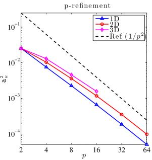
(a) (a)

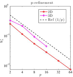
(b) (b)

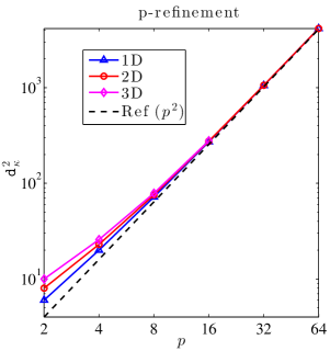
(c) (c)

Fig. 1: Numerically computed constants ${\tt a}_{\kappa}^{2},{\tt b}_{\kappa}^{2},{\tt d}_{\kappa}^{2}$ with respect to the polynomial degrees $p$ in 1D, 2D and 3D.

1.2 Positive definite operators

We first demonstrate the effectiveness of the a posteriori error estimates for a positive definite operator on a 1D domain $\Omega=(0,2\pi)$, using the ALB set as non-polynomial basis functions. Due to the periodic boundary condition, we choose $V(x)=0.01$ so that the operator $A=-\Delta+V$ is non-singular and positive definite. The right hand side is chosen to be $f(x)=\sin(6x)$ which is periodic on $\Omega$. In the ALB computation, the domain is partitioned into $7$ elements, as indicated by black dashed lines. Fig. 2 shows solution $u$ to Eq. (LABEL:eq:Indef) and the point-wise error $u-u_{N}$ using $N=11$ ALBs per element.

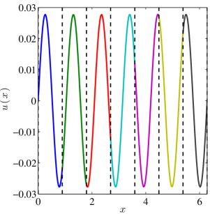
(a) (a)

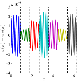
(b) (b)

Fig. 2: (a) The reference solution $u(x)$ corresponding to $V(x)=0.01$ and the right hand side $f(x)=\sin(6x)$. (b) Point-wise error between the reference solution $u(x)$ and the numerical solution $u_{N}(x)$ calculated using the ALB set with $7$ elements and $N=11$ basis functions per element. The domain is partitioned into $7$ elements indicated by black dashed lines.

Fig. 3 (a) shows the absolute error in the energy norm, the upper bound and lower bound estimates as the number of ALBs per element $N$ increases from $3$ to $15$. The relative error can be deduced by comparing Fig. 3 (a) and Fig. 2 (a). We find that the computed $\eta$ and $\xi$ are indeed upper and lower bounds of the true error $|\!|\!|u-u_{N}|\!|\!|$ for all $N$ across a wide range of accuracy (from $10^{-1}$ to $10^{-8}$). It also appears that the lower bound estimator $\xi$ follows the true error more closely than the upper bound estimator $\eta$. Fig. 3 (b) and (c) illustrate the local effectiveness $C_{\eta}(\kappa)$ and $C_{\xi}(\kappa)$ for each element $\kappa$. Though not guaranteed by our theory, we observe that $\eta_{\kappa}$ and $\xi_{\kappa}$ are upper and lower bounds for $|\!|\!|u-u_{N}|\!|\!|_{\kappa}$ for each element $\kappa$, respectively. The effectiveness as measured by $C_{\eta}(\kappa)$ and $C_{\xi}(\kappa)$ depends only weakly on the number of adaptive local basis functions, or the accuracy of the numerical solution.

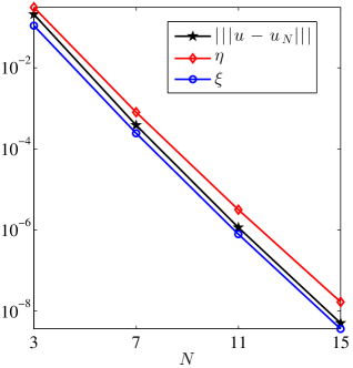
(a) (a)

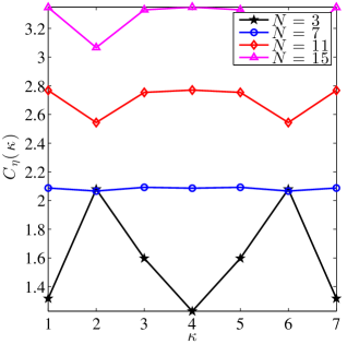
(b) (b)

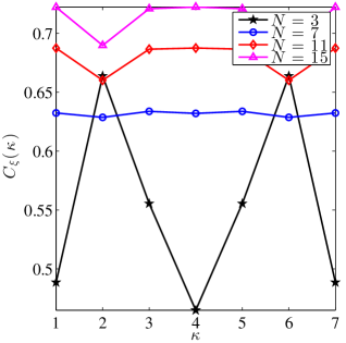
(c) (c)

Fig. 3: (a) Global error and the upper/lower bound estimator for $V(x)=0.01$ and $f(x)=\sin(6x)$. (b) Local effectiveness of the upper bound characterized by $C_{\eta}(\kappa)$ for each element. (c) Local effectiveness of the lower bound characterized by $C_{\xi}(\kappa)$ for each element.

Our next example is to solve a 2D problem with $\Omega=(0,2\pi)\times(0,2\pi)$. Again we choose $V(x,y)=0.01$ so that $A=-\Delta+V$ is non-singular and positive definite. The right hand side is $f(x,y)=\cos(3x)\cos(y)$, which satisfies the periodic boundary condition. Fig. 4 shows the reference solution $u$ to Eq. (LABEL:eq:Indef) and the point-wise error $u-u_{N}$ using $N=31$ ALBs per element. In the ALB computation, the domain is partitioned into $5\times 5$ elements, indicated by black dashed lines.

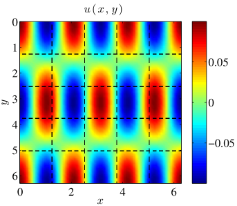
(a) (a)

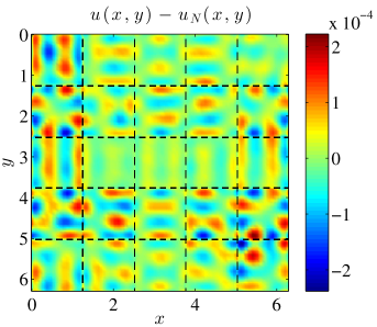
(b) (b)

Fig. 4: (a) The reference solution $u(x,y)$ corresponding to $V(x,y)=0.01$ and $f(x,y)=\cos(3x)\cos(y)$. (b) Point-wise error between the reference solution $u(x,y)$ and the numerical solution $u_{N}(x,y)$ calculated using the ALB set with $5\times 5$ elements and $N=31$ basis functions per element.

Fig. 5 (a) shows the error in the energy norm, the computed upper bound and the lower bound as the number of ALBs per element $N$ increases from $11$ to $41$. Both the computed upper and the lower bound estimates are effective for all calculations. Fig. 5 (b)-(d) illustrates the local effectiveness of the upper and lower bound estimates for the two extreme cases $N=11$ and $N=41$, and the estimator $\eta_{\kappa}$ and $\xi_{\kappa}$ are effective for all elements, and the effectiveness depends weakly on the number of basis functions per element.

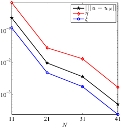
(a) (a)

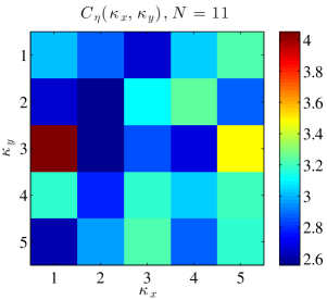
(b) (b)

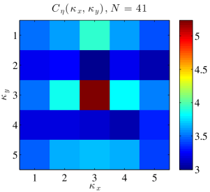
(c) (c)

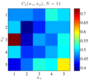
(d) (d)

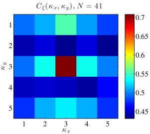
(e) (e)

Fig. 5: (a) Global error and the upper/lower bound estimator for $V(x,y)=0.01$ and $f(x,y)=\cos(3x)\cos(y)$. (b) Local effectiveness of the upper bound characterized by $C_{\eta}$ in each element for $N=11$. (c) Local effectiveness of the upper bound characterized by $C_{\eta}$ in each element for $N=41$. (d) Local effectiveness of the lower bound characterized by $C_{\xi}$ in each element for $N=11$. (e) Local effectiveness of the lower bound characterized by $C_{\xi}$ in each element for $N=41$.

1.3 Indefinite operators

We now demonstrate the effectiveness of the upper and lower bound estimates for indefinite operators. We start from a 1D example on a domain $\Omega=(0,2\pi)$ with periodic boundary conditions. The potential function $V(x)$ is given by the sum of three Gaussians with negative magnitude, as shown in Fig. 6 (a). The operator $A=-\Delta+V$ has $3$ negative eigenvalues and is indefinite. The right hand side is $f(x)=\sin(6x)$. The domain is partitioned into $7$ elements for the ALB calculation. Fig. 6 (b) shows the reference solution $u$ to Eq. (LABEL:eq:Indef), and Fig. 6 (c) shows the point-wise error $u-u_{N}$ using $N=11$ ALBs per element.

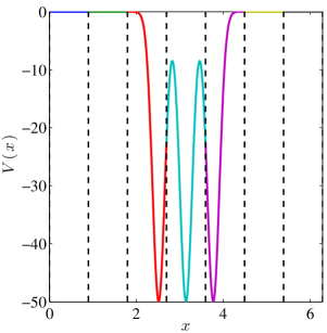
(a) (a)

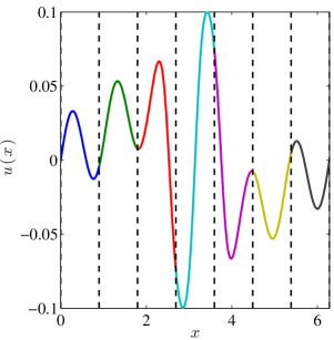
(b) (b)

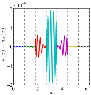
(c) (c)

Fig. 6: (a) The potential $V(x)$ given by the sum of three Gaussians with negative magnitude. (b) The reference solution $u(x)$ corresponding to the potential $V(x)$ in (a) and the right hand side $f(x)=\sin(6x)$. (c) Point-wise error between the reference solution $u(x)$ and the numerical solution $u_{N}(x)$ calculated using the ALB set with $7$ elements and $N=11$ basis functions per element.

Fig. 7 (a) shows the error in the energy norm, the computed upper and lower bound estimates as the number of ALBs per element $N$ increases from $3$ to $15$. Similar to Fig. 3, the computed $\eta$ and $\xi$ are upper and lower bounds for the true error $|\!|\!|u-u_{N}|\!|\!|$ for all $N$ across a wide range of accuracy. Furthermore, the computed $\xi$ is always a lower bound of $|\!|\!|u-u_{N}|\!|\!|$ from $N=3$ to $N=15$. This is guaranteed by the property of the lower bound in Proposition LABEL:prop:GlobLowerBound.

We should note that when the number of basis functions is very small ($N=3$), the accuracy is low and the ALB approximation is in its pre-asymptotic regime. In such case, the upper bound is very close to the true error. In fact as indicated by Theorem LABEL:thm:IndefApost, $\eta$ may not even be a rigorous upper bound for highly indefinite operators with very few basis functions.

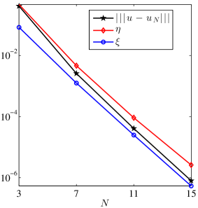
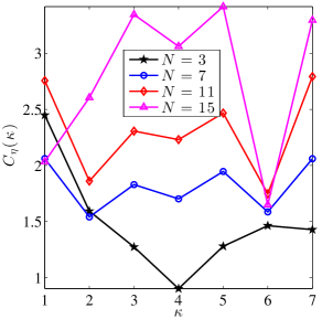
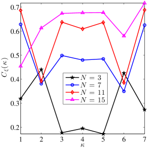
Fig. 7: (a) Global error and the upper/lower bound estimator for $V(x)$ given in Fig. 6 (a) and $f(x)=\sin(6x)$. (b) Local effectiveness of the upper bound characterized by $C_{\eta}$ in each element. (c) Local effectiveness of the lower bound characterized by $C_{\eta}$ in each element.

Our final examples are two indefinite problems on a 2D domain $\Omega=(0,2\pi)\times(0,2\pi)$. The first problem is a homogeneous Helmholtz equation with $V(x,y)=-16.5$ and the operator $A=-\Delta+V$ has $49$ negative eigenvalues. The right hand side is

$$f(x,y)=\exp(-2(x-\pi)^{2}-2(y-\pi)^{2}),$$ (4)

which is a Gaussian located at the center of $\Omega$. The second problem is that $V$ is given by the sum of four Gaussians with negative magnitude, as illustrated in Fig. 10 (a). The operator $A=-\Delta+V$ has $26$ negative eigenvalues. The right hand side is chosen to be $f(x,y)=\cos(3x)\cos(y)$ satisfying the periodic boundary condition. For the first problem, Fig. 8 (b) shows the reference solution $u$ to Eq. (LABEL:eq:Indef) and Fig. 8 (c) shows the point-wise error $u-u_{N}$ using $N=31$ ALBs per element. In the ALB computation, the domain is partitioned into $5\times 5$ elements, indicated by black dashed lines. Similarly for the second problem, Fig. 10 shows solution $u$ to Eq. (LABEL:eq:Indef) and the point-wise error $u-u_{N}$ using $N=31$ ALBs per element.

Fig. 9 (a)-(e) illustrates the global and local effectiveness of the upper and lower bound estimates for the Helmholtz problem, as the number of ALBs per element $N$ increases from $21$ to $51$. Compared to the positive definite case in Fig. 5, the true error is larger using a comparable number of basis functions, reflecting that the Helmholtz equation is more difficult to solve. Nonetheless, $\eta$ and $\xi$ provide effective bounds for the true error in all cases. Similar results can be found for the indefinite example with negative Gaussian potentials in Fig. 11 (a)-(e). In all calculations, the computed lower bound estimator remains a lower bound for the true error. In particular, the estimators still hold quite tightly in the pre-asymptotic regime $(N=11)$ where the ALB approximation is crude and has large numerical error.

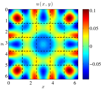
(a) (a)

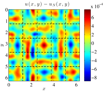
(b) (b)

Fig. 8: (a) The reference solution $u(x,y)$ corresponding to $V(x,y)=-16.5$ and $f(x,y)$ in Eq. (4), which is a Gaussian localized at the center of $\Omega$. (b) Point-wise error between the reference solution $u(x,y)$ and the numerical solution $u_{N}(x,y)$ calculated using the ALB set with $5\times 5$ elements and $N=31$ basis functions per element.

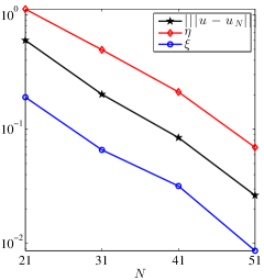
(a) (a)

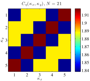
(b) (b)

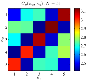
(c) (c)

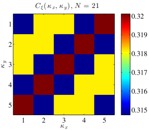
(d) (d)

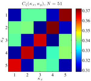
(e) (e)

Fig. 9: (a) Global error and the upper/lower bound estimator for $V(x,y)=-16.5$ and $f(x,y)$ in Eq. (4), which is a Gaussian localized at the center of $\Omega$. (b) Local effectiveness of the upper bound characterized by $C_{\eta}$ in each element for $N=21$. (c) Local effectiveness of the upper bound characterized by $C_{\eta}$ in each element for $N=51$. (d) Local effectiveness of the lower bound characterized by $C_{\xi}$ in each element for $N=21$. (e) Local effectiveness of the lower bound characterized by $C_{\xi}$ in each element for $N=51$.

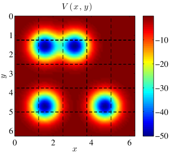
(a) (a)

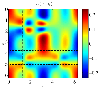
(b) (b)

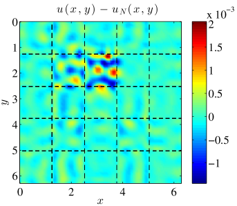
(c) (c)

Fig. 10: (a) The potential $V(x,y)$ four Gaussians with negative magnitude. (b) Solution $u(x,y)$ corresponding to $V(x,y)$ given in (a) and $f(x,y)=\cos(3x)\cos(y)$. (c) Point-wise error between the reference solution $u(x,y)$ and the numerical solution $u_{N}(x,y)$ calculated using the ALB set with $5\times 5$ elements and $N=31$ basis functions per element.

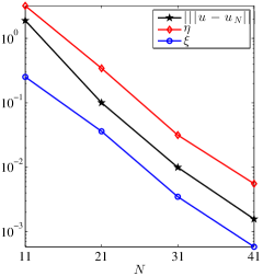
(a) (a)

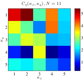
(b) (b)

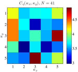
(c) (c)

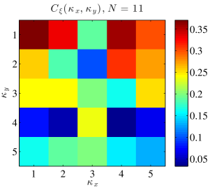
(d) (d)

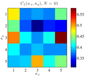
(e) (e)

Fig. 11: (a) Global error and the upper/lower bound estimator for $V(x,y)$ given in Fig. 10 (a) and $f(x,y)=\cos(3x)\cos(y)$. (b) Local effectiveness of the upper bound characterized by $C_{\eta}$ in each element for $N=11$. (c) Local effectiveness of the upper bound characterized by $C_{\eta}$ in each element for $N=41$. (d) Local effectiveness of the lower bound characterized by $C_{\xi}$ in each element for $N=11$. (e) Local effectiveness of the lower bound characterized by $C_{\xi}$ in each element for $N=41$.

1.4 Justification of the treatment of ${\tt d}_{\kappa}^{u}(u_{N})$

In the numerical computation of the upper and lower bound estimates, we approximated the non-computable constant ${\tt d}_{\kappa}^{u}(u_{N})$ by the computable constant ${\tt d}_{\kappa}$. Below we provide numerical justification of such approximation by direct computation of ${\tt d}_{\kappa}^{u}(u_{N})$ via the reference solution. We compare with ${\tt d}_{\kappa}$ and ${\tt b}_{\kappa}\gamma_{\kappa}$ since these three terms appear together in $\eta_{{\tt J},\kappa}$ in Eq. (LABEL:eq:Estim3).

Fig. 12 (a) and (b) compare ${\tt d}_{\kappa}^{u}(u_{N})$, ${\tt d}_{\kappa}$ and ${\tt b}_{\kappa}\gamma_{\kappa}$ for the positive definite and the indefinite 1D examples, respectively. We observe that the magnitude of ${\tt d}_{\kappa}^{u}(u_{N})$ is comparable to that of ${\tt d}_{\kappa}$. ${\tt b}_{\kappa}\gamma_{\kappa}$ is much smaller compared to ${\tt d}_{\kappa}^{u}(u_{N})$ and ${\tt d}_{\kappa}$. This is a direct consequence of Proposition LABEL:prop:rbk1D, which states that ${\tt b}_{\kappa}$ is in general very small for 1D systems.

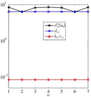
(a) (a)

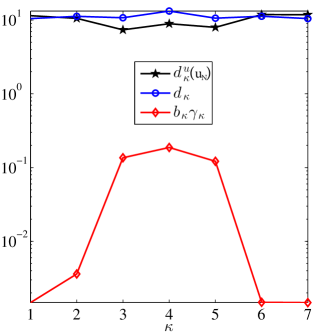
(b) (b)

Fig. 12: Comparison of ${\tt d}_{\kappa}^{u}(u_{N})$, ${\tt d}_{\kappa}$ and ${\tt b}_{\kappa}\gamma_{\kappa}$ for (a) the positive definite case with $V(x)=0.01$ with $N=7$. (b) the indefinite case with $V(x)$ given in Fig. 6 (a) with $N=7$.

Fig. 13 compare ${\tt d}_{\kappa}^{u}(u_{N})$, ${\tt d}_{\kappa}$ and ${\tt b}_{\kappa}\gamma_{\kappa}$ for the positive definite case $V=0.01$, the indefinite case $V=-16.5$, and the indefinite case with $V$ given by the sum of negative Gaussians in Fig. 10 (a). In all cases, the magnitude of ${\tt d}_{\kappa}^{u}(u_{N})$ is comparable to that of ${\tt d}_{\kappa}$. Furthermore, both ${\tt d}_{\kappa}^{u}(u_{N})$ and ${\tt d}_{\kappa}$ are much smaller compared to $\beta_{\kappa}\gamma_{\kappa}$. Therefore the effectiveness of the estimator remains unchanged even if ${\tt d}_{\kappa}^{u}(u_{N})$ is neglected. We expect similar results can be observed for systems of higher dimensionality.

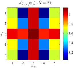
(a) (a)$V=0.01$

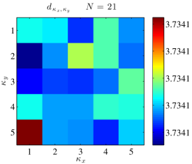
(b) (b)$V=0.01$

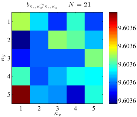
(c) (c)$V=0.01$

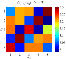
(d) (d)$V=-16.5$

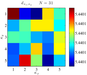
(e) (e)$V=-16.5$

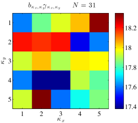
(f) (f)$V=-16.5$

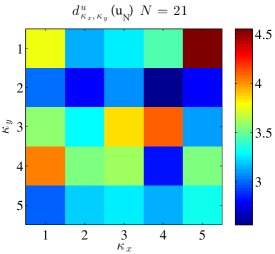
(g) (g)$V$ Gaussian

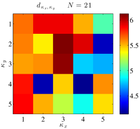
(h) (h)$V$ Gaussian

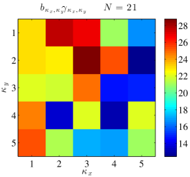
(i) (i)$V$ Gaussian

Fig. 13: Comparison of ${\tt d}_{\kappa}^{u}(u_{N})$, ${\tt d}_{\kappa}$ and ${\tt b}_{\kappa}\gamma_{\kappa}$ for 2D test problems for (a-c) the positive definite case $V=0.01$ (d-f) the indefinite case $V=-16.5$ (g-i) the indefinite case with $V$ given by the sum of negative Gaussians in Fig. 10 (a).

Finally we provide a second justification by comparing the total contribution of the jump term in the upper bound estimator

$$\eta_{J}^{2}=\sum_{\kappa}\eta_{J,\kappa}^{2},$$

and the total contribution of the jump term in the energy norm

$$E_{J}=\sum_{\kappa}\tfrac{\gamma_{\kappa}}{2}\|[\![u_{N}]\!]\|_{\partial\kappa}^{2}.$$

This is given in Table 1. It shows that the approximation $\REV{{\tt d}_{\kappa}^{u}(u_{N})}\approx{\tt d}_{\kappa}$ does not lead to underestimation of the jump term, which is consistent with the observation in Fig. 12 and 13.

Problem	$N$	$E_{J}$	$\eta_{J}^{2}$
1D $V=0.01$	$7$	$2.0179\times 10^{-8}$	$2.0182\times 10^{-8}$
2D $V=0.01$	$21$	$1.2030\times 10^{-5}$	$9.1593\times 10^{-5}$
1D Gaussian	$11$	$6.4687\times 10^{-11}$	$6.4697\times 10^{-11}$
2D $V=-16.5$	$31$	$4.7352\times 10^{-3}$	$5.6649\times 10^{-2}$
2D Gaussian	$21$	$1.6226\times 10^{-3}$	$2.8348\times 10^{-2}$

Table 1: Comparison of the total contribution of the jump term in the estimator $\eta_{J}^{2}$, and the total contribution of the jump term in the energy error $E_{J}$.