Fast Magnetic Reconnection Due to Anisotropic Electron Pressure

Abstract

A new regime of fast magnetic reconnection with an out-of-plane (guide) magnetic field is reported in which the key role is played by an electron pressure anisotropy described by the Chew-Goldberger-Low gyrotropic equations of state in the generalized Ohm’s law, which even dominates the Hall term. A description of the physical cause of this behavior is provided and two-dimensional fluid simulations are used to confirm the results. The electron pressure anisotropy causes the out-of-plane magnetic field to develop a quadrupole structure of opposite polarity to the Hall magnetic field and gives rise to dispersive waves. In addition to being important for understanding what causes reconnection to be fast, this mechanism should dominate in plasmas with low plasma beta and a high in-plane plasma beta with electron temperature comparable to or larger than ion temperature, so it could be relevant in the solar wind and some tokamaks.

Magnetic reconnection allows for large-scale conversion of magnetic energy into kinetic energy and heat by changing magnetic topology. It occurs in a wide range of environments, such as solar eruptions, planetary magnetospheres, fusion devices, and astrophysical settings Zweibel and Yamada (2009). One key unsolved problem is what determines the rate that reconnection proceeds Cassak and Shay (2012); Karimabadi et al. (2013).

In simplified two-dimensional (2D) systems often employed in simulations, the reconnection rate $E$ is determined by the aspect ratio of the current sheet, but it is not understood what controls its length. In collisional plasmas, current layers are elongated Sweet (1958); Parker (1957) which make collisional reconnection relatively slow. For less collisional 2D systems, elongated layers break and produce secondary islands Matthaeus and Lamkin (1986); Biskamp (1986); Loureiro et al. (2007); Bhattacharjee et al. (2009), giving normalized reconnection rates of 0.01 Bhattacharjee et al. (2009); Cassak et al. (2009); Huang and Bhattacharjee (2010). However, this is ten times slower than the fastest rates seen in simulations Daughton et al. (2009); Shepherd and Cassak (2010); Daughton and Roytershteyn (2012); Ji and Daughton (2011); Huang et al. (2011); Cassak and Drake (2013).

The GEM Challenge Birn et al. (2001) showed that the Hall term, when active, is sufficient to produce short current layers with $E\simeq 0.1$. The interpretation of this is still under debate Karimabadi et al. (2004a); Daughton et al. (2006); Drake et al. (2008); Malakit et al. (2009); Cassak et al. (2010); Liu et al. (2014); TenBarge et al. (2014). One can ask - do other mechanisms limit the length of current layers that could help explain what causes fast reconnection?

In this Letter, we report that fast reconnection can be caused by electron pressure anisotropy using the Chew-Goldberger-Low (CGL) equations of state Chew et al. (1956) in the generalized Ohm’s law. This has not been seen previously because (a) most simulations use no out-of-plane (guide) magnetic field, but this mechanism requires one and (b) previous fluid simulations included pressure anisotropies only in the momentum equation, which does not produce fast reconnection Birn and Hesse (2001); Hung et al. (2011); Meng et al. (2012). This result is distinguished from known results that off-diagonal elements of the electron pressure tensor balance the reconnection electric field at the reconnection site Vasyliunas (1975); Hesse et al. (1999); Hesse (2006) and agyrotropies contribute near the reconnection site Kuznetsova et al. (2001); Scudder and Daughton (2008). Neither effect is present for the CGL equations because the pressure tensor is gyrotropic. As with the Hall effect, gyrotropic pressure does not break the frozen-in condition Le et al. (2013). Nonetheless, it plays a crucial role in allowing fast reconnection in this regime.

Gyrotropic pressures are different parallel $p_{||}$ and perpendicular $p_{\perp}$ to the magnetic field Parker (1958). The CGL, or double adiabatic, equations of state Chew et al. (1956) follow rigorously from kinetic theory in the ideal limit (no heat conduction) with strong enough magnetic fields so particles are magnetized. Previous studies treated gyrotropic pressures in tearing instabilities Shi et al. (1987); Cai and Li (2009); Chen and Palmadesso (1984); Ambrosiano et al. (1986); Hesse and Winske (1994); Tanaka et al. (2011). Electron pressure anisotropies have garnered interest lately since they are self-generated by reconnecting magnetic field lines Egedal et al. (2013). The resulting equations of state Le et al. (2009) are valid for guide fields no stronger than the reconnecting magnetic field.

Simulations are carried out using the two-fluid code F3D Shay et al. (2004) modified to include gyrotropic pressures. The code updates the continuity equation, momentum equation, Faraday’s law, and pressure equations. The electric field ${\bf E}$ is given by the generalized Ohm’s law,

$${\bf E}+\frac{{\bf v}\times{\bf B}}{c}=\frac{{\bf J}\times{\bf B}}{nec}-\frac{1}{ne}\nabla\cdot{\bf p}_{e}+\eta{\bf J}+\frac{m_{e}}{e}\frac{d({\bf J}/ne)}{dt},$$ (1)

where ${\bf v}$ is velocity, ${\bf B}$ is magnetic field, ${\bf J}$ is current density, $n$ is number density, $e$ is proton charge, ${\bf p}_{e}$ is the electron pressure tensor, $\eta$ is resistivity, $m_{e}$ is electron mass, and each term on the right can be turned off, including the Hall term ${\bf J}\times{\bf B}/nec$. The momentum equation is

$$\frac{\partial(\rho{\bf v})}{\partial t}+\nabla\cdot(\rho{\bf v}{\bf v})=\nabla\cdot\left[\epsilon\frac{{\bf B}{\bf B}}{4\pi}-\left(p_{\perp}+\frac{B^{2}}{8\pi}\right){\bf I}\right],$$ (2)

where $\epsilon=1-4\pi(p_{||}-p_{\perp})/B^{2}$, ${\bf I}$ is the identity tensor, $\rho$ is mass density, and $p$ is total (electron plus ion) pressure.

When pressure anisotropies are used, we employ the CGL equations, equivalent to $p_{\sigma||}B^{2}/\rho^{3}$ and $p_{\sigma\perp}/\rho B$ being constants Chew et al. (1956) for species $\sigma$. We write them as evolution equations {see Eqs. (17) and (18) in Ref. Hesse and Birn (1992)} with ${\bf E}\cdot{\bf J}$ omitted for simplicity. The numerical implementation is benchmarked using Alfvén waves and the firehose and mirror instabilities. For isotropic plasmas, $p_{\sigma}/\rho^{5/3}$ = constant.

All quantities are normalized: magnetic fields to the reconnecting magnetic field $B_{0}$, densities to the value $\rho_{0}$ far from the current sheet, velocities to the Alfvén speed $c_{A}=B_{0}/(4\pi\rho_{0})^{1/2}$, lengths to the ion inertial length $d_{i}=c/\omega_{pi}$, electric fields to $c_{A}B_{0}/c$, resistivities to $4\pi c_{A}d_{i}/c^{2}$, and pressures to $B_{0}^{2}/4\pi$. The simulation size is $L_{x}\times L_{y}=204.8\times 102.4$ in a doubly periodic domain with 4096 $\times$ 2048 cells. This system is large enough that boundaries do not play a role; a steady state prevails for an extended time.

The initial reconnecting magnetic field is $B_{x}(y)=\tanh[(y+L_{y}/4)/0.5]-\tanh[(y-L_{y}/4)/0.5]-1$. Unless otherwise stated, the guide field is large at $5$ and increases at the current sheet to balance total pressure. The density $\rho=1$ and pressure $p_{\sigma}=5$ are initially uniform ($p_{\sigma\perp}=p_{\sigma||}=5$ for anisotropic). When electron pressure is evolved, ions are cold, and vice versa.

All simulations use $m_{e}=m_{i}/25$ unless otherwise stated, which is acceptable because $E$ is insensitive to $m_{e}$ Shay et al. (1998) and length scales for the ions ($c_{s}/\Omega_{ci}\simeq 0.7$) and electrons ($d_{e}=c/\omega_{pe}=0.2$) are sufficiently separated Cassak et al. (2007). The resistivity is 0.005, chosen so that if reconnection is Sweet-Parker-like, the layer thickness is $(\eta L_{x}/4)^{1/2}\simeq 0.5$ which makes it marginal against secondary islands Biskamp (1986). Reconnection is seeded using a coherent magnetic perturbation of amplitude $0.014$. Initial random velocity perturbations of amplitude 0.04 break symmetry. The equations employ fourth order diffusion with coefficient $D_{4}=2.5\times 10^{-5}$ to damp noise at the grid.

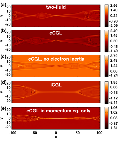
Figure 1: (Color) Out-of-plane current density $J_{z}$ using various models: (a) two-fluid, (b) eCGL, (c) eCGL with no electron inertia, (d) iCGL, (e) eCGL in the momentum equation only.

Benchmark simulations using two-fluid simulations (with the Hall term, electron inertia, and isotropic electron pressure) reveal a well-known open exhaust, as shown by the out-of-plane current density $J_{z}$ in Fig. 1(a). Various simulations are then performed without the Hall term. When the CGL equations are used on the electrons (which we call eCGL), an open exhaust occurs (panel b). Panel (c) is for the same system but with $m_{e}=0$, showing that electron inertia does not cause the open exhaust. Panel (d) is when the CGL equations are used on the ions (which we call iCGL). The current sheet is elongated like in Sweet-Parker reconnection. To further identify the key physics, a simulation of an unphysical system is tested: the electron pressure anisotropy is included in the momentum equation [Eq. (2)] but not in generalized Ohm’s law [Eq. (1)]. The result is an elongated current sheet (panel e). The three with open exhausts are fast, $E\simeq 0.06-0.1$, while the elongated sheets give the Sweet-Parker rate of 0.01. The thickness of the current sheets in (a) and (b) are near 0.2, showing that layers in eCGL go down to $d_{e}$ as in two-fluid reconnection. In contrast, the layer thickness for (d) and (e) is 0.525 and 0.6 (the Sweet-Parker thickness). The conclusion is clear: the eCGL equations give rise to fast reconnection even with no Hall term, and the key physics is the electron pressure gradient in generalized Ohm’s law.

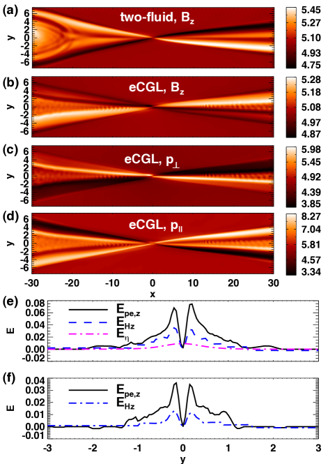
Figure 2: (Color) (a) Out-of-plane magnetic field $B_{z}$ in two-fluid reconnection. For eCGL simulation, (b) out-of-plane magnetic field $B_{z}$, (c) perpendicular electron pressure $p_{e\perp}$, and (d) parallel electron pressure $p_{e||}$. Reconnection electric field contributions in the (e) eCGL, two-fluid, and iCGL simulations and (f) a simulation with eCGL and the Hall term.

The physics when electron pressure anisotropies dominate bears similarities to Hall reconnection with a guide field Kleva et al. (1995). The $z$ component of Eq. (1) in terms of the flux function $\psi$ defined as $E_{z}=(1/c)\partial\psi/\partial t$ is

$$\frac{\partial\psi}{\partial t}+\left({\bf v}-\frac{{\bf J}}{ne}\right)\cdot\nabla\psi=-\frac{c}{ne}(\nabla\cdot{\bf p}_{e})_{z}+\left(\frac{\eta c^{2}}{4\pi}+\frac{d}{dt}d_{e}^{2}\right)\nabla^{2}\psi.$$ (3)

With the Hall term present, the left side reveals magnetic flux is convected by electrons, so electrons carrying the current drag the reconnecting magnetic field out of the plane Mandt et al. (1994). This produces a quadrupole out-of-plane magnetic field $B_{z}$ Sonnerup (1979), shown for the two-fluid simulation in Fig. 2(a). With a strong guide field, the gas pressure (not shown) develops a quadrupole with opposite polarity to maintain total pressure balance Kleva et al. (1995).

Without the Hall term, Eq. (3) implies magnetic flux is convected by ions Karimabadi et al. (2004b). The magnetic field is dragged out of the plane by ions, giving a $B_{z}$ quadrupole with opposite polarity as in Hall reconnection, displayed for the eCGL simulation in Fig. 2(b). (An instability is visible in the exhaust. The system is not firehose or mirror unstable; it is likely a drift instability.) To balance total pressure, $p_{e\perp}$ develops a quadrupole of opposite polarity, displayed in Fig. 2(c). The density (not shown) develops a quadrupole like that of $p_{e\perp}$. This requires a parallel electric field pointing from low density to high, which comes from a parallel electron pressure with high $p_{e||}$ in regions of low $p_{e\perp}$ so $p_{e||}$ has a quadrupole of opposite polarity as $p_{e\perp}$, shown in Fig. 2(d). Thus, an electron pressure anisotropy is self-generated. It contributes to the reconnection electric field as $E_{pe,z}=-(1/ne)(\nabla\cdot{\bf p}_{e})_{z}=-(1/ne)({\bf B}\cdot\nabla)[(p_{e\perp}-p_{e||})B_{z}/B^{2}]$, plotted as the solid line in a vertical cut through the X-line in Fig. 2(e). For comparison, the dashed line shows the Hall electric field $E_{Hz}$ in the two-fluid simulation and the dash-dot line shows the resistive electric field $E_{\eta}$ in the iCGL simulation. The structure of $E_{pe,z}$ is similar to the known $E_{Hz}$ profile in two-fluid reconnection. Note that eCGL with $m_{e}=0$ also has quadrupoles, but iCGL with slow reconnection does not.

The guide field is key to the physics. If it is too large, the ion Larmor radius falls below electron or resistive scales which prevents fast reconnection, analogous to Hall reconnection Aydemir (1992). If it is too small, the pressure change due to the $B_{z}$ quadrupole is small, so the effect in the previous paragraph is negligible. We quantify this by finding when $E_{pe,z}$ is dominated by other contributions to Ohm’s law, which for the present simulations is the resistive term. A scaling analysis gives $E_{pe,z}/E_{\eta}\sim 0.1\beta_{e0}(B_{g}/B_{rec})/(2\eta c^{2}/4\pi c_{A}d_{i})$, where 0.1 is $E$ for fast reconnection, $\beta_{e0}=8\pi p_{e0}/(B_{rec}^{2}+B_{g}^{2})$ is the electron plasma beta, and $B_{rec}$ and $B_{g}$ are the reconnecting and guide field strengths. This ratio is small if $B_{g}$ is sufficiently big or small. We confirm this in simulations with $p_{e\perp}=p_{e||}=1$; the predicted range is $0.05\ll B_{g}\ll 20$. (Formally, the CGL model is invalid for small $B_{g}$, so this tests fundamental physics independent of the appropriateness of the CGL model.) We find reconnection is Sweet-Parker-like for $B_{g}=0$ and 0.1, has a short current layer with $E\simeq 0.03$ for a transitional guide field $B_{g}=0.25$, is fast with $E\simeq 0.05$ for $B_{g}=0.5,5,$ and 7.5, and is again Sweet-Parker-like for $B_{g}=15$. These results agree with the prediction.

This system yields an interesting way to study the cause of fast reconnection. It was proposed that reconnection is fast if linear perturbations to a homogeneous equilibrium permit dispersive waves with faster phase speeds at smaller scales Rogers et al. (2001), such as the whistler or kinetic Alfvén wave in Hall-MHD. This has been controversial because reconnecting fields are not homogeneous.

We present the linear theory of a plasma with pressure anisotropies, the Hall term, and electron inertia. Rather than using CGL, we generalize by taking ion and electron pressures to be arbitrary functions of $\rho$ and $B$, i.e., $p_{\sigma\perp}=p_{\sigma\perp}(\rho,B)$ and $p_{\sigma||}=p_{\sigma||}(\rho,B)$. This captures adiabatic, CGL, and Egedal’s equations of state Le et al. (2009); Egedal et al. (2013). The dispersion relation relating the frequency $\omega$ to the wavevector ${\bf k}$ is

$$\omega^{6}-C_{4}\omega^{4}+C_{2}\omega^{2}-C_{0}=0,$$ (4)

where

$$C_{4} = \frac{k_{\perp}^{2}c_{A}^{2}}{D}\left[1+\left(\frac{\partial p_{\perp}}{\partial p_{B}}\right)_{0}\right]+\frac{2\tilde{\epsilon}k_{||}^{2}c_{A}^{2}}{D}+\left(\frac{\partial(k_{||}^{2}p_{||}+k_{\perp}^{2}p_{\perp})}{\partial\rho}\right)_{0}+\frac{\tilde{\epsilon}_{e}k_{||}^{2}c_{A}^{2}d_{i}^{2}}{D^{2}}\left\{k^{2}-k_{\perp}^{2}\left[2\tilde{\epsilon}_{e}-2+\left(\frac{\partial(p_{e||}-p_{e\perp})}{\partial p_{B}}\right)_{0}\right]\right\}$$

$$C_{2} = \frac{\tilde{\epsilon}^{2}k_{||}^{4}c_{A}^{4}}{D^{2}}+\frac{\tilde{\epsilon}k_{||}^{2}k_{\perp}^{2}c_{A}^{4}}{D^{2}}\left[1+\left(\frac{\partial p_{\perp}}{\partial p_{B}}\right)_{0}\right]+\frac{k_{||}^{2}c_{A}^{2}(k_{\perp}^{2}+2\tilde{\epsilon}k_{||}^{2})}{D}\left(\frac{\partial p_{||}}{\partial\rho}\right)_{0}+\frac{k_{||}^{2}k_{\perp}^{2}c_{A}^{2}}{D}\left[\left(\frac{\partial p_{\perp}}{\partial\rho}\right)_{0}+\left(\frac{\partial(p_{||},p_{\perp})}{\partial(\rho,p_{B})}\right)_{0}\right]$$

$$+\frac{\tilde{\epsilon}^{2}k_{||}^{2}k^{2}c_{A}^{2}d_{i}^{2}}{D^{2}}\left[k_{||}^{2}\left(\frac{\partial p_{||}}{\partial\rho}\right)_{0}+k_{\perp}^{2}\left(\frac{\partial p_{\perp}}{\partial\rho}\right)_{0}\right]+\frac{\tilde{\epsilon}_{e}k_{||}^{2}k_{\perp}^{2}c_{A}^{2}d_{i}^{2}}{D^{2}}[k_{||}^{2}(2\tilde{\epsilon}-1)+k_{\perp}^{2}]\left(\frac{\partial(p_{e||}-p_{e\perp})}{\partial\rho}\right)_{0}$$

$$+\frac{\tilde{\epsilon}_{e}k_{||}^{2}k_{\perp}^{2}c_{A}^{2}d_{i}^{2}}{D^{2}}\left[(2\tilde{\epsilon}_{e}-2)\left(\frac{\partial(k_{||}^{2}p_{||}+k_{\perp}^{2}p_{\perp})}{\partial\rho}\right)_{0}-\left(\frac{\partial(k_{||}^{2}p_{i||}+k_{\perp}^{2}p_{i\perp},p_{e||}-p_{e\perp})}{\partial(\rho,p_{B})}\right)_{0}-k^{2}\left(\frac{\partial(p_{e\perp},p_{e||})}{\partial(\rho,p_{B})}\right)_{0}\right]$$

$$C_{0} = \frac{\tilde{\epsilon}k_{||}^{4}c_{A}^{4}}{D^{2}}\left[(\tilde{\epsilon}k_{||}^{2}+k_{\perp}^{2})\left(\frac{\partial p_{||}}{\partial\rho}\right)_{0}+k_{\perp}^{2}(1-\tilde{\epsilon})\left(\frac{\partial p_{\perp}}{\partial\rho}\right)_{0}+k_{\perp}^{2}\left(\frac{\partial(p_{||},p_{\perp})}{\partial(\rho,p_{B})}\right)_{0}\right].$$

Here, $D=1+k^{2}d_{e}^{2}$, $p_{B}=B^{2}/8\pi$ is the magnetic pressure, $\tilde{\epsilon}=1-4\pi(p_{||0}-p_{\perp 0})/B_{0}^{2}$ is the equilibrium anisotropy parameter for the total pressure, $\tilde{\epsilon}_{e}$ is similarly defined for the electrons, $\partial(A_{1},A_{2})/\partial(x,y)=(\partial A_{1}/\partial x)(\partial A_{2}/\partial y)-(\partial A_{1}/\partial y)(\partial A_{2}/\partial x)$ is a Poisson bracket-type operator, and the $0$ subscript denotes equilibrium quantities. This reduces to known results in the limits of anisotropic-MHD with the CGL equations ($d_{\sigma}\rightarrow 0,p_{\sigma\perp}/\rho B=$ constant, $p_{\sigma||}B^{2}/\rho^{3}$ = constant) Hau and Wang (2007) and isotropic two-fluid ($p_{\sigma||}=p_{\sigma\perp}$) Rogers et al. (2001).

We find pressure anisotropies introduce dispersive waves even when the Hall term is absent. All terms in Eq. (4) with $d_{i}^{2}$ give dispersive waves. For the high $\omega$, high $k$ with $\tilde{\epsilon}=\tilde{\epsilon}_{e}=1$ limit, $\omega^{2}\simeq C_{4}\simeq(k_{||}^{2}c_{A}^{2}d_{i}^{2}/D^{2})\{k^{2}-k_{\perp}^{2}[\partial(p_{e||}-p_{e\perp})/\partial p_{B}]_{0}\}$. The $k^{2}$ term comes from the Hall term and is the standard whistler wave, while the $k_{\perp}^{2}$ term is a whistler-like wave coming from the electron pressure anisotropy in generalized Ohm’s law. For eCGL, this is $\omega^{2}=(3/2)\beta_{0}k_{\parallel}^{2}k_{\perp}^{2}c_{A}^{2}d_{i}^{2}$, where $\beta_{0}=p_{0}/p_{B}$. Similarly, following Ref. Rogers et al. (2001), the intermediate frequency range gives $\omega^{2}\simeq C_{2}/C_{4}$. In the $k_{\perp}\gg k_{||}$, short wavelength, cold ion limit, this yields $\omega^{2}=(k_{||}^{2}k^{2}c_{A}^{2}d_{i}^{2}/D^{2})\{\left(\partial p_{e||}/\partial\rho\right)_{0}-[\partial(p_{e\perp},p_{e||})/\partial(\rho,p_{B})]_{0}\}/[c_{A}^{2}/D+(c_{A}^{2}/D)(\partial p_{e\perp}/\partial p_{B})_{0}+(\partial p_{e\perp}/\partial\rho)_{0}]$. In the low $\beta_{0}$ limit, the first term gives the standard kinetic Alfvén wave, while the second is a kinetic Alfvén-type wave arising from the pressure anisotropy. In eCGL, this wave has $\omega^{2}=(5/2)\beta_{0}k_{\parallel}^{2}k^{2}d_{i}^{2}(p_{0}/\rho_{0})$.

There are many ways to test the dispersive wave model. For cold ions, dispersive waves from anisotropies persist. However, they vanish identically for cold electrons. The dispersive wave model predicts fast reconnection for eCGL but slow reconnection for iCGL, consistent with our simulations. Eq. (4) implies there are dispersive waves without the Hall term when there is an equilibrium pressure anisotropy, independent of the equations of state, consistent with previous studies Ambrosiano et al. (1986); Guo et al. (2003).

Interestingly, when Egedal’s equations of state Le et al. (2009); Egedal et al. (2013) are employed in simulations without the Hall term, reconnection is Sweet-Parker-like (J. Egedal, private communication). Thus, simply having an electron pressure anisotropy is insufficient to cause fast reconnection; the pressure anisotropy must have a particular form. Fluid modeling of other equations of state could provide insight about what physically sets the length of the current layer.

We now show that electron pressure anisotropies can dominate the Hall term in real systems. First, we have performed particle-in-cell simulations with parameters similar to the fluid simulations, confirming that the CGL model ($p_{||}\propto\rho^{3}/B^{2}$ and $p_{\perp}\propto\rho B$) is reasonably reproduced (plots not shown). Also, electron pressure anisotropies dominate the Hall term for the parameters of the simulations in Fig. 1. Fig. 2(f) shows a simulation of eCGL with the Hall term; the contribution to the reconnection electric field of the pressure anisotropy (solid line) dominates the Hall term (dashed line).

We suspect electron pressure anisotropy dominates when dispersive wave terms due to the anisotropy dominate the standard whistler and kinetic Alfvén waves in Eq. (4). In $C_{2}$, the first term with $d_{i}^{2}$ gives the standard kinetic Alfvén wave. The second term with $d_{i}^{2}$ is the most important term arising from the electron pressure anisotropy (by a factor of $\beta$, which is small for many systems of interest). In the $\tilde{\epsilon}_{e}=\tilde{\epsilon}=1$ limit, a simple calculation reveals that the electron pressure contribution of the kinetic Alfven wave is completely cancelled by part of the electron pressure anisotropy. This implies that it always dominates the Hall term when $T_{e}>T_{i}$ with low $\beta$. Therefore, when $T_{e}>T_{i}$, the anisotropy is the dominant mechanism for the entire parameter regime previously thought to be the kinetic Alfvén regime of reconnection Rogers et al. (2001) - low $\beta$, high in-plane $\beta$ based on $B_{rec}$, and strong guide field (but not strong enough to make the ion Larmor radius smaller than $d_{e}$). Physically, $T_{i}$ needs to be smaller than $T_{e}$ because if it is large enough, it can dominate the electron pressure effect discussed here.

There are physical systems where reconnection in this parameter regime could occur. The solar wind and some tokamaks are low $\beta$ where significant guide fields are expected and $T_{e}>T_{i}$ is possible.

We gratefully acknowledge support by NSF grant AGS-0953463 (PAC) and NASA grants NNX10AN08A (PAC), NNX14AC78G (JFD), NNX14AF42G (JFD), and NNX11AD69G (MAS). This research used computational resources at the National Energy Research Scientific Computing Center and NASA Advanced Supercomputing. We thank M. Kuznetsova, J. Egedal, and C. Salem for helpful conversations.

References

- Zweibel and Yamada (2009) E. G. Zweibel and M. Yamada, Annu. Rev. Astron. Astrophys. 47, 291 (2009).
- Cassak and Shay (2012) P. A. Cassak and M. A. Shay, Space Sci. Rev. 172, 283 (2012).
- Karimabadi et al. (2013) H. Karimabadi, V. Roytershteyn, W. Daughton, and Y.-H. Liu, Space Sci. Rev. 178, 307 (2013).
- Sweet (1958) P. A. Sweet, in Electromagnetic Phenomena in Cosmical Physics, edited by B. Lehnert (Cambridge University Press, New York, 1958), p. 123.
- Parker (1957) E. N. Parker, J. Geophys. Res. 62, 509 (1957).
- Matthaeus and Lamkin (1986) W. H. Matthaeus and S. L. Lamkin, Phys. Fluids 29, 2513 (1986).
- Biskamp (1986) D. Biskamp, Phys. Fluids 29, 1520 (1986).
- Loureiro et al. (2007) N. F. Loureiro, A. A. Schekochihin, and S. C. Cowley, Phys. Plasmas 14, 100703 (2007).
- Bhattacharjee et al. (2009) A. Bhattacharjee, Y.-M. Huang, H. Yang, and B. Rogers, Phys. Plasmas 16, 112102 (2009).
- Cassak et al. (2009) P. A. Cassak, M. A. Shay, and J. F. Drake, Phys. Plasmas 16, 102702 (2009).
- Huang and Bhattacharjee (2010) Y.-M. Huang and A. Bhattacharjee, Phys. Plasmas 17, 062104 (2010).
- Daughton et al. (2009) W. Daughton, V. Roytershteyn, B. J. Albright, H. Karimabadi, L. Yin, and K. J. Bowers, Phys. Rev. Lett. 103, 065004 (2009).
- Shepherd and Cassak (2010) L. S. Shepherd and P. A. Cassak, Phys. Rev. Lett. 105, 015004 (2010).
- Daughton and Roytershteyn (2012) W. Daughton and V. Roytershteyn, Space Sci. Rev. 172, 271 (2012).
- Ji and Daughton (2011) H. Ji and W. Daughton, Phys. Plasmas 18, 111207 (2011).
- Huang et al. (2011) Y.-M. Huang, A. Bhattacharjee, and B. P. Sullivan, Phys. Plasmas 18, 072109 (2011).
- Cassak and Drake (2013) P. A. Cassak and J. F. Drake, Phys. Plasmas 20, 061207 (2013).
- Birn et al. (2001) J. Birn, J. F. Drake, M. A. Shay, B. N. Rogers, R. E. Denton, M. Hesse, M. Kuznetsova, Z. W. Ma, A. Bhattacharjee, A. Otto, et al., J. Geophys. Res. 106, 3715 (2001).
- Karimabadi et al. (2004a) H. Karimabadi, D. Krauss-Varban, J. D. Huba, and H. X. Vu, J. Geophys. Res. 109, A09205 (2004a).
- Daughton et al. (2006) W. Daughton, J. Scudder, and H. Karimabadi, Phys. Plasmas 13, 072101 (2006).
- Drake et al. (2008) J. F. Drake, M. A. Shay, and M. Swisdak, Phys. Plasmas 15, 042396 (2008).
- Malakit et al. (2009) K. Malakit, P. A. Cassak, M. A. Shay, and J. F. Drake, Geophys. Res. Lett. 36, L07107 (2009).
- Cassak et al. (2010) P. A. Cassak, M. A. Shay, and J. F. Drake, Phys. Plasmas 17, 062105, (2010).
- Liu et al. (2014) Y.-H. Liu, W. Daughton, H. Karimiabadi, H. Li, and S. P. Gary, Phys. Plasmas 21, 022113 (2014).
- TenBarge et al. (2014) J. M. TenBarge, W. Daughton, H. Karimiabadi, G. G. Howes, and W. Dorland, Phys. Plasmas 21, 020708 (2014).
- Chew et al. (1956) G. F. Chew, M. L. Goldberger, and F. E. Low, Proc. Roy. Soc. London, Ser. A 236, 112 (1956).
- Birn and Hesse (2001) J. Birn and M. Hesse, J. Geophys. Res. 106, 3737 (2001).
- Hung et al. (2011) C.-C. Hung, L.-N. Hau, and M. Hoshino, Geophys. Res. Lett. 38, L18106 (2011).
- Meng et al. (2012) X. Meng, G. Tóth, M. W. Liemohn, T. I. Gombosi, and A. Runov, J. Geophys. Res. 117, A08216 (2012).
- Vasyliunas (1975) V. M. Vasyliunas, Rev. Geophys. 13, 303 (1975).
- Hesse et al. (1999) M. Hesse, K. Schindler, J. Birn, and M. Kuznetsova, Phys. Plasmas 6, 1781 (1999).
- Hesse (2006) M. Hesse, Phys. Plasmas 13, 122107 (2006).
- Kuznetsova et al. (2001) M. M. Kuznetsova, M. Hesse, and D. Winske, J. Geophys. Res. 106, 3799 (2001).
- Scudder and Daughton (2008) J. Scudder and W. Daughton, J. Geophys. Res. 113, A06222 (2008).
- Le et al. (2013) A. Le, J. Egedal, O. Ohia, W. Daughton, H. Karimabadi, and V. S. Lukin, Phys. Rev. Lett. 110, 135004 (2013).
- Parker (1958) E. N. Parker, Ap. J. 128, 664 (1958).
- Shi et al. (1987) Y. Shi, L. C. Lee, and Z. F. Fu, J. Geophys. Res. 92, 12171 (1987).
- Cai and Li (2009) H. Cai and D. Li, Phys. Plasmas 16, 052107 (2009).
- Chen and Palmadesso (1984) J. Chen and P. Palmadesso, Phys. Fluids 27, 1198 (1984).
- Ambrosiano et al. (1986) J. Ambrosiano, L. C. Lee, and Z. F. Fu, J. Geophys. Res. 91, 113 (1986).
- Hesse and Winske (1994) M. Hesse and D. Winske, J. Geophys. Res. 99, 11177 (1994).
- Tanaka et al. (2011) K. G. Tanaka, M. Fujimoto, and I. Shinohara, Planet. Space Sci. 59, 510 (2011).
- Egedal et al. (2013) J. Egedal, A. Le, and W. Daughton, Phys. Plasmas 20, 061201 (2013).
- Le et al. (2009) A. Le, J. Egedal, W. Daughton, W. Fox, and N. Katz, Phys. Rev. Lett. 102, 085001 (2009).
- Shay et al. (2004) M. A. Shay, J. F. Drake, M. Swisdak, and B. N. Rogers, Phys. Plasmas 11, 2199 (2004).
- Hesse and Birn (1992) M. Hesse and J. Birn, J. Geophys. Res. 97, 10643 (1992).
- Shay et al. (1998) M. A. Shay, J. F. Drake, R. E. Denton, and D. Biskamp, J. Geophys. Res. 25, 9165 (1998).
- Cassak et al. (2007) P. A. Cassak, J. F. Drake, and M. A. Shay, Phys. Plasmas 14, 054502 (2007).
- Kleva et al. (1995) R. Kleva, J. Drake, and F. Waelbroeck, Phys. Plasma 2, 23 (1995).
- Mandt et al. (1994) M. E. Mandt, R. E. Denton, and J. F. Drake, Geophys. Res. Lett. 21, 73 (1994).
- Sonnerup (1979) B. U. Ö.. Sonnerup, in Solar System Plasma Physics, edited by L. J. Lanzerotti, C. F. Kennel, and E. N. Parker (North Halland Pub., Amsterdam, 1979), vol. 3, p. 46.
- Karimabadi et al. (2004b) H. Karimabadi, J. D. Huba, D. Krauss-Varban, and N. Omidi, Geophys. Res. Lett. 31, L07806 (2004b).
- Aydemir (1992) A. Y. Aydemir, Phys. Fluids B 4, 3469 (1992).
- Rogers et al. (2001) B. N. Rogers, R. E. Denton, J. F. Drake, and M. A. Shay, Phys. Rev. Lett. 87, 195004 (2001).
- Hau and Wang (2007) L.-N. Hau and B.-J. Wang, Nonlin. Processes Geophys. 14, 557 (2007).
- Guo et al. (2003) J. Guo, Y. Li, Q. min Lu, and S. Wang, Chin. Astron. Astrophys. 27, 374 (2003).