Functional and Local Renormalization Groups

Abstract

We discuss the relation between functional renormalization group (FRG) and local renormalization group (LRG), focussing on the two dimensional case as an example. We show that away from criticality the Wess–Zumino action is described by a derivative expansion with coefficients naturally related to RG quantities. We then demonstrate that the Weyl consistency conditions derived in the LRG approach are equivalent to the RG equation for the $c$–function available in the FRG scheme. This allows us to give an explicit FRG representation of the Zamolodchikov–Osborn metric, which in principle can be used for computations.

Preprint: CP3-Origins-2015-003 DNRF90 and DIAS-2015-3

1 Introduction

The Renormalization Group (RG) is a key concept in Quantum Field Theory (QFT). One usually starts by defining a QFT at some cutoff scale, after which the RG tells how the couplings of the theory change when such scale is varied. In order for the theory to be well defined up to arbitrarily high momenta the RG flow has to reach a fixed point as the cutoff is pushed to infinity. If we consider a fixed point action, a non trivial RG flow is triggered by breaking scale invariance, i.e. by adding relevant or marginally relevant operators which start the flow. The “directions” of the breaking, defined by the beta functions of these operators, can be seen in geometric terms as the initial velocities in theory space, which is the manifold formed by the set of all couplings. This picture does not require a perturbative notion of renormalization to work. In fact, in the Wilsonian approach, the “bare” or “classical” action is simply the starting point of the flow, and the momentum shell integrations to lower scales do not introduce infinities in the calculation. Infinities only appear if we cannot choose a suitable initial condition for the flow such that the cutoff scale can be removed, i.e. sent to infinity.

Having a complete understanding of the RG flow from the UV to the IR is in general a very difficult task. Typically one considers a UV CFT and turns on a relevant operator whose coupling can be treated perturbatively around the CFT. The entire flow in this case can be trusted only if the IR fixed point lies sufficiently close to the UV one. To understand the general case, thus, any constraint that can be put on the complete flow can potentially give crucial information. In two dimensions such a constraint indeed exists, namely the so called $c-$theorem [1], which states that in every unitary Poincaré invariant theory there exists a function of the coupling constants, the $c-$function, that decreases from UV to IR and that is stationary at the endpoints of the flow, where its value equals the central charge of the corresponding CFT. Nevertheless computing explicitly the $c-$function is a challenging problem. New insights came thanks to the work of Osborn and collaborators [2, 3, 4] who let the couplings be functions of spacetime and therefore act as sources for the composite operators appearing in the action. Thanks to this it was possible to establish a more direct path for the computation of the $c-$function and to understand in more detail the connection with the conformal anomaly. The relations found by Osborn come from imposing the Wess–Zumino consistency conditions on the anomaly found in the theory where also the couplings are spacetime functions. Interestingly this approach is also successful in four dimension where the $a-$theorem has been established [5, 6, 7] and it hints at which may be the form of the $a-$function off-criticality. Since the couplings are spacetime dependent this approach is referred to as Local RG (LRG).

Another method which in principle allows to gain insight on all the RG flow is given by the Functional, or exact, RG (FRG). In this approach one realizes the Wilsonian RG by adding a suitable regulator term to the action. The modified generating functionals defined in this way satisfy an exact RG equation. In particular, the use of a scale–dependent effective action, the so–called effective average action, offers many technical advantages [8]. The FRG stands out as a natural candidate to follow nonperturbatively a complete RG trajectory. This was already investigated in [9], where a candidate $c-$function was constructed using the FRG. It is then advisable to investigate the connection between FRG and LRG, and hopefully help establishing a common vocabulary between the two.

One could ask at this point why there should be a connection between RG equations and Wess–Zumino consistency conditions. The physical idea that lies behind this is the following. The RG can be thought of as a rescaling of the system; therefore, once we promote the RG scale to be spacetime dependent, we are effectively considering local scale transformations of our theory, i.e. Weyl transformations. The RG equation in terms of this local scale, then, being connected to Weyl transformations, will be constrained by the Wess–Zumino consistency conditions. The central result of the LRG is in fact that the abelian character of the Weyl group can be used to obtain statements about the RG flow in the form of consistency conditions. In this work we will explore these issues for two dimensional theories.

The paper is organized as follows. We start in Section 2 by reviewing the form of the effective action at fixed points, and the role of the Wess–Zumino action. We then move away from criticality in Section 3. We will see that the form of the Wess–Zumino action off-criticality can be constrained on very general grounds, and this allows for a clear connection with the LRG. The latter will be exploited in Section 4, where we will also review how the Wess–Zumino consistency conditions leads to a derivation of the $c-$theorem. In Section 5 instead we give an FRG representation of the metric $\chi_{ij}$ introduced by Osborn.

2 Fixed point actions

Fixed point actions correspond to scale invariant theories. In two dimensions we know that every fixed point theory represents a CFT. The problem in studying CFT actions is that very few of them can be written in local form. Notable examples are, apart from the Gaussian case, the fermionic Ising model and the affine Kac–Moody actions. Here we will however maintain the discussion on a general level, and will never need to resort to a specific local form of the action.

From here on we will consider QFTs on a curved background characterized by a non–dynamical metric $g_{\mu\nu}$. The motivation for working on a curved background is not only one of generality, but one of convenience as well, since many things, as for example the conformal anomaly to which now we turn, become clearer and easier to describe in terms of curved space effective actions.

2.1 Conformal anomaly

Consider a classically Weyl invariant theory defined in curved space. Even if its classical energy momentum tensor is traceless, the diffeomorphism invariant path integral measure used to quantize the theory is in general not Weyl invariant and the quantum theory turns out to be anomalous:

$$\left\langle T_{\mu}^{\mu}\right\rangle=\frac{2}{\sqrt{g}}g_{\mu\nu}\frac{\delta\Gamma[g]}{\delta g_{\mu\nu}}\neq 0\,.$$ (1)

This is the trace, or conformal, anomaly; in $d=2$ its explicit form is [10]:

$$\left\langle T_{\;\mu}^{\mu}\right\rangle=-\frac{c}{24\pi}R\,,$$ (2)

where $c$ is the conformal anomaly coefficient. In flat space this expression formally vanishes; however, it gives contact terms in higher order correlators. This is the way the anomaly manifests itself in flat space. For instance, the two point function of the energy momentum trace, in complex coordinates, turns out to be

$$\left\langle T_{zz}T_{ww}\right\rangle=\frac{1}{(2\pi)^{2}}\frac{c/2}{(z-w)^{4}}\,,$$ (3)

which shows the equivalence of the anomaly coefficient with the central charge of the theory.

2.2 Wess–Zumino action

While the conformal anomaly (1) represents the response of the effective action to an infinitesimal Weyl transformation, the response under a finite Weyl transformation is encoded in the Wess–Zumino action, defined by:

$$\Gamma[e^{w\tau}\varphi,e^{2\tau}g]-\Gamma[\varphi,g]=c\,\Gamma^{WZ}[\tau,g]\,.$$ (4)

We will refer to (4) as the Wess–Zumino relation. The linear term in the Wess–Zumino action is engineered to give back the conformal anomaly; in two dimensions it is possible to determine the full form of the Wess–Zumino action by exploiting its relation with the Polyakov action $S_{P}[g]=-\frac{1}{96\pi}\int\sqrt{g}R\frac{1}{\Delta}R$, which is:

$$S_{P}[e^{2\tau}g]-S_{P}[g]=-\frac{1}{24\pi}\int d^{2}x\sqrt{g}\left[\tau\Delta\tau+\tau R\right]\equiv\Gamma^{WZ}[\tau,g]\,.$$ (5)

Since the Weyl group is abelian, the Wess–Zumino action (5) is subject to a further constraint: the so called Wess–Zumino consistency conditions. They essentially state that the order in which two successive Weyl variations of the effective action are performed does not matter; we will review them in Section 4.

2.3 Fixed point effective action

In this paper we will be interested in RG flows connecting two CFTs. The considerations of the previous sections show that on a curved background the effective action of any non–trivial CFT is not Weyl–invariant, since any $c\neq 0$ CFT is anomalous. Thus its fixed point effective action must include a Polyakov term; in general it will have the following split form [9]:

$$\Gamma_{UV/IR}[\varphi,g]=S_{CFT_{UV/IR}}[\varphi,g]+c_{UV/IR}S_{P}[g]\,,$$ (6)

at, respectively, the two endpoints of the flow $CFT_{UV}\,\to\,CFT_{IR}$ (if the IR theory has a mass gap, i.e. it is not a fixed point, then $c_{IR}=0$). Here $S_{CFT}$ is the curved space action for the CFT, which in flat space can be defined via a Taylor expansion through its correlators, these being in principle exactly known for any CFT. In this way the Wess–Zumino relation (4) is trivially realized:

$$\Gamma[e^{w\tau}\varphi,e^{2\tau}g]-\Gamma[\varphi,g]=\underbrace{S_{CFT}[e^{w\tau}\varphi,e^{2\tau}g]-S_{CFT}[\varphi,g]}_{=0}+c\,(\underbrace{S_{R}[e^{2\tau}g]-S_{R}[g])}_{\Gamma^{WZ}[\tau,g]}\,.$$ (7)

Having understood the general fixed point form of the effective action, as in (6), we now turn to the problem of determining its form away from criticality.

3 Away from criticality

We have seen how the form of the effective action is constrained at a critical point. After studying the fixed point structure of theory space, the next natural step is to consider flows connecting different fixed points, which describe the cross–over from one critical point to another. When we move away from a fixed point, the symmetry constraints imposed on the action of course change: on one hand, scale invariance is broken by the RG flow itself, and on the other hand new finite terms can be generated by integrating the flow from the UV to the IR. This expresses the fact that the RG breaking of scale invariance adds further terms to the trace anomaly, and thus gives non–trivial modifications to the Wess–Zumino action.

In this section we will investigate the form of the Wess–Zumino action away from criticality. We will see that this is all we need to establish a connection with the Local RG.

3.1 Running Wess–Zumino action

When we flow away from a fixed point, the effective action will acquire a scale dependence, which can be encoded in the so called effective average action, or just running effective action, $\Gamma_{k}[\varphi,g]$, where $k$ is the scale. If the perturbation which triggers the RG flow is composed of primary operators, which transform homogeneously with respect to Weyl rescalings, it turns out that a generalized “running” Wess–Zumino action, defined by a scale dependent generalization of the standard one, can be nicely constrained also away from criticality. In the following we will always assume that the operators perturbing the CFT are primaries.

The scale dependent, or running, Wess–Zumino action $\Gamma_{k}^{WZ}[\tau,g]$ is defined by the following relation:

$$\Gamma_{ke^{-\tau}}[e^{w\tau}\varphi,e^{2\tau}g]-\Gamma_{k}[\varphi,g]=\Gamma_{k}^{WZ}[\tau,g]\,,$$ (8)

which generalizes (4) away from criticality and reduces to it at any fixed point, where thus we must have:

$$\Gamma_{UV/IR}^{WZ}[\tau,g]=c_{UV/IR}\Gamma_{WZ}[\tau,g]\,.$$ (9)

Equation (8) is the starting point for all successive constructions of this paper. The basic idea behind our construction is that it is much simpler to understand the structure of the running Wess–Zumino action than that of the full running effective action. Note also that in (8) we have rescaled $k$: this is the most natural choice since we are rescaling all dimensionful quantities. This choice makes the couplings appearing in the first running effective action on the lhs of (8) implicitly spacetime dependent even if originally they were not; as we will soon see, this fact will allow us to determine many properties of the running Wess–Zumino action as defined in (8). This way of thinking is similar to the one exposed in [6] and [12, 13], but different from the one employed in the LRG approach [2, 3], that we will review in the next section, where couplings are taken to be space-time dependent from the beginning, i.e. they are treated as sources.

We can start now to study the properties of the running Wess–Zumino action. The first thing to notice is that there is no symmetry protecting the particular fixed point form (4), which will generically split away from criticality; thus we may expect the following general form:

$$\Gamma_{k}^{WZ}[\tau,g]=-\frac{1}{24\pi}\int\sqrt{g}\left[\tilde{\mathcal{C}}_{k}\tau\Delta\tau+\mathcal{C}_{k}\tau R\right]+\beta\textrm{--terms}\,,$$ (10)

with two, possibly different, running conformal anomaly coefficients $\tilde{\mathcal{C}}_{k}$ and $\mathcal{C}_{k}$. Note that it is not clear at this point which running conformal anomaly coefficient will play the role of the $c$–function: this is the reason we used the calligraphic notation. This problem becomes much more subtle in higher dimensions but we will not discuss it here. Obviously terms that vanish at fixed points are also allowed, and will in general be created by the RG flow: these are proportional to (dimensionless) beta functions $\beta^{i}\equiv\partial_{t}g_{k}^{i}$ and are what we are calling $\beta$–terms.

The difference between the two running conformal anomalies that we have introduced in (10) must as well be proportional to beta functions, $\mathcal{C}_{k}-\tilde{\mathcal{C}}_{k}=O(\beta)$, since the two terms coincide at a fixed point. Their difference will start with a term linear in the beta functions and can be written as $O(\beta)=24\pi\omega_{i}\beta^{i}+...$, where $\omega_{i}$ is a form on the space of couplings. The factor $24\pi$ is put just to connect with existing literature. We may thus rewrite the running Wess–Zumino action as:

$$\Gamma_{k}^{WZ}[\tau,g]=-\frac{1}{24\pi}\int\sqrt{g}\left[\left(\mathcal{C}_{k}+24\pi\omega_{i}\beta^{i}\right)\tau\Delta\tau+\mathcal{C}_{k}\tau R\right]+\beta\textrm{--terms}\,.$$ (11)

We will see in Section 4 that the combination,

$$c_{k}=\mathcal{C}_{k}+24\pi\omega_{i}\beta^{i}\,,$$ (12)

is indeed the correct one to be identified with the running $c$–function. We turn now to better clarify the form of the other $\beta$–terms.

3.2 Scale anomaly

A clue about the form of the $\beta$–terms in (10) comes from the well known scale anomaly. If the perturbation away from criticality is induced by some primary operators $\mathcal{O}_{i}$,

$$\Gamma_{k}[\varphi,g]=\Gamma_{UV}[\varphi,g]+\sum_{i}g^{i}_{k}\int\sqrt{g}\,\mathcal{O}_{i}[\varphi,g]\,,$$ (13)

which define the couplings $g^{i}$ of dimension $[g^{i}]=k^{d_{i}}$, then we know that the integral of the trace of the energy–momentum tensor will have both a classical scale breaking piece, due to the possible dimensionality of the couplings, and a quantum scale anomaly proportional to the dimensionful beta function:

$$\int\sqrt{g}\left\langle T_{\mu}^{\mu}\right\rangle_{k}=-\sum_{i}(\underbrace{\beta^{i}}_{\textrm{quantum}}-\underbrace{d_{i}g^{i}_{k}}_{\textrm{classical}})\int\sqrt{g}\,\mathcal{O}_{i}\,.$$ (14)

Nicely enough the classical and quantum contributions combine to give a term proportional to the dimensionless beta function:

$$\beta^{i}-d_{i}g^{i}_{k}=k^{d_{i}}\tilde{\beta}^{i}\,,$$ (15)

where $\tilde{\beta}^{i}\equiv\partial_{t}\tilde{g}_{k}^{i}$ with $\tilde{g}_{k}^{i}=k^{-d_{i}}g_{k}^{i}$ the dimensionless couplings. This is expected since this contribution to the trace anomaly is generated by the RG flow, and therefore has to vanish at a fixed point, where it is truly the dimensionless beta functions that vanish.

From the fact that the trace anomaly is essentially the variation of the Wess–Zumino action with respect to the dilaton, we see that the linear part of the $\beta$–terms must be of the following form:

$$\beta\textrm{--terms}=-k^{d_{i}}\tilde{\beta}^{i}\int\sqrt{g}\,\tau\,\mathcal{O}_{i}+O(\tau^{2})\,.$$ (16)

For simplicity, from now on we will consider only dimensionless couplings and thus drop the tilde in all subsequent formulas.

3.3 Derivative expansion for the running Wess–Zumino action

The information from the conformal and scale anomalies, encoded in equations (10) and (16), leads us to the natural idea of considering a derivative expansion for the running Wess–Zumino action:

$$\Gamma_{k}^{WZ}[\tau,g]=\int\sqrt{g}\,\Big{[}V_{k}(\tau)+Z_{k}(\tau)\partial_{\mu}\tau\partial^{\mu}\tau+F_{k}(\tau)R\Big{]}+O(\partial^{4})\,,$$ (17)

where from (10) and (16) we already know that:

$$V_{k}(\tau) = -\tau\beta^{i}\mathcal{O}_{i}+...$$

$$Z_{k}(\tau) = -\frac{\mathcal{C}_{k}}{24\pi}+\omega_{i}\beta^{i}+...$$

$$F_{k}(\tau) = -\frac{\mathcal{C}_{k}}{24\pi}\tau+...\,.$$ (18)

For the moment let us also leave the order of the next terms in (18) unspecified, the reason will become clear in a second. Note that the $c$–function, and thus (modulo beta functions) also the running anomaly coefficients in (18), are related to the beta function of Newton’s gravitational constant [9, 14] and so the three functions in (18) are of the same linear order in the beta functions.

An important fact is that matter fields $\varphi$ enter only in the potential term, i.e. only $V_{k}$ and not $Z_{k}$ or $F_{k}$ depend on $\varphi$. This is a consequence of the fact that we are considering primary perturbations of the fixed point action, for which mixed derivative terms of the form $\partial_{\mu}\varphi\partial^{\mu}\tau$ (or more general) are not created in the difference between the effective actions in (8). This is the main reason to consider primary perturbations in (13); more general deformations can still in principle be treated, at the price of losing simplicity.

A shortcut to find out the form of the higher order corrections to the potential term comes from exploiting the fact that our definition of the running Wess–Zumino action (8) contains the rescaling $k\rightarrow e^{-\tau}k$ which renders the couplings formally spacetime dependent $g_{k}^{i}\rightarrow g_{ke^{-\tau}}^{i}$. As we said, the main difference with respect to the LRG [2, 3] is that we promote the couplings to be spacetime dependent in a particular manner, namely via the rescaling of $k$; similarly to what has been considered in [6, 7]. Expanding now the rescaled couplings in powers of $\tau$ we get:

$$g_{ke^{-\tau}}^{i} = g_{k(1-\tau+...)}^{i}=g_{k}^{i}-\tau\beta^{i}+O(\tau^{2})\,.$$ (19)

If we use (19) in the primary deformation introduced in equation (13) and insert in the off–critical Wess–Zumino relation (8) we immediately recover the scale anomaly part of the $\beta$–terms:

$$\Gamma_{e^{-\tau}k}[e^{w\tau}\varphi,e^{2\tau}g]-\Gamma_{k}[\varphi,g] = \int\sqrt{g}\left[(g_{k}^{i}-\tau\beta^{i})\mathcal{O}_{i}-g_{k}^{i}\mathcal{O}_{i}\right]+O(\tau^{2})$$ (20)

$$= -\int\sqrt{g}\,\tau\beta^{i}\mathcal{O}_{i}+O(\tau^{2})\,.$$

But now we can also look at the higher order terms appearing in the expansion of the couplings,

$$g_{ke^{-\tau}}^{i}=g_{k}^{i}-\tau\beta^{i}+\frac{1}{2}\tau^{2}\beta^{j}\partial_{j}\beta^{i}+O(\tau^{3})\,,$$ (21)

which, when used in (20), lead us to the following intriguing expansion for the potential [7]:

$$V_{k}(\tau)=\left[-\beta^{i}\tau+\frac{1}{2}\beta^{j}\partial_{j}\beta^{i}\tau^{2}\right]\mathcal{O}_{i}+O(\tau^{3})\,.$$ (22)

The same reasoning can be applied to the other functions $Z_{k}$ and $F_{k}$. For instance, since the running anomaly coefficients are the couplings of the Polyakov action, they can be treated as in (19):

$$\mathcal{C}_{ke^{-\tau}}=\mathcal{C}_{k}-\tau\partial_{t}\mathcal{C}_{k}+O(\tau^{2})$$ (23)

and similarly for $\omega_{i}\beta^{i}$ since they are also functions of the couplings. Thus the $\beta$–terms, including the $\omega_{i}\beta^{i}$ piece, become:

$$\beta\textrm{--terms} = \int\sqrt{g}\left\{\Big{[}-\tau\beta^{i}+\frac{1}{2}\tau^{2}\beta^{j}\partial_{j}\beta^{i}+...\Big{]}\mathcal{O}_{i}\right.$$ (24)

$$\left.+\left(-\omega_{i}\beta^{i}\right)\partial_{\mu}\tau\partial^{\mu}\tau+\left[\partial_{t}\left(\omega_{i}\beta^{i}\right)+...\right]\tau\partial_{\mu}\tau\partial^{\mu}\tau\right\}+O(\tau^{4})\,.$$

Putting all terms together we finally arrive at following form for the derivative expansion of the running Wess–Zumino action:

$$V_{k}(\tau) = \left[-\beta^{i}\tau+\frac{1}{2}\beta^{j}\partial_{j}\beta^{i}\tau^{2}\right]\mathcal{O}_{i}+O(\tau^{3})$$

$$Z_{k}(\tau) = -\frac{\mathcal{C}_{k}}{24\pi}-\omega_{i}\beta^{i}+\left[\partial_{t}\left(\frac{\mathcal{C}_{k}}{24\pi}+\omega_{i}\beta^{i}\right)+...\right]\tau+O(\tau^{2})$$

$$F_{k}(\tau) = -\frac{\mathcal{C}_{k}}{24\pi}\tau+\left[\partial_{t}\left(\frac{\mathcal{C}_{k}}{24\pi}\right)+...\right]\tau^{2}+O(\tau^{3})\,.$$ (25)

The dots stand for additional terms that are not scale derivatives of lower order terms and thus cannot be derived by previous reasoning; even if in principle one could make an ansatz at this point, we will not discuss them now since the terms relevant to our discussion in Section 5 are all already present.

Finally, as a small aside let us make the following remark. The advantage of working with the running Wess–Zumino action is that being it written in terms of $\tau$ it is local and thus expandible in a derivative expansion. However, formally, we can get rid of the dilaton at any point of the previous construction, by considering the function $\tau(g)$, taken as a solution to the “equation of motion” $\Delta\tau=R$. This construction is useful for different purposes, as was discussed in [9]. For example it can be used to eliminate $\tau$ from the off–critical Wess–Zumino relation (8), in this way leading to the explicit form of the running effective action away from criticality. Notice also that the on–shell condition $\tau=\tau(g)$ reduces in flat space to the requirement that the dilaton satisfies $\partial^{2}\tau=0$, which is the condition used in [15].

4 Local Renormalization Group

In this section we review, and contextualize along the lines of the previous sections, the LRG approach first proposed by Osborn and collaborators in a series of works [2, 3] and recently resumed in [4, 15, 16]. The LRG approach is based on the idea of promoting the couplings to fields $g^{i}\to g^{i}(x)$ so that they play the role of sources for their corresponding operators $\mathcal{O}_{i}$. Furthermore the couplings, being now explicitly spacetime dependent functions, are responsible for new terms in the conformal anomaly (2). The latter, when combined with the Wess–Zumino consistency conditions, lead to extremely useful relations between beta functions and other RG quantities like the $c$–function.

4.1 Osborn’s ansatz

As a first step we consider the ansatz made by Osborn for the conformal anomaly. Since the couplings in the LRG approach are explicitly spacetime dependent new terms will appear in the conformal anomaly away from criticality. To linear order in the parameter of the transformation the LRG running Wess–Zumino action reads:

$$\Gamma_{k}^{WZ}[\tau,g]=\int\sqrt{g}\left[-\tau\beta^{i}\mathcal{O}_{i}+\chi_{ij}\partial_{\mu}g^{i}_{k}\partial^{\mu}g^{j}_{k}\tau+\omega_{i}\partial_{\mu}\tau\partial^{\mu}g^{i}_{k}-\frac{\mathcal{C}_{k}}{24\pi}\tau R\right]+O(\tau^{2})\,,$$ (26)

where $\chi_{ij}$ and $\omega_{i}$ are arbitrary functions of the couplings while $\mathcal{C}_{k}$ is the running anomaly coefficient ($\omega_{i}$ and $\mathcal{C}_{k}$ are in principle different from the ones defined in the previous section). A further term proportional to a current $J^{\mu}_{i}$ has been considered in [17] but we will neglect such term in our discussion. Equation (26) is the starting point of the LRG analysis, which then uses the Wess–Zumino consistency conditions to derive non–trivial relations between $\mathcal{C}_{k}$, $\omega_{i},$ $\chi_{ij}$ and the beta functions $\beta^{i}$.

4.2 Wess–Zumino consistency conditions

The abelian nature of the Weyl group implies that the fixed point Wess–Zumino action should satisfy the Wess–Zumino consistency condition [18]:

$$\Gamma^{WZ}[\tau_{1},e^{2\tau_{2}}g]-\Gamma^{WZ}[\tau_{1},g]=\Gamma^{WZ}[\tau_{2},e^{2\tau_{1}}g]-\Gamma^{WZ}[\tau_{2},g]\,,$$ (27)

which simply states that any two finite Weyl variations of the fixed point action must commute. We may now expand:

$$\Gamma^{WZ}[\tau_{1},e^{2\tau_{2}}g]=\Gamma^{WZ}[\tau_{1},g]+\delta_{\tau_{2}}\Gamma^{WZ}[\tau_{1},g]+...$$ (28)

where $\delta_{\tau}\equiv\int 2\tau g_{\mu\nu}\frac{\delta}{\delta g_{\mu\nu}}$ and obtain the infinitesimal version of (27):

$$\delta_{\tau_{2}}\Gamma^{WZ}[\tau_{1},g]=\delta_{\tau_{1}}\Gamma^{WZ}[\tau_{2},g]\,.$$ (29)

One can check explicitly that the fixed point Wess–Zumino action (5) satisfies (27) or (29).

The Wess–Zumino consistency conditions are also valid away from criticality (since they encode a property of the Weyl group that has nothing to do with the fixed point) and can be imposed on the running Wess–Zumino action defined in equation (8):

$$\Gamma_{ke^{-\tau_{2}}}^{WZ}[\tau_{1},e^{2\tau_{2}}g]-\Gamma_{k}^{WZ}[\tau_{1},g] =\left(\Gamma_{ke^{-\tau_{2}}e^{-\tau_{1}}}[e^{2\tau_{1}}e^{2\tau_{2}}g]-\Gamma_{ke^{-\tau_{2}}}[e^{2\tau_{2}}g]\right)-\left(\Gamma_{ke^{-\tau_{1}}}[e^{2\tau_{1}}g]-\Gamma_{k}[g]\right)$$

$$=\left(\Gamma_{ke^{-\tau_{1}}e^{-\tau_{2}}}[e^{2\tau_{2}}e^{2\tau_{1}}g]-\Gamma_{ke^{-\tau_{1}}}[e^{2\tau_{1}}g]\right)-\left(\Gamma_{ke^{-\tau_{2}}}[e^{2\tau_{2}}g]-\Gamma_{k}[g]\right)$$

$$=\Gamma_{ke^{-\tau_{1}}}^{WZ}[\tau_{2},e^{2\tau_{1}}g]-\Gamma_{k}^{WZ}[\tau_{2},g]\,.$$ (30)

The abelian character of the Weyl transformations has been used in second line when we exchanged the order of appearance of $\tau_{1}$ and $\tau_{2}$. To linear order we can write:

$$\Gamma_{ke^{-\tau}}^{WZ}[\sigma,e^{2\tau}g] =\Gamma_{k}^{WZ}[\sigma,g]+\Delta_{\tau}\Gamma_{k}^{WZ}[\sigma,g]+O\left(\tau^{2}\right)\,,$$ (31)

defining the operator implementing off–critical infinitesimal Weyl transformations:

$$\Delta_{\tau}\equiv\int d^{2}x\,\tau\left\{2g_{\mu\nu}\frac{\delta}{\delta g_{\mu\nu}}-\beta^{i}\frac{\delta}{\delta g^{i}}\right\}\,.$$ (32)

Using (31) in both sides of (30) leads to the infinitesimal Wess–Zumino consistency conditions:

$$\Delta_{\tau_{2}}\Gamma_{k}^{WZ}[\tau_{1},g]=\Delta_{\tau_{1}}\Gamma_{k}^{WZ}[\tau_{2},g]\,.$$ (33)

Inserting the ansatz (26) in the Wess–Zumino consistency conditions (33) leads to different useful relations [2, 3], which ultimately lead to the fundamental two dimensional (Weyl) consistency condition:

$$\partial_{t}\left(\frac{\mathcal{C}_{k}}{24\pi}+\omega_{i}\beta^{i}\right)=\chi_{ij}\beta^{i}\beta^{j}\,.$$ (34)

After identifying the real $c$–function as did in (12) we find:

$$\partial_{t}c_{k}=24\pi\chi_{ij}\beta^{i}\beta^{j}\,,$$ (35)

which shows that $\chi_{ij}$ plays the role of Zamolodchikov’s metric. Reflection–positivity allows to prove that Zamolodchikov’s metric is positive definite, thus implying the $c$–theorem for theories having this property [1, 3] .

But in general, these relations are empty (we can say that they are only kinematical) until all the objects entering in equation (35) have been explicitly defined or constructed: we need a way to compute both the beta functions and the metric $\chi_{ij}$. One way to achieve this is to use perturbation theory or conformal perturbation theory [2, 3]. Another possibility is to use the exact RG equations as we will do in the next section.

5 Functional Renormalization Group

5.1 Flow equation for $c_{k}$

The general form of the running Wess–Zumino action has no content until we choose a regularization scheme to compute the beta functions and the RG flow. In the LRG, it is usually implicitly assumed a standard scheme such as dimensional regularization; here we will use the non–perturbative FRG scheme, as a continuation of the analysis given in [9].

In the FRG the scale dependence of the effective average action functional $\Gamma_{k}[\varphi,g]$ is governed by an exact equation [20]:

$$\partial_{t}\Gamma_{k}[\varphi,g]=\frac{1}{2}\textrm{Tr}\left(\frac{\delta^{2}}{\delta\varphi\delta\varphi}\Gamma_{k}[\varphi,g]+R_{k}[g]\right)^{-1}\partial_{t}R_{k}[g]\,.$$ (36)

In order to solve this equation one has to choose a truncation for the running effective action, and a suitable regulator term $R_{k}$. For a local truncation of the form (13), for instance, one can extract all beta functions by expanding both sides of equation (36) in the $\int\sqrt{g}\,\mathcal{O}_{i}$ operator basis:

$$\partial_{t}\Gamma_{k}[\varphi,g] = \sum_{i}\partial_{t}g^{i}_{k}\int\sqrt{g}\,\mathcal{O}_{i}[\varphi,g]$$

$$\frac{1}{2}\textrm{Tr}\left(\frac{\delta^{2}}{\delta\varphi\delta\varphi}\Gamma_{k}[\varphi,g]+R_{k}\right)^{-1}\partial_{t}R_{k} = \sum_{i}\beta^{i}\int\sqrt{g}\,\mathcal{O}_{i}[\varphi,g]\,.$$ (37)

Comparing the two results one can read off the beta functions, in principle without the use of any perturbative expansion.

This logic can now be applied to the $c$–function as well to compute its running. From the discussion in Section 3 one is naturally led to identify the running $c$–function as the coefficient of the term $\int\sqrt{g}(\partial\tau)^{2}$ in the running Wess–Zumino action (see equations (25) and (12)). The flow equation for the running Wess–Zumino action can be easily found by taking a scale derivative of its definition (8):

$$\partial_{t}\Gamma_{k}^{WZ}[\tau,g]=\partial_{t}\Gamma_{e^{-\tau}k}[e^{w\tau}\varphi,e^{2\tau}g]-\partial_{t}\Gamma_{k}[\varphi,g]\,.$$ (38)

By projecting out the term proportional to $\int\sqrt{g}(\partial\tau)^{2}$ we immediately derive the RG equation for the $c$–function:

$$\partial_{t}c_{k} = -24\pi\left.\partial_{t}\Gamma_{e^{-\tau}k}[e^{w\tau}\varphi,e^{2\tau}g]\right|_{\int\sqrt{g}(\partial\tau)^{2}}$$ (39)

$$= -12\pi\left.\textrm{Tr}\left(\frac{\delta^{2}}{\delta\varphi\delta\varphi}\Gamma_{e^{-\tau}k}[e^{w\tau}\varphi,e^{2\tau}g]+R_{e^{-\tau}k}[e^{2\tau}g]\right)^{-1}\partial_{t}R_{e^{-\tau}k}[e^{2\tau}g]\right|_{\int\sqrt{g}(\partial\tau)^{2}}\,.$$

The cutoff action is Weyl invariant when $k$ is rescaled as in (39); we can thus set the metric to be the flat one $g_{\mu\nu}=\delta_{\mu\nu}$ and use $R_{e^{-\tau}k}[e^{2\tau}g]=R_{k}[g]$ to write:

$$\partial_{t}c_{k}=-12\pi\left.\textrm{Tr}\left(\frac{\delta^{2}}{\delta\varphi\delta\varphi}\Gamma_{k}[e^{w\tau}\varphi,e^{2\tau}\delta]+R_{k}[\delta]\right)^{-1}\partial_{t}R_{k}[\delta]\right|_{\int(\partial\tau)^{2}}\,,$$ (40)

The explicit $\int(\partial\tau)^{2}$ terms on the rhs of (40) can be selected by first using equation (8) to make explicit the dilaton dependence; then by taking two dilaton functional derivatives of the trace and setting $\varphi=\tau=0$; and finally by picking the order $p^{2}$ terms:

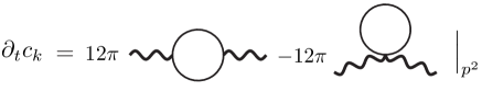
Figure 1: Diagrammatic representation of the flow equation of the $c$–function as given in equation (41).

$$\partial_{t}c_{k}=\left.12\pi\,\mbox{Tr}\,\tilde{\partial}_{t}\left\{G_{k}\frac{\delta^{3}\Gamma_{k}^{WZ}}{\delta\tau\delta\varphi\delta\varphi}G_{k}\frac{\delta^{3}\Gamma_{k}^{WZ}}{\delta\tau\delta\varphi\delta\varphi}\right\}\right|_{p^{2}}-12\pi\left.\mbox{Tr}\,\tilde{\partial}_{t}\left\{G_{k}\frac{\delta^{4}\Gamma_{k}^{WZ}}{\delta\tau\delta\tau\delta\varphi\delta\varphi}\right\}\right|_{p^{2}}\,,$$ (41)

where $G_{k}\equiv\left(\Gamma_{k}^{\left(2,0\right)}+R_{k}\right)^{-1}$ and $\tilde{\partial}_{t}\equiv\partial_{t}R_{k}\frac{\partial}{\partial R_{k}}$ (for more details see [9]). This is the explicit flow equation for the $c$–function and it can be represented as in Figure 1. The non–trivial running is due to the interaction vertices between the matter fields (which run in the loop) and the dilaton.

5.2 Recovering the consistency conditions

We are now ready to combine the flow equation for the $c$–function (41) with the form of the derivative expansion of the running Wess–Zumino action we found in Section 3.

Since the vertices in the two diagrams of Figure 1 are matter–dilaton vertices, only the potential will contribute. This is a very important fact and will lead to a very simple form for the flow of the $c$–function. The first diagram of Figure 1, representing the first trace in equation (41), will involve the three point vertex stemming from the monomial $\tau\beta^{i}{\cal O}_{i}$, since all other higher order terms in the beta functions will not contribute once the dilaton is set to zero in the vertex. In this diagram the $p^{2}$ dependence is entirely due to one of the $G_{k}$ which is evaluated at $(q+p)^{2}$. The second diagram, representing the second trace in equation (41), will instead involve a vertex derived from $\tau^{2}\beta_{j}\partial_{j}\beta_{i}{\cal O}_{i}$. This however does not contribute to the running of the $c$–function since there are no derivatives acting on the dilaton producing $p^{2}$ contributions (remember that our deformations are primaries), and these cannot come from the $G_{k}$ since they are evaluated at $q^{2}$.

Thus we conclude that only the first diagram contributes: this implies that the final form of the flow equation is quadratic in the (dimensionless) beta functions. More precisely we find:

$$\partial_{t}c_{k}=24\pi\chi_{ij}\beta^{i}\beta^{j}\,,$$ (42)

where the FRG’s explicit form for Zamolodchikov’s metric is:

$$\chi_{ij}=\frac{1}{24\pi}\int\frac{d^{2}q}{(2\pi)^{2}}\tilde{\partial}_{t}\left\{G_{k}(q^{2})G_{k}\left((q+p)^{2}\right)\right\}\mathcal{O}_{i}^{(2)}(q,q+p)\mathcal{O}_{j}^{(2)}(-q-p,-q)\,.$$ (43)

Here $\mathcal{O}_{i}^{(2)}(q_{1},q_{2})$ denotes the momentum space representation of the vertex $\frac{\delta^{2}\mathcal{O}_{i}}{\delta\varphi\delta\varphi}$. These last two relations are the main result of this paper. It is clear that the FRG flow equation for the $c$–function (42) is exactly the same as the Weyl consistency condition (35) derived within the LRG approach. This result thus shows the, at least formal, equivalence of these two RG approaches in the two dimensional case. The only, relevant, difference is that the FRG approach furnishes an explicit representation for both the beta functions, via equation (37), and for Zamolodchikov’s metric, via equation (43).

6 Conclusion and Outlook

In this paper we have clarified the connection between the functional (or exact) renormalisation group (FRG) and the local renormalisation group (LRG) in the two dimensional case, showing that these two major techniques used to obtain information on QFTs arbitrarily far away from criticality are compatible and interconnected.

The proof of this connection was based on a careful analysis of the form of the scale dependent Wess–Zumino action. We have seen in particular that it is not only sufficient to identify the correct terms which reproduce the conformal anomaly at the fixed point: it is also important to constrain the form of the possible $\beta$–terms, which are generated along the flow and die out at its endpoints. These $\beta$–terms, called this way since they are proportional to beta functions, can be mapped into corresponding terms found in the LRG. In the latter framework, these terms simply arise as additional couplings due to the introduction of spacetime dependent sources. They are then connected to beta functions with the help of the Wess–Zumino consistency conditions. In this way, the consistency conditions imposed by Weyl symmetry are able to constrain the possible forms of the beta functions of the theory, and thus they provide information on its RG flow. As we already remarked, the physical idea lying behind this fact is that the sources used in the LRG act effectively like running couplings, whose RG scale has become spacetime dependent. This means that the scale transformations get promoted to Weyl transformations, which automatically satisfy Wess–Zumino consistency conditions due to the structure of the Weyl group.

However, our analysis has shown that the constraints on the form of the running Wess–Zumino action are fairly general, and in fact they can be used directly into the FRG to get the same results. In particular, one can show in general that the beta function of $c$ must be quadratic in the beta functions of the primary deformation couplings, a result usually obtained with the LRG. If the two points of view are put together, then the FRG gives a constructive way to compute the Zamolodchikov–Osborn metric $\chi_{ij}$ for specific field contents.

One important remark should be made, and regards the proper form of the $c$–function. In the LRG, the proper $c$–function is not simply the running central charge, or anomaly coefficient $\mathcal{C}_{k}$, but is instead $\mathcal{C}_{k}+\omega_{i}\beta^{i}$. However, as we saw form the general analysis in Section 3, this appears as the coefficient of the $\partial_{\mu}\tau\partial^{\mu}\tau$ term off–criticality, and at the FRG level it is quite indifferent how we choose to represent this coefficient: all we really need is to identify the proper monomial and then check its running. Now in two dimensions, if we project the running on a flat background, that choice is essentially unique, so we can pick that as our candidate $c$–function. In higher dimension such as $d=4$ this choice will in general be non–unique, so one must be more careful, but the same remark applies.

Our analysis can naturally be extended to $d=4$ or higher dimensions, with the proviso just made. This would be a particularly nice application since little is known in this case about the behaviour of the flow of the central charge far away from a conformal phase. We plan to explore these issues in a future work.

References

- [1] A. B. Zamolodchikov, JETP Lett. 43 (1986) 730 [Pisma Zh. Eksp. Teor. Fiz. 43 (1986) 565].
- [2] I. Jack and H. Osborn, Nucl. Phys. B 343 (1990) 647.
- [3] H. Osborn, Nucl. Phys. B 363 (1991) 486.
- [4] I. Jack and H. Osborn, Nucl. Phys. B 883 (2014) 425 [arXiv:1312.0428 [hep-th]].
- [5] Z. Komargodski and A. Schwimmer, JHEP 1112, 099 (2011) [arXiv:1107.3987 [hep-th]].
- [6] Z. Komargodski, JHEP 1207, 069 (2012) [arXiv:1112.4538 [hep-th]].
- [7] M. A. Luty, J. Polchinski and R. Rattazzi, JHEP 1301, 152 (2013) [arXiv:1204.5221 [hep-th]].
- [8] J. Berges, N. Tetradis and C. Wetterich, Phys. Rept. bf 363 (2002) 223 [hep-ph/0005122].
- [9] A. Codello, G. D’Odorico and C. Pagani, JHEP 1407 (2014) 040 [arXiv:1312.7097 [hep-th]].
- [10] M. J. Duff, Class. Quant. Grav. 11 (1994) 1387 [hep-th/9308075].
- [11] E. Mottola, J. Math. Phys. 36 (1995) 2470 [hep-th/9502109].
- [12] A. Codello, G. D’Odorico, C. Pagani and R. Percacci, Class.Quant. Grav. 30 (2013) 115015 [arXiv:1210.3284 [hep-th]].
- [13] C. Pagani and R. Percacci, Class. Quant. Grav. 31 (2014) 115005.
- [14] A. Codello and G. D’Odorico, arXiv:1412.6837 [gr-qc].
- [15] F. Baume, B. Keren-Zur, R. Rattazzi and L. Vitale, JHEP 1408 (2014) 152 [arXiv:1401.5983 [hep-th]].
- [16] B. Grinstein, A. Stergiou and D. Stone, JHEP 1311 (2013) 195 [arXiv:1308.1096 [hep-th]].
- [17] D. Friedan and A. Konechny, J. Phys. A 43 (2010) 215401 [arXiv:0910.3109 [hep-th]].
- [18] J. Wess and B. Zumino, Phys. Lett. B 37 (1971) 95.
- [19] D. Becker and M. Reuter, arXiv:1412.0468 [hep-th].
- [20] C. Wetterich, Phys. Lett. B 301 (1993) 90; T. R. Morris, Int. J. Mod. Phys. A 9 (1994) 2411, hep-ph/9308265.