The Power of Randomization
Distributed Submodular Maximization on Massive Datasets

Abstract

A wide variety of problems in machine learning, including exemplar clustering, document summarization, and sensor placement, can be cast as constrained submodular maximization problems. Unfortunately, the resulting submodular optimization problems are often too large to be solved on a single machine. We develop a simple distributed algorithm that is embarrassingly parallel and it achieves provable, constant factor, worst-case approximation guarantees. In our experiments, we demonstrate its efficiency in large problems with different kinds of constraints with objective values always close to what is achievable in the centralized setting.

1 Introduction

A set function $f:2^{V}\rightarrow{\mathbb{R}}_{\geq 0}$ on a ground set $V$ is submodular if $f(A)+f(B)\geq f(A\cap B)+f(A\cup B)$ for any two sets $A,B\subseteq V$. Several problems of interest can be modeled as maximizing a submodular objective function subject to certain constraints:

$$\max f(A)\text{ subject to }A\in\mathcal{C},$$

where $\mathcal{C}\subseteq 2^{V}$ is the family of feasible solutions. Indeed, the general meta-problem of optimizing a constrained submodular function captures a wide variety of problems in machine learning applications, including exemplar clustering, document summarization, sensor placement, image segmentation, maximum entropy sampling, and feature selection problems.

At the same time, in many of these applications, the amount of data that is collected is quite large and it is growing at a very fast pace. For example, the wide deployment of sensors has led to the collection of large amounts of measurements of the physical world. Similarly, medical data and human activity data are being captured and stored at an ever increasing rate and level of detail. This data is often high-dimensional and complex, and it needs to be stored and processed in a distributed fashion.

In these settings, it is apparent that the classical algorithmic approaches are no longer suitable and new algorithmic insights are needed in order to cope with these challenges. The algorithmic challenges stem from the following competing demands imposed by huge datasets: the computations need to process the data that is distributed across several machines using a minimal amount of communication and synchronization across the machines, and at the same time deliver solutions that are competitive with the centralized solution on the entire dataset.

The main question driving the current work is whether these competing goals can be reconciled. More precisely, can we deliver very good approximate solutions with minimal communication overhead? Perhaps surprisingly, the answer is yes; there is a very simple distributed greedy algorithm that is embarrassingly parallel and it achieves provable, constant factor, worst-case approximation guarantees. Our algorithm can be easily implemented in a parallel model of computation such as MapReduce [2].

1.1 Background and Related Work

In the MapReduce model, there are $m$ independent machines. Each of the machines has a limited amount of memory available. In our setting, we assume that the data is much larger than any single machine’s memory and so must be distributed across all of the machines. At a high level, a MapReduce computation proceeds in several rounds. In a given round, the data is shuffled among the machines. After the data is distributed, each of the machines performs some computation on the data that is available to it. The output of these computations is either returned as the final result or becomes the input to the next MapReduce round. We emphasize that the machines can only communicate and exchange data during the shuffle phase.

In order to put our contributions in context, we briefly discuss two distributed greedy algorithms that achieve complementary trade-offs in terms of approximation guarantees and communication overhead.

Mirzasoleiman et al. [10] give a distributed algorithm, called GreeDi, for maximizing a monotone submodular function subject to a cardinality constraint. The GreeDi algorithm partitions the data arbitrarily on the machines and on each machine it runs the classical Greedy algorithm to select a feasible subset of the items on that machine. The Greedy solutions on these machines are then placed on a single machine and the Greedy algorithm is used once more to select the final solution. The GreeDi algorithm is very simple and embarrassingly parallel, but its worst-case approximation guarantee is $1/\Theta\left(\min\left\{\sqrt{k},m\right\}\right)$, where $m$ is the number of machines and $k$ is the cardinality constraint. Despite this, Mirzasoleiman et al. show that the GreeDi algorithm achieves very good approximations for datasets with geometric structure.

Kumar et al. [8] give distributed algorithms for maximizing a monotone submodular function subject to a cardinality or more generally, a matroid constraint. Their algorithm combines the Threshold Greedy algorithm of [4] with a sample and prune strategy. In each round, the algorithm samples a small subset of the elements that fit on a single machine and runs the Threshold Greedy algorithm on the sample in order to obtain a feasible solution. This solution is then used to prune some of the elements in the dataset and reduce the size of the ground set. The Sample&Prune algorithms achieve constant factor approximation guarantees but they incur a higher communication overhead. For a cardinality constraint, the number of rounds is a constant but for more general constraints such as a matroid constraint, the number of rounds is $\Theta(\log{\Delta})$, where $\Delta$ is the maximum increase in the objective due to a single element. The maximum increase $\Delta$ can be much larger than even the number of elements in the entire dataset, which makes the approach infeasible for massive datasets.

On the negative side, Indyk et al. [5] studied coreset approaches to develop distributed algorithms for finding representative and yet diverse subsets in large collections. While succeeding in several measures, they also showed that their approach provably does not work for $k$-coverage, which is a special case of submodular maximization with a cardinality constraint.

1.2 Our Contribution

In this paper, we show that we can achieve both the communication efficiency of the GreeDi algorithm and a provable, constant factor, approximation guarantee. Our algorithm is in fact the GreeDi algorithm with a very simple and crucial modification: instead of partitioning the data arbitrarily on the machines, we randomly partition the dataset. Our analysis may perhaps provide some theoretical justification for the very good empirical performance of the GreeDi algorithm that was established previously in the extensive experiments of [10]. It also suggests the approach can deliver good performance in much wider settings than originally envisioned.

The GreeDi algorithm was originally studied in the special case of monotone submodular maximization under a cardinality constraint. In contrast, our analysis holds for any hereditary constraint. Specifically, we show that our randomized variant of the GreeDi algorithm achieves a constant factor approximation for any hereditary, constrained problem for which the classical (centralized) Greedy algorithm achieves a constant factor approximation. This is the case not only for cardinality constraints, but also for matroid constraints, knapsack constraints, and $p$-system constraints [6], which generalize the intersection of $p$ matroid constraints. Table 4 gives the approximation ratio $\alpha$ obtained by the greedy algorithm on a variety of problems, and the corresponding constant factor obtained by our randomized GreeDi algorithm.

Constraint	$\alpha$	monotone approx. $\left(\frac{\alpha}{2}\right)$	non-monotone approx. $\left(\frac{\alpha}{4+2\alpha}\right)$
cardinality	$1-\frac{1}{e}\approx 0.632$	$\approx 0.316$	$\approx$ 0.12
matroid	$\frac{1}{2}$	$\frac{1}{4}$	$\frac{1}{10}$
knapsack	$\approx 0.35$	$\approx 0.17$	$\approx 0.074$
$p$-system	$\frac{1}{p+1}$	$\frac{1}{2(p+1)}$	$\frac{1}{2+4(p+1)}$

Table 1: New approximation results for randomized GreeDi for constrained monotone and non-monotone submodular maximization

Additionally, we show that if the greedy algorithm satisfies a slightly stronger technical condition, then our approach gives a constant factor approximation for constrained non-monotone submodular maximization. This is indeed the case for all of the aforementioned specific classes of problems. The resulting approximation ratios for non-monotone maximization problems are given in the last column of Table 4.

1.3 Preliminaries

MapReduce Model. In a MapReduce computation, the data is represented as $\left<\mathrm{key},\mathrm{value}\right>$ pairs and it is distributed across $m$ machines. The computation proceeds in rounds. In a given, the data is processed in parallel on each of the machines by map tasks that output $\left<\mathrm{key},\mathrm{value}\right>$ pairs. These pairs are then shuffled by reduce tasks; each reduce task processes all the $\left<\mathrm{key},\mathrm{value}\right>$ pairs with a given key. The output of the reduce tasks either becomes the final output of the MapReduce computation or it serves as the input of the next MapReduce round.

Submodularity. As noted in the introduction, a set function $f:2^{V}\to{\mathbb{R}}_{\geq 0}$ is submodular if, for all sets $A,B\subseteq V$,

$$f(A)+f(B)\geq f(A\cup B)+f(A\cap B).$$

A useful alternative characterization of submodularity can be formulated in terms of diminishing marginal gains. Specifically, $f$ is submodular if and only if:

$$f(A\cup\left\{e\right\})-f(A)\geq f(B\cup\left\{e\right\})-f(B)$$

for all $A\subseteq B\subseteq V$ and $e\notin B$.

The Lovász extension $f^{-}:[0,1]^{V}\to{\mathbb{R}}_{\geq 0}$ of a submodular function $f$ is given by:

$$f^{-}({\mathbf{x}})=\operatorname*{\mathbb{E}}_{\theta\in\mathcal{U}(0,1)}[f(\{i:x_{i}\geq\theta\})].$$

For any submodular function $f$, the Lovász extension $f^{-}$ satisfies the following properties: (1) $f^{-}(\mathbf{1}_{S})=f(S)$ for all $S\subseteq V$, (2) $f^{-}$ is convex, and (3) $f^{-}(c\cdot{\mathbf{x}})\geq c\cdot f^{-}({\mathbf{x}})$ for any $c\in[0,1]$. These three properties immediately give the following simple lemma:

Lemma 1.

Let $S$ be a random set, and suppose that $\operatorname*{\mathbb{E}}[\mathbf{1}_{S}]=c\cdot{\mathbf{p}}$ (for $c\in[0,1]$). Then, $\operatorname*{\mathbb{E}}[f(S)]\geq c\cdot f^{-}({\mathbf{p}})$.

Proof.

We have:

$$\operatorname*{\mathbb{E}}[f(S)]=\operatorname*{\mathbb{E}}[f^{-}(\mathbf{1}_{S})]\geq f^{-}(\operatorname*{\mathbb{E}}[\mathbf{1}_{S}])=f^{-}(c\cdot{\mathbf{p}})\geq c\cdot f^{-}({\mathbf{p}}),$$

where the first equality follows from property (1), the first inequality from property (2), and the final inequality from property (3). ∎

Hereditary Constraints. Our results hold quite generally for any problem which can be formulated in terms of a hereditary constraint. Formally, we consider the problem

$$\max\{f(S):S\subseteq V,S\in\mathcal{I}\},$$ (1)

where $f:2^{V}\to{\mathbb{R}}_{\geq 0}$ is a submodular function and $\mathcal{I}\subseteq 2^{V}$ is a family of feasible subsets of $V$. We require that $\mathcal{I}$ be hereditary in the sense that if some set is in $\mathcal{I}$, then so are all of its subsets. Examples of common hereditary families include cardinality constraints ($\mathcal{I}=\{A\subseteq V:|A|\leq k\}$), matroid constraints ($\mathcal{I}$ corresponds to the collection independent sets of the matroid), knapsack constraints ($\mathcal{I}=\{A\subseteq V:\sum_{i\in A}w_{i}\leq b\}$), as well as arbitrary combinations of such constraints. Given some constraint $\mathcal{I}\subseteq 2^{V}$, we shall also consider restricted instances in which we are presented only with a subset $V^{\prime}\subseteq V$, and must find a set $S\subseteq V^{\prime}$ with $S\in\mathcal{I}$ that maximizes $f$. We say that an algorithm is an $\alpha$-approximation for maximizing a submodular function subject to a hereditary constraint $\mathcal{I}$ if, for any submodular function $f:2^{V}\to{\mathbb{R}}_{\geq 0}$ and any subset $V^{\prime}\subseteq V$ the algorithm produces a solution $S\subseteq V^{\prime}$ with $S\in\mathcal{I}$, satisfying $f(S)\geq\alpha\cdot f(\mathrm{OPT})$, where $\mathrm{OPT}\in\mathcal{I}$ is any feasible subset of $V^{\prime}$.

2 The Standard Greedy Algorithm

Algorithm 1 The standard greedy algorithm Greedy

  $S\leftarrow\emptyset$

  loop

     Let $C=\{e\in V\setminus S:S\cup\left\{e\right\}\in\mathcal{I}\}$

     Let $e=\arg\max_{e\in C}\{f(S\cup\left\{e\right\})-f(S)\}$

     if $C=\emptyset$ or $f(S\cup\left\{e\right\})-f(S)<0$ then

        return $S$

     end if

  end loop

Algorithm 2 The distributed algorithm RandGreeDi

  for $e\in V$ do

     Assign $e$ to a machine $i$ chosen uniformly at random

  end for

  Let $V_{i}$ be the elements assigned to machine $i$

  Run $\textsc{Greedy}(V_{i})$ on each machine $i$ to obtain $S_{i}$

  Place $S=\bigcup_{i}S_{i}$ on machine $1$

  Run $\textsc{Alg}(S)$ on machine $1$ to obtain $T$

  Let $S^{\prime}=\arg\max_{i}\{f(S_{i})\}$

  return $\arg\max\{f(T),f(S^{\prime})\}$

Before describing our general algorithm, let us recall the standard greedy algorithm, Greedy, shown in Algorithm 1. The algorithm takes as input $\langle V,\mathcal{I},f\rangle$, where $V$ is a set of elements, $\mathcal{I}\subseteq 2^{V}$ is a hereditary constraint, represented as a membership oracle for $\mathcal{I}$, and $f:2^{V}\to{\mathbb{R}}_{\geq 0}$ is a non-negative submodular function, represented as a value oracle. Given $\langle V,\mathcal{I},f\rangle$, Greedy iteratively constructs a solution $S\in\mathcal{I}$ by choosing at each step the element maximizing the marginal increase of $f$. For some $A\subseteq V$, we let $\textsc{Greedy}(A)$ denote the set $S\in\mathcal{I}$ produced by the greedy algorithm that considers only elements from $A$.

The greedy algorithm satisfies the following property:

Lemma 2.

Let $A\subseteq V$ and $B\subseteq V$ be two disjoint subsets of $V$. Suppose that, for each element $e\in B$, we have $\textsc{Greedy}(A\cup\left\{e\right\})=\textsc{Greedy}(A)$. Then $\textsc{Greedy}(A\cup B)=\textsc{Greedy}(A)$.

Proof.

Suppose for contradiction that $\textsc{Greedy}(A\cup B)\neq\textsc{Greedy}(A)$. We first note that, if $\textsc{Greedy}(A\cup B)\subseteq A$, then $\textsc{Greedy}(A\cup B)=\textsc{Greedy}(A)$; this follows from the fact that each iteration of the Greedy algorithm chooses the element with the highest marginal value whose addition to the current solution maintains feasibility for $\mathcal{I}$. Therefore, if $\textsc{Greedy}(A\cup B)\neq\textsc{Greedy}(A)$, the former solution contains an element of $B$. Let $e$ be the first element of $B$ that is selected by Greedy on the input $A\cup B$. Then Greedy will also select $e$ on the input $A\cup\left\{e\right\}$, which contradicts the fact that $\textsc{Greedy}(A\cup\left\{e\right\})=\textsc{Greedy}(A)$. ∎

3 A Randomized, Distributed Greedy Algorithm for Monotone Submodular Maximization

Algorithm. We now describe our general, randomized distributed algorithm, RandGreeDi, shown in Algorithm 2. Suppose we have $m$ machines. Our algorithm runs in two rounds. In the first round, we randomly distribute the elements of the ground set $V$ to the machines, assigning each element to a machine chosen independently and uniformly at random. On each machine $i$, we execute $\textsc{Greedy}(V_{i})$ to select a feasible subset $S_{i}$ of the elements on that machine. In the second round, we place all of these selected subsets on a single machine, and run some algorithm Alg on this machine in order to select a final solution $T$. We return whichever is better: the final solution $T$ or the best solution amongst all the $S_{i}$ from the first phase.

Analysis. We devote the rest of this section to the analysis of the RandGreeDi algorithm. Fix $\langle V,\mathcal{I},f\rangle$, where $\mathcal{I}\subseteq 2^{V}$ is a hereditary constraint, and $f:2^{V}\to{\mathbb{R}}_{\geq 0}$ is any non-negative, monotone submodular function. Suppose that Greedy is an $\alpha$-approximation and Alg is a $\beta$-approximation for the associated constrained monotone submodular maximization problem of the form (1). Let $n=|V|$ and suppose that $\mathrm{OPT}=\arg\max_{A\in\mathcal{I}}f(A)$ is a feasible set maximizing $f$.

Let $\mathcal{V}(1/m)$ denote the distribution over random subsets of $V$ where each element is included independently with probability $1/m$. Let ${\mathbf{p}}\in[0,1]^{n}$ be the following vector. For each element $e\in V$, we have

$$p_{e}=\begin{cases}\underset{A\sim\mathcal{V}(1/m)}{\Pr}[e\in\textsc{Greedy}(A\cup\left\{e\right\})]&\text{if $e\in\mathrm{OPT}$}\\ 0&\text{otherwise}\end{cases}$$

Our main theorem follows from the next two lemmas, which characterize the quality of the best solution from the first round and that of the solution from the second round, respectively. Recall that $f^{-}$ is the Lovász extension of $f$.

Lemma 3.

For each machine $i$, $\operatorname*{\mathbb{E}}[f(S_{i})]\geq\alpha\cdot f^{-}\left({\mathbf{1}}_{\mathrm{OPT}}-{\mathbf{p}}\right).$

Proof.

Consider machine $i$. Let $V_{i}$ denote the set of elements assigned to machine $i$ in the first round. Let $O_{i}=\left\{e\in\mathrm{OPT}\colon e\notin\textsc{Greedy}(V_{i}\cup\left\{e\right\})\right\}$. We make the following key observations.

We apply Lemma 2 with $A=V_{i}$ and $B=O_{i}\setminus V_{i}$ to obtain that $\textsc{Greedy}(V_{i})=\textsc{Greedy}(V_{i}\cup O_{i})=S_{i}$. Since $\mathrm{OPT}\in\mathcal{I}$ and $\mathcal{I}$ is hereditary, we must have $O_{i}\in\mathcal{I}$ as well. Since Greedy is an $\alpha$-approximation, it follows that

$$f(S_{i})\geq\alpha\cdot f(O_{i}).$$

Since the distribution of $V_{i}$ is the same as $\mathcal{V}(1/m)$, for each element $e\in\mathrm{OPT}$, we have

$$\Pr[e\in O_{i}] =1-\Pr[e\notin O_{i}]=1-p_{e}$$

$$\operatorname*{\mathbb{E}}[\mathbf{1}_{O_{i}}] =\mathbf{1}_{\mathrm{OPT}}-{\mathbf{p}}.$$

By combining these observations with Lemma 1, we obtain

$$\operatorname*{\mathbb{E}}[f(S_{i})]\geq\alpha\cdot\operatorname*{\mathbb{E}}[f(O_{i})]\geq\alpha\cdot f^{-}\left({\mathbf{1}}_{\mathrm{OPT}}-{\mathbf{p}}\right).$$

∎

Lemma 4.

$\operatorname*{\mathbb{E}}[f(\textsc{Alg}(S))]\geq\beta\cdot f^{-}({\mathbf{p}}).$

Proof.

Recall that $S=\bigcup_{i}\textsc{Greedy}(V_{i})$. Since $\mathrm{OPT}\in\mathcal{I}$ and $\mathcal{I}$ is hereditary, $S\cap\mathrm{OPT}\in\mathcal{I}$. Since Alg is a $\beta$-approximation, we have

$$f(\textsc{Alg}(S))\geq\beta\cdotp f(S\cap\mathrm{OPT}).$$ (2)

Consider an element $e\in\mathrm{OPT}$. For each machine $i$, we have

$$\Pr[e\in S\;|\;\text{$e$ is assigned to machine $i$}] =\Pr[e\in\textsc{Greedy}(V_{i})\;|\;e\in V_{i}]$$

$$=\Pr_{A\sim\mathcal{V}(1/m)}[e\in\textsc{Greedy}(A)\;|\;e\in A]$$

$$=\Pr_{B\sim\mathcal{V}(1/m)}[e\in\textsc{Greedy}(B\cup\left\{e\right\})]$$

$$=p_{e}.$$

The first equality follows from the fact that $e$ is included in $S$ if and only if it is included in $\textsc{Greedy}(V_{i})$. The second equality follows from the fact that the distribution of $V_{i}$ is identical to $\mathcal{V}(1/m)$. The third equality follows from the fact that the distribution of $A\sim\mathcal{V}(1/m)$ conditioned on $e\in A$ is identical to the distribution of $B\cup\{e\}$ where $B\sim\mathcal{V}(1/m)$. Therefore

$$\Pr[e\in S\cap\mathrm{OPT}] =p_{e}$$

$$\operatorname*{\mathbb{E}}[\mathbf{1}_{S\cap\mathrm{OPT}}] ={\mathbf{p}}.$$ (3)

By combining (2), (3), and Lemma 1, we obtain

$$\operatorname*{\mathbb{E}}[f(\textsc{Alg}(S))]\geq\beta\cdotp\operatorname*{\mathbb{E}}[f(S\cap\mathrm{OPT})]\geq\beta\cdot f^{-}({\mathbf{p}}).$$

∎

Combining Lemma 4 and Lemma 3 gives us our main theorem.

Theorem 5.

Suppose that Greedy is an $\alpha$-approximation algorithm and Alg is a $\beta$-approximation algorithm for maximizing a monotone submodular function subject to a hereditary constraint $\mathcal{I}$. Then RandGreeDi is (in expectation) an $\frac{\alpha\beta}{\alpha+\beta}$-approximation algorithm for the same problem.

Proof.

Let $S_{i}=\textsc{Greedy}(V_{i})$, $S=\bigcup_{i}S_{i}$ be the set of elements on the last machine, and $T=\textsc{Alg}(S)$ be the solution produced on the last machine. Then, the output $D$ produced by RandGreeDi satisfies $f(D)\geq\max_{i}(f(S_{i}))$ and $f(D)\geq f(T)$. Thus, from Lemmas 3 and 4 we have:

$$\operatorname*{\mathbb{E}}[f(D)] \geq\alpha\cdot f^{-}(\mathbf{1}_{\mathrm{OPT}}-{\mathbf{p}})$$ (4)

$$\operatorname*{\mathbb{E}}[f(D)] \geq\beta\cdot f^{-}({\mathbf{p}}).$$ (5)

By combining (4) and (5), we obtain

$$\left(\beta+\alpha\right)\operatorname*{\mathbb{E}}[f(D)] \geq\alpha\beta\big{(}f^{-}({\mathbf{p}})+f^{-}(\mathbf{1}_{\mathrm{OPT}}-{\mathbf{p}})\big{)}$$

$$\geq\alpha\beta\cdot f^{-}(\mathbf{1}_{\mathrm{OPT}})$$

$$=\alpha\beta\cdot f(\mathrm{OPT}).$$

In the second inequality, we have used the fact that $f^{-}$ is convex and $f^{-}(c\cdotp{\mathbf{x}})\geq cf^{-}({\mathbf{x}})$ for any constant $c\in[0,1]$. ∎

If we use the standard greedy algorithm for Alg, we obtain the following simplified corollary of Theorem 5.

Corollary 6.

Suppose that Greedy is an $\alpha$-approximation algorithm for maximizing a monotone submodular function, and use Greedy as the algorithm Alg in RandGreeDi. Then, the resulting algorithm is (in expectation) an $\frac{\alpha}{2}$-approximation algorithm for the same problem.

4 Non-Monotone Submodular Functions

We consider the problem of maximizing a non-monotone submodular function subject to a hereditary constraint. Our approach is a slight modification of the randomized, distributed greedy algorithm described in Section 3, and it builds on the work of [4]. Again, we show how to combine the standard Greedy algorithm, together with any algorithm Alg for the non-monotone case in order to obtain a randomized, distributed algorithm for the non-monotone submodular maximization.

Algorithm. Our modified algorithm, NMRandGreeDi, works as follows. As in the monotone case, in the first round we distribute the elements of $V$ uniformly at random amongst the $m$ machines. Then, we run the standard greedy algorithm twice to obtain two disjoint solutions $S_{i}^{1}$ and $S_{i}^{2}$ on each machine. Specifically, each machine first runs Greedy on $V_{i}$ to obtain a solution $S_{i}^{1}$, then runs Greedy on $V_{i}\setminus S_{i}^{1}$ to obtain a disjoint solution $S_{i}^{2}$. In the second round, both of these solutions are sent to a single machine, which runs Alg on $S=\bigcup_{i}(S_{i}^{1}\cup S_{i}^{2})$ to produce a solution $T$. The best solution amongst $T$ and all of the solutions $S_{i}^{1}$ and $S_{i}^{2}$ is then returned.

Analysis. We devote the rest of this section to the analysis of the algorithm. In the following, we assume that we are working with an instance $\langle V,\mathcal{I},f\rangle$ of non-negative, non-monotone submodular maximization for which the Greedy algorithm has the following property:

$$\text{For all $S\in\mathcal{I}$:}\qquad f(\textsc{Greedy}(V))\geq\alpha\cdot f(\textsc{Greedy}(V)\cup S) \mathrm{GP}$$ ()

The standard analysis of the Greedy algorithm shows that ($\mathrm{GP}$) is satisfied with constant $\alpha$ for hereditary constraints such as matroids, knapsacks, and $p$-systems (see Table 4).

The analysis is similar to the approach from the previous section. We define $\mathcal{V}(1/m)$ as before. We modify the definition of the vector ${\mathbf{p}}$ as follows. For each element $e\in V$, we have

$$p_{e}=\begin{cases}\underset{A\sim\mathcal{V}(1/m)}{\Pr}\Big{[}e\in\textsc{Greedy}(A\cup\{e\})\textbf{ or }&\\ \qquad\qquad\;e\in\textsc{Greedy}((A\cup\{e\})\setminus\textsc{Greedy}(A\cup\{e\}))\Big{]}&\text{if $e\in\mathrm{OPT}$}\\ 0&\text{otherwise}\end{cases}$$

We now derive analogues of Lemmas 3 and 4.

Lemma 7.

Suppose that Greedy satisfies ($\mathrm{GP}$). For each machine $i$,

$$\operatorname*{\mathbb{E}}\left[f(S^{1}_{i})+f(S^{2}_{i})\right]\geq\alpha\cdotp f^{-}({\mathbf{1}}_{\mathrm{OPT}}-{\mathbf{p}}),$$

and therefore

$$\operatorname*{\mathbb{E}}\left[\max\left\{f(S^{1}_{i}),f(S^{2}_{i})\right\}\right]\geq\frac{\alpha}{2}\cdotp f^{-}({\mathbf{1}}_{\mathrm{OPT}}-{\mathbf{p}}).$$

Proof.

Consider machine $i$ and let $V_{i}$ be the set of elements assigned to machine $i$ in the first round. Let

$$O_{i}=\{e\in\mathrm{OPT}\colon e \notin\textsc{Greedy}(V_{i}\cup\left\{e\right\})\textbf{ and }$$

$$e \notin\textsc{Greedy}((V_{i}\cup\left\{e\right\})\setminus\textsc{Greedy}(V_{i}\cup\left\{e\right\}))\}$$

Note that, since $\mathrm{OPT}\in\mathcal{I}$ and $\mathcal{I}$ is hereditary, we have $O_{i}\in\mathcal{I}$.

It follows from Lemma 2 that

$$S^{1}_{i} =\textsc{Greedy}(V_{i})=\textsc{Greedy}(V_{i}\cup O_{i}),$$ (6)

$$S^{2}_{i} =\textsc{Greedy}(V_{i}\setminus S^{1}_{i})=\textsc{Greedy}((V_{i}\setminus S^{1}_{i})\cup O_{i}).$$ (7)

By combining the equations above with the greedy property ($\mathrm{GP}$), we obtain

$$f(S^{1}_{i}) \overset{(\ref{eq:rejected1})}{=}f(\textsc{Greedy}(V_{i}\cup O_{i}))$$

$$\overset{(\ref{eq:greedy-strong-property})}{\geq}\alpha\cdotp f(\textsc{Greedy}(V_{i}\cup O_{i})\cup O_{i})$$

$$\overset{(\ref{eq:rejected1})}{=}\alpha\cdotp f(S^{1}_{i}\cup O_{i}),$$ (8)

$$f(S^{2}_{i}) \overset{(\ref{eq:rejected2})}{=}f(\textsc{Greedy}((V_{i}\setminus S^{1}_{i})\cup O_{i}))$$

$$\overset{(\ref{eq:greedy-strong-property})}{\geq}\alpha\cdotp f(\textsc{Greedy}((V_{i}\setminus S^{1}_{i})\cup O_{i})\cup O_{i})$$

$$\overset{(\ref{eq:rejected2})}{=}\alpha\cdotp f(S^{2}_{i}\cup O_{i}).$$ (9)

Now we observe that

$$f(S^{1}_{i}\cup O_{i})+f(S^{2}_{i}\cup O_{i}) \geq f((S^{1}_{i}\cup O_{i})\cap(S^{2}_{i}\cup O_{i}))+f(S^{1}_{i}\cup S^{2}_{i}\cup O_{i}) f$$ ( is submodular)

$$=f(O_{i})+f(S^{1}_{i}\cup S^{2}_{i}\cup O_{i}) S^{1}_{i}\cap S^{2}_{i}=\emptyset$$ ()

$$\geq f(O_{i}). f$$ ( is non-negative) (10)

By combining (8), (9), and (10), we obtain

$$f(S^{1}_{i})+f(S^{2}_{i})\geq\alpha\cdotp f(O_{i}).$$ (11)

Since the distribution of $V_{i}$ is the same as $\mathcal{V}(1/m)$, for each element $e\in\mathrm{OPT}$, we have

$$\Pr[e\in O_{i}] =1-\Pr[e\notin O_{i}]=1-p_{e},$$

$$\operatorname*{\mathbb{E}}[\mathbf{1}_{O_{i}}] =\mathbf{1}_{\mathrm{OPT}}-{\mathbf{p}}.$$ (12)

By combining (11), (12), and Lemma 1, we obtain

$$\operatorname*{\mathbb{E}}[f(S^{1}_{i})+f(S^{2}_{i})] \geq\alpha\cdotp\operatorname*{\mathbb{E}}[f(O_{i})]$$ (By (11))

$$\geq\alpha\cdotp f^{-}(\mathbf{1}_{\mathrm{OPT}}-{\mathbf{p}}).$$ (By (12) and Lemma 1)

∎

Lemma 8.

$\operatorname*{\mathbb{E}}[f(\textsc{Alg}(S))]\geq\beta\cdot f^{-}({\mathbf{p}}).$

Proof.

Recall that $S^{1}_{i}=\textsc{Greedy}(V_{i})$, $S^{2}_{i}=\textsc{Greedy}(V_{i}\setminus S^{1}_{i})$, and $S=\bigcup_{i}(S^{1}_{i}\cup S^{2}_{i})$. Since $\mathrm{OPT}\in\mathcal{I}$ and $\mathcal{I}$ is hereditary, $S\cap\mathrm{OPT}\in\mathcal{I}$. Since Alg is a $\beta$-approximation, we have

$$f(\textsc{Alg}(S))\geq\beta\cdotp f(S\cap\mathrm{OPT}).$$ (13)

Consider an element $e\in\mathrm{OPT}$. For each machine $i$, we have

$$\Pr[e\in S\;|\;\text{$e$ is assigned to machine $i$}]$$

$$\quad=\Pr[e\in\textsc{Greedy}(V_{i})\textbf{ or }e\in\textsc{Greedy}(V_{i}\setminus\textsc{Greedy}(V_{i}))\;|\;e\in V_{i}]$$

$$\quad=\Pr_{A\sim\mathcal{V}(1/m)}[e\in\textsc{Greedy}(A)\textbf{ or }e\in\textsc{Greedy}(A\setminus\textsc{Greedy}(A))\;|\;e\in A]$$

$$\quad=\Pr_{B\sim\mathcal{V}(1/m)}[e\in\textsc{Greedy}(B\cup\left\{e\right\})\textbf{ or }e\in\textsc{Greedy}((B\cup\left\{e\right\})\setminus\textsc{Greedy}(B\cup\left\{e\right\}))]$$

$$\quad=p_{e}.$$

The first equality above follows from the fact that $e$ is included in $S$ iff $e$ is included in either $S_{i}^{1}$ or $S_{i}^{2}$. The second equality follows from the fact that the distribution of $V_{i}$ is the same as $\mathcal{V}(1/m)$. The third equality follows from the fact that the distribution of $A\sim\mathcal{V}(1/m)$ conditioned on $e\in A$ is identical to the distribution of $B\cup\{e\}$ where $B\sim\mathcal{V}(1/m)$. Therefore

$$\Pr[e\in S\cap\mathrm{OPT}] =p_{e},$$

$$\operatorname*{\mathbb{E}}[\mathbf{1}_{S\cap\mathrm{OPT}}] ={\mathbf{p}}.$$ (14)

By combining (13), (14), and Lemma 1, we obtain

$$\operatorname*{\mathbb{E}}[f(\textsc{Alg}(S))]\geq\beta\cdotp\operatorname*{\mathbb{E}}[f(S\cap\mathrm{OPT})]\geq\beta\cdot f^{-}({\mathbf{p}}).$$

∎

We can now combine Lemmas 8 and 7 to obtain our main result for non-monotone submodular maximization.

Theorem 9.

Consider the problem of maximizing a submodular function under some hereditary constraint $\mathcal{I}$, and suppose that Greedy satisfies ($\mathrm{GP}$) and Alg is a $\beta$-approximation algorithm for this problem. Then NMRandGreeDi is (in expectation) an $\frac{\alpha\beta}{\alpha+2\beta}$-approximation algorithm for the same problem.

Proof.

Let $S^{1}_{i}=\textsc{Greedy}(V_{i})$, $S^{2}_{i}=\textsc{Greedy}(V_{i}\setminus S^{1}_{i})$, and $S=\bigcup_{i}(S^{1}_{i}\cup S^{2}_{i})$ be the set of elements on the last machine, and $T=\textsc{Alg}(S)$ be the solution produced on the last machine. Then, the output $D$ produced by RandGreeDi satisfies $f(D)\geq\max_{i}\max\{f(S^{1}_{i}),f(S^{2}_{i})\}$ and $f(D)\geq f(T)$. Thus, from Lemmas 7 and 8 we have:

$$\operatorname*{\mathbb{E}}[f(D)] \geq\frac{\alpha}{2}\cdot f^{-}(\mathbf{1}_{\mathrm{OPT}}-{\mathbf{p}}),$$ (15)

$$\operatorname*{\mathbb{E}}[f(D)] \geq\beta\cdot f^{-}({\mathbf{p}}).$$ (16)

By combining (15) and (16), we obtain

$$\left(2\beta+\alpha\right)\operatorname*{\mathbb{E}}[f(D)] \geq\alpha\beta[f^{-}({\mathbf{p}})+f^{-}(\mathbf{1}_{\mathrm{OPT}}-{\mathbf{p}})]$$

$$\geq\alpha\beta\cdot f^{-}(\mathbf{1}_{\mathrm{OPT}})$$

$$=\alpha\beta\cdot f(\mathrm{OPT}).$$

In the second inequality, we have used the fact that $f^{-}$ is convex and $f^{-}(c\cdotp{\mathbf{x}})\geq cf^{-}({\mathbf{x}})$ for any constant $c\in[0,1]$. ∎

We remark that one can use the following approach on the last machine [4]. As in the first round, we run Greedy twice to obtain two solutions $T_{1}=\textsc{Greedy}(S)$ and $T_{2}=\textsc{Greedy}(S\setminus T_{1})$. Additionally, we select a subset $T_{3}\subseteq T_{1}$ using an unconstrained submodular maximization algorithm on $T_{1}$, such as the Double Greedy algorithm of [1], which is a $\frac{1}{2}$-approximation. The final solution $T$ is the best solution among $T_{1},T_{2},T_{3}$. If Greedy satisfies property $\mathrm{GP}$, then it follows from the analysis of [4] that the resulting solution $T$ satisfies $f(T)\geq\frac{\alpha}{2(1+\alpha)}\cdot f(\mathrm{OPT})$. This gives us the following corollary of Theorem 9:

Corollary 10.

Consider the problem of maximizing a submodular function subject to some hereditary constraint $\mathcal{I}$ and suppose that Greedy satisfies ($\mathrm{GP}$) for this problem. Let Alg be the algorithm described above that uses Greedy twice and Double Greedy. Then NMRandGreeDi achieves (in expectation) an $\frac{\alpha}{4+2\alpha}$-approximation for the same problem.

Proof.

By ($\mathrm{GP}$) and the approximation guarantee of the Double Greedy algorithm, we have:

$$f(T)\geq f(T_{1}) \geq\alpha\cdot f(T_{1}\cup\mathrm{OPT})$$ (17)

$$f(T)\geq f(T_{2}) \geq\alpha\cdot f(T_{2}\cup(\mathrm{OPT}\setminus T_{1}))$$ (18)

$$f(T)\geq f(T_{3}) \geq\frac{1}{2}f(T_{1}\cap\mathrm{OPT}).$$ (19)

Additionally, from [4, Lemma 2], we have:

$$f(T_{1}\cup\mathrm{OPT})+f(T_{2}\cup(\mathrm{OPT}\setminus T_{1}))+f(T_{1}\cap\mathrm{OPT})\geq f(\mathrm{OPT})$$

By combining the inequalities above, we obtain:

$$(1+\alpha)f(T)\geq\frac{\alpha}{2}\left(f(T_{1}\cup\mathrm{OPT})+f(T_{2}\cup(\mathrm{OPT}\setminus T_{1}))+f(T_{1}\cap\mathrm{OPT})\right)\geq\frac{\alpha}{2}f(\mathrm{OPT})$$

and hence $f(T)\geq\frac{\alpha}{2(1+\alpha)}\cdot f(\mathrm{OPT})$ as claimed. Setting $\beta=\frac{\alpha}{2(\alpha+1)}$ in Theorem 9, we obtain an approximation ratio of $\frac{\alpha}{4+2\alpha}$. ∎

5 Experiments

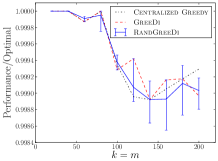
(a) Kosarak dataset

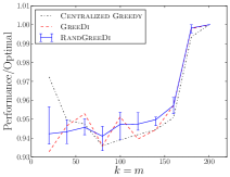
(b) accidents dataset

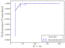
(c) 10K tiny images

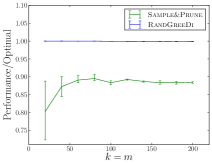
(d) Kosarak dataset

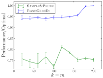
(e) accidents dataset

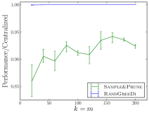
(f) 10K tiny images

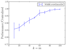
(g) synthetic diverse-yet-relevant instance ($n=10000$, $\lambda=n/k$)

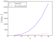
(h) synthetic hard instance for GreeDi

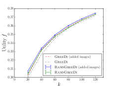
(i) 1M tiny images

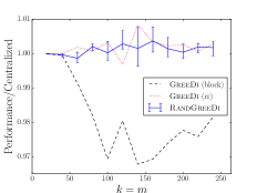
(j) matroid coverage $(n=900,r=5)$

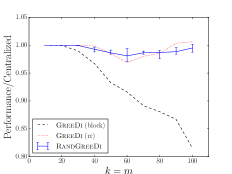
(k) matroid coverage $(n=100,r=100)$

Figure 1: Experimental Results

We experimentally evaluate and compare the following distributed algorithms for maximizing a monotone submodular function subject to a cardinality constraint: the RandGreeDi algorithm described in Section 3, the deterministic GreeDi algorithm of [10], and the Sample&Prune algorithm of [8]. We run these algorithms in several scenarios and we evaluate their performance relative to the centralized Greedy solution on the entire dataset.

Exemplar based clustering. Our experimental setup is similar to that of [10]. Our goal is to find a representative set of objects from a dataset by solving a $k$-medoid problem [7] that aims to minimize the sum of pairwise dissimilarities between the chosen objects and the entire dataset. Let $V$ denote the set of objects in the dataset and let $d:V\times V\rightarrow{\mathbb{R}}$ be a dissimilarity function; we assume that $d$ is symmetric, that is, $d(i,j)=d(j,i)$ for each pair $i,j$. Let $L:2^{V}\rightarrow{\mathbb{R}}$ be the function such that $L(A)={1\over\left|V\right|}\sum_{v\in V}\min_{a\in A}d(a,v)$ for each set $A\subseteq V$. We can turn the problem of minimizing $L$ into the problem of maximizing a monotone submodular function $f$ by introducing an auxiliary element $v_{0}$ and by defining $f(S)=L(\left\{v_{0}\right\})-L(S\cup\left\{v_{0}\right\})$ for each set $S\subseteq V$.

Tiny Images experiments: In our experiments, we used a subset of the Tiny Images dataset consisting of $32\times 32$ RGB images [12], each represented as $3,072$ dimensional vector. We subtracted from each vector the mean value and normalized the result, to obtain a collection of $3,072$-dimensional vectors of unit norm. We considered the distance function $d(x,y)=\|x-y\|^{2}$ for every pair $x,y$ of vectors. We used the zero vector as the auxiliary element $v_{0}$ in the definition of $f$.

In our smaller experiments, we used 10,000 tiny images, and compared the utility of each algorithm to that of the centralized greedy. The results are summarized in Figures 1(c) and 1(f).

In our large scale experiments, we used one million tiny images, and $m=100$ machines. In the first round of the distributed algorithm, each machine ran the Greedy algorithm to maximize a restricted objective function $f$, which is based on the average dissimilarity $L$ taken over only those images assigned to that machine. Similarly, in the second round, the final machine maximized an objective function $f$ based on the total dissimilarity of all those images it received . We also considered a variant similar to that described by [10], in which 10,000 additional random images from the original dataset were added to the final machine. The results are summarized in Figure 1(i).

Remark on the function evaluation. In decomposable cases such as exemplar clustering, the function is a sum of distances over all points in the dataset. By concentration results such as Chernoff bounds, the sum can be approximated additively with high probability by sampling a few points and using the (scaled) empirical sum. The random subset each machine receives can readily serve as the samples for the above approximation. Thus the random partition is useful for for evaluating the function in a distributed fashion, in addition to its algorithmic benefits.

Maximum Coverage experiments. We ran several experiments using instances of the Maximum Coverage problem. In the Maximum Coverage problem, we are given a collection $\mathcal{C}\subseteq 2^{V}$ of subsets of a ground set $V$ and an integer $k$, and the goal is to select $k$ of the subsets in $\mathcal{C}$ that cover as many elements as possible.

Kosarak and accidents datasets: We evaluated and compared the algorithms on the datasets used by Kumar et al. [8]. In both cases, we computed the optimal centralized solution using CPLEX, and calculated the actual performance ratio attained by the algorithms. The results are summarized in Figures 1(a), 1(d), 1(b), 1(e).

Synthetic hard instances: We generated a synthetic dataset with hard instances for the deterministic GreeDi. We describe the instances in Section B. We ran the GreeDi algorithm with a worst-case partition of the data. The results are summarized in Figure 1(h).

Finding diverse yet relevant items. We evaluated our NMRandGreeDi algorithm on the following instance of non-monotone submodular maximization subject to a cardinality constraint. We used the objective function of Lin and Bilmes [9]: $f(A)=\sum_{i\in V}\sum_{j\in A}s_{ij}-\lambda\sum_{i,j\in A}s_{ij}$, where $\lambda$ is a redundancy parameter and $\left\{s_{ij}\right\}_{ij}$ is a similarity matrix. We generated an $n\times n$ similarity matrix with random entries $s_{ij}\in\mathcal{U}(0,100)$ and we set $\lambda=n/k$. The results are summarized in Figure 1(g).

Matroid constraints. In order to evaluate our algorithm on a matroid constraint, we considered the following variant of maximum coverage: we are given a space containing several demand points and $n$ facilities (e.g. wireless access points or sensors). Each facility can operate in one of $r$ modes, each with a distinct coverage profile. The goal is to find a subset of at most $k$ facilities to activate, along with a single mode for each activated facility, so that the total number of demand points covered is maximized. In our experiment, we placed 250,000 demand points in a grid in the unit square, together with a grid of $n$ facilities. We modeled coverage profiles as ellipses centered at each facility with major axes of length $0.1\ell$, minor axes of length $0.1/\ell$ rotated by $\rho$ where $\ell\in\mathcal{N}(3,\frac{1}{3})$ and $\rho\in\mathcal{U}(0,2\pi)$ are chosen randomly for each ellipse. We performed two series of experiments. In the first, there were $n=900$ facilities, each with $r=5$ coverage profiles, while in the second there were $n=100$ facilities, each with $r=100$ coverage profiles.

The resulting problem instances were represented as ground set comprising a list of ellipses, each with a designated facility, together with a partition matroid constraint ensuring that at most one ellipse per facility was chosen. As in our large-scale exemplar-based clustering experiments, we considered 3 approaches for assigning ellipses to machines: assigning consecutive blocks of ellipses to each machine, assigning ellipses to machines in round-robin fashion, and assigning ellipses to machines uniformly at random. The results are summarized in Figures 1(j) and 1(k); in these plots, GreeDi(rr) and GreeDi(block) denote the results of GreeDi when we assign the ellipses to machines deterministically in a round-robin fashion and in consecutive blocks, respectively.

In general, our experiments show that random and round robin are the best allocation strategies. One explanation for this phenomenon is that both of these strategies ensure that each machine receives a few elements from several distinct partitions in the first round. This allows each machine to return a solution containing several elements.

Acknowledgements. We thank Moran Feldman for suggesting a modification to our original analysis that led to the simpler and stronger analysis included in this version of the paper.

Appendix A Improved Deterministic GreeDI analysis

Let $\mathrm{OPT}$ be an arbitrary collection of $k$ elements from $V$, and let $M$ be the set of machines that have some element of $\mathrm{OPT}$ placed on them. For each $j\in M$ let $O_{j}$ be the set of elements of $\mathrm{OPT}$ placed on machine $j$, and let $r_{j}=|O_{j}|$ (note that $\sum_{j\in M}r_{j}=k$). Similarly, let $E_{j}$ be the set of elements returned by the greedy algorithm on machine $j$. Let $e_{j}^{i}\in E_{j}$ denote the element chosen in the $i$th round of the greedy algorithm on machine $j$, and let $E_{j}^{i}$ denote the set of all elements chosen in rounds $1$ through $i$. Finally, let $E=\cup_{j\in M}E_{j}$, and $E^{i}=\cup_{j}E_{j}^{i}$.

We consider the marginal values:

$$x_{j}^{i} =f_{E_{j}^{i-1}}(e_{j}^{i})=f(E_{j}^{i})-f(E_{j}^{i-1})$$

$$y_{j}^{i} =f_{E_{j}^{i-1}}(O_{j}),$$

for each $1\leq i\leq k$. Note that because each element $e_{j}^{i}$ was selected by in the $i$th round of the greedy algorithm on machine $j$, we must have

$$x_{j}^{i}\geq\max_{o\in O_{j}}f_{E_{j}^{i-1}}(o)\geq\frac{y_{j}^{i}}{r_{j}}$$ (20)

for all $j\in M$ and $i\in[k]$. Moreover, the sequence $x_{j}^{1},\ldots,x_{j}^{k}$ is non-increasing for all $j\in M$. Finally, define $x_{j}^{k+1}=y_{j}^{k+1}=0$ and $E_{j}^{k+1}=E_{j}^{k}$ for all $j$. We are now ready to prove our main claim.

Theorem 11.

Let $\tilde{\mathrm{OPT}}\subseteq E$ be a set of $k$ elements from $E$ that maximizes $f$. Then,

$$f(\mathrm{OPT})\leq 2\sqrt{k}f(\tilde{\mathrm{OPT}}).$$

Proof.

For every $i\in[k]$ we have

$$f(\mathrm{OPT}) \leq f(\mathrm{OPT}\cup E^{i})$$

$$=f(E^{i})+f_{E^{i}}(\mathrm{OPT})$$

$$\leq f(E^{i})+\sum_{j\in M}f_{E^{i}}(O_{j})$$

$$\leq f(E^{i})+\sum_{j\in M}f_{E_{j}^{i}}(O_{j}),$$ (21)

where the first inequality follows from monotonicity of $f$, and the last two from submodularity of $f$.

Let $i\leq k$ be the smallest value such that:

$$\sum_{j\in M}r_{j}\cdot x_{j}^{i+1}\leq\sqrt{k}\cdot\left[f(E^{i+1})-f(E^{i})\right].$$ (22)

Note that some such value must $i$ must exist, since for $i=k$, both sides are equal to zero. We now derive a bound on each term on the right of (A).

Lemma 12.

$\sum_{j\in M}f(E_{j}^{i})\leq\sqrt{k}\cdot f(\tilde{\mathrm{OPT}})$.

Proof.

Because $i$ is the smallest value for which (22) holds, we must have

$$\sum_{j\in M}r_{j}\cdot x_{j}^{\ell}>\sqrt{k}\cdot\left[f(E^{\ell})-f(E^{\ell-1})\right],\mbox{ for all $\ell\leq i$.}$$

Therefore,

$$\sum_{j\in M}r_{j}\cdot f(E_{j}^{i}) =\sum_{j\in M}\sum_{\ell=1}^{i}r_{j}\cdot\left[f(E_{j}^{\ell})-f(E_{j}^{\ell-1})\right]$$

$$=\sum_{j\in M}\sum_{\ell=1}^{i}r_{j}\cdot x_{j}^{i}$$

$$=\sum_{\ell=1}^{i}\sum_{j\in M}r_{j}\cdot x_{j}^{i}$$

$$>\sum_{\ell=1}^{i}\sqrt{k}\cdot\left[f(E^{\ell})-f(E^{\ell-1})\right]$$

$$=\sqrt{k}\cdot f(E^{i}),$$

and so,

$$f(E^{i})<\frac{1}{\sqrt{k}}\sum_{j\in M}r_{j}\cdot f(E^{i}_{j})\leq\frac{1}{\sqrt{k}}\sum_{j\in M}r_{j}\cdot f(E_{j})\leq\frac{1}{\sqrt{k}}\sum_{j\in M}r_{j}\cdot f(\tilde{\mathrm{OPT}})=\sqrt{k}\cdot f(\tilde{\mathrm{OPT}}).\qed$$

Lemma 13.

$\sum_{j\in M}f_{E_{j}^{i}(O_{j})}\leq\sqrt{k}\cdot f(\tilde{\mathrm{OPT}})$.

Proof.

We consider two cases:

Case: $i<k$.

We have $i+1\leq k$, and by (20) we have $f_{E_{j}^{i}}(O_{j})=y_{j}^{i+1}\leq r_{j}\cdot x_{j}^{i+1}$ for every machine $j$. Therefore:

$$\sum_{j\in M}f_{E_{j}^{i}}(O_{j}) \leq\sum_{j\in M}r_{j}\cdot x_{j}^{i+1}$$

$$\leq\sqrt{k}\cdot(f(E^{i+1})-f(E^{i}))$$

$$=\sqrt{k}\cdot f_{E}^{i}(E^{i+1}\setminus E^{i})$$

$$\leq\sqrt{k}\cdot f(E^{i+1}\setminus E^{i})$$

$$\leq\sqrt{k}\cdot f(\tilde{\mathrm{OPT}}).$$

Case: $i=k$.

By submodularity of $f$ and (20), we have

$$f_{E_{j}^{i}}(O_{j})\leq f_{E_{j}^{k-1}}(O_{j})=y_{j}^{k}\leq r_{j}\cdot x_{j}^{k}.$$

Moreover, since the sequence $x_{j}^{1},\ldots,x_{j}^{k}$ is nonincreasing for all $j$,

$$x_{j}^{k}\leq\frac{1}{k}\sum_{i=1}^{k}x_{j}^{i}=\frac{1}{k}\cdot f(E_{j}).$$

Therefore,

$$\sum_{j\in M}f_{E_{j}^{i}}(O_{j})\leq\sum_{j\in M}\frac{r_{j}}{k}\cdot f(E_{j})\leq\sum_{j\in M}\frac{r_{j}}{k}\cdot f(\tilde{\mathrm{OPT}})=f(\tilde{\mathrm{OPT}}).$$

Thus, in both cases, we have $\sum_{j\in M}f_{E_{j}^{i}}(O_{j})\leq\sqrt{k}\cdot f(\tilde{\mathrm{OPT}})$ as required. ∎ Applying Lemmas 12 and 13 to the right of (A), we obtain

$$f(\mathrm{OPT})\leq 2\sqrt{k}\cdot f(\tilde{\mathrm{OPT}}),$$

completing the proof of Theorem 11. ∎

Corollary 14.

The distributed greedy algorithm gives a $\frac{(1-1/e)}{2\sqrt{k}}$ approximation for maximizing a monotone submodular function subject to a cardinality constraint $k$, regardless of how the elements are distributed.

Appendix B A tight example for Deterministic GreeDI

Here we give a family of examples that show that the GreeDI algorithm of Mirzasoleiman et al. cannot achieve an approximation better than $1/\sqrt{k}$.

Consider the following instance of Max $k$-Coverage. We have ${\ell}^{2}+1$ machines and $k=\ell+{\ell}^{2}$. Let $N$ be a ground set with ${\ell}^{2}+{\ell}^{3}$ elements, $N=\left\{1,2,\dots,{\ell}^{2}+{\ell}^{3}\right\}$. We define a coverage function on a collection $\mathcal{S}$ of subsets of $N$ as follows. In the following, we define how the sets of $\mathcal{S}$ are partitioned on the machines.

On machine $1$, we have the following $\ell$ sets from $\mathrm{OPT}$: $O_{1}=\left\{1,2,\dots,\ell\right\}$, $O_{2}=\left\{\ell+1,\dots,2\ell\right\}$, …, $O_{\ell}=\left\{{\ell}^{2}-\ell+1,\dots,{\ell}^{2}\right\}$. We also pad the machine with copies of the empty set.

On machine $i>1$, we have the following sets. There is a single set from $\mathrm{OPT}$, namely $O^{\prime}_{i}=\left\{{\ell}^{2}+(i-1)\ell+1,{\ell}^{2}+(i-1)\ell+2,\dots,{\ell}^{2}+i\ell\right\}$. Additionally, we have $\ell$ sets that are designed to fool the greedy algorithm; the $j$-th such set is $O_{j}\cup\left\{{\ell}^{2}+(i-1)\ell+j\right\}$. As before, we pad the machine with copies of the empty set.

The optimal solution is $O_{1},\dots,O_{\ell}$, $O^{\prime}_{1},\dots,O^{\prime}_{{\ell}^{2}}$ and it has a total coverage of ${\ell}^{2}+{\ell}^{3}$.

On the first machine, Greedy picks the $\ell$ sets $O_{1},\dots,O_{m}$ from $\mathrm{OPT}$ and ${\ell}^{2}$ copies of the empty set. On each machine $i>1$, Greedy first picks the $\ell$ sets $A_{j}=O_{j}\cup\left\{{\ell}^{2}+(i-1)\ell+j\right\}$, since each of them has marginal value greater than $O^{\prime}_{i}$. Once Greedy has picked all of the $A_{j}$’s, the marginal value of $O^{\prime}_{i}$ becomes zero and we may assume that Greedy always picks the empty sets instead of $O^{\prime}_{i}$.

Now consider the final round of the algorithm where we run Greedy on the union of the solutions from each of the machines. In this round, regardless of the algorithm, the sets picked can only cover $\left\{1,\ldots,{\ell}^{2}\right\}$ (using the set $O_{1},\dots,O_{\ell}$) and one additional item per set for a total of $2{\ell}^{2}$ elements. Thus the total coverage of the final solution is at most $2{\ell}^{2}$. Hence the approximation is at most ${2\ell^{2}\over\ell^{2}+\ell^{3}}={2\over 1+\ell}\approx{1\over\sqrt{k}}$.

References

• [1] Niv Buchbinder, Moran Feldman, Joseph Naor, and Roy Schwartz. A tight linear time (1/2)-approximation for unconstrained submodular maximization. In Foundations of Computer Science (FOCS), 2012 IEEE 53rd Annual Symposium on, pages 649–658. IEEE, 2012.
• [2] Jeffrey Dean and Sanjay Ghemawat. Mapreduce: Simplified data processing on large clusters. Commun. ACM, 51(1):107–113, January 2008.
• [3] M L Fisher, G L Nemhauser, and L A Wolsey. An analysis of approximations for maximizing submodular set functions—II. Mathematical Programming Studies, 8:73–87, 1978.
• [4] Anupam Gupta, Aaron Roth, Grant Schoenebeck, and Kunal Talwar. Constrained non-monotone submodular maximization: Offline and secretary algorithms. In Internet and Network Economics, pages 246–257. Springer, 2010.
• [5] Piotr Indyk, Sepideh Mahabadi, Mohammad Mahdian, and Vahab S Mirrokni. Composable core-sets for diversity and coverage maximization. In Proceedings of the 33rd ACM SIGMOD-SIGACT-SIGART symposium on Principles of database systems, pages 100–108. ACM, 2014.
• [6] T A Jenkyns. The efficacy of the "greedy" algorithm. In Proceedings of the 7th Southeastern Conference on Combinatorics, Graph Theory, and Computing, pages 341–350. Utilitas Mathematica, 1976.
• [7] Leonard Kaufman and Peter J Rousseeuw. Finding groups in data: an introduction to cluster analysis, volume 344. John Wiley & Sons, 2009.
• [8] Ravi Kumar, Benjamin Moseley, Sergei Vassilvitskii, and Andrea Vattani. Fast greedy algorithms in mapreduce and streaming. In Proceedings of the twenty-fifth annual ACM symposium on Parallelism in algorithms and architectures, pages 1–10. ACM, 2013.
• [9] Hui Lin and Jeff A. Bilmes. How to select a good training-data subset for transcription: Submodular active selection for sequences. In Proc. Annual Conference of the International Speech Communication Association (INTERSPEECH), Brighton, UK, September 2009.
• [10] Baharan Mirzasoleiman, Amin Karbasi, Rik Sarkar, and Andreas Krause. Distributed submodular maximization: Identifying representative elements in massive data. In Advances in Neural Information Processing Systems, pages 2049–2057, 2013.
• [11] George L Nemhauser, Laurence A Wolsey, and Marshall L Fisher. An analysis of approximations for maximizing submodular set functions—I. Mathematical Programming, 14(1):265–294, 1978.
• [12] Antonio Torralba, Robert Fergus, and William T Freeman. 80 million tiny images: A large data set for nonparametric object and scene recognition. Pattern Analysis and Machine Intelligence, IEEE Transactions on, 30(11):1958–1970, 2008.
• [13] Laurence A. Wolsey. Maximising real-valued submodular functions: Primal and dual heuristics for location problems. Mathematics of Operations Research, 7(3):pp. 410–425, 1982.