Random Coordinate Descent Methods for
Minimizing Decomposable Submodular Functions

Abstract

Submodular function minimization is a fundamental optimization problem that arises in several applications in machine learning and computer vision. The problem is known to be solvable in polynomial time, but general purpose algorithms have high running times and are unsuitable for large-scale problems. Recent work have used convex optimization techniques to obtain very practical algorithms for minimizing functions that are sums of “simple" functions. In this paper, we use random coordinate descent methods to obtain algorithms with faster linear convergence rates and cheaper iteration costs. Compared to alternating projection methods, our algorithms do not rely on full-dimensional vector operations and they converge in significantly fewer iterations.

1 Introduction

Over the past few decades, there has been a significant progress on minimizing submodular functions, leading to several polynomial time algorithms for the problem [4, 17, 5, 3, 14]. Despite this intense focus, the running times of these algorithms are high-order polynomials in the size of the data and designing faster algorithms remains a central and challenging direction in submodular optimization.

At the same time, technological advances have made it possible to capture and store data at an ever increasing rate and level of detail. A natural consequence of this “big data" phenomenon is that machine learning applications need to cope with data that is quite large and it is growing at a fast pace. Thus there is an increasing need for algorithms that are fast and scalable.

The general purpose algorithms for submodular minimization are designed to provide worst-case guarantees even in settings where the only structure that one can exploit is submodularity. At the other extreme, graph cut algorithms are very efficient but they cannot handle more general submodular functions. In many applications, the functions strike a middle ground between these two extremes and it is becoming increasingly more important to use their special structure to obtain significantly faster algorithms.

Following [8, 19, 6, 12], we consider the problem of minimizing decomposable submodular functions that can be expressed as a sum of simple functions. We use the term simple to refer to functions $F$ for which there is an efficient algorithm for minimizing $F+w$, where $w$ is a linear function. We assume that we are given black-box access to these minimization procedures for simple functions.

Decomposable functions are a fairly rich class of functions and they arise in several applications in machine learning and computer vision. For example, they model higher-order potential functions for MAP inference in Markov random fields, the cost functions in SVM models for which the examples have only a small number of features, and the graph and hypergraph cut functions in image segmentation.

The recent work of [6, 8, 19] has developed several algorithms with very good empirical performance that exploit the special structure of decomposable functions. In particular, [6] have shown that the problem of minimizing decomposable submodular functions can be formulated as a distance minimization problem between two polytopes. This formulation, when coupled with powerful convex optimization techniques such as gradient descent or projection methods, it yields algorithms that are very fast in practice and very simple to implement [6].

On the theoretical side, the convergence behaviour of these methods is not very well understood. Very recently, Nishihara et al. [12] have made a significant progress in this direction. Their work shows that the classical alternating projections method, when applied to the distance minimization formulation, converges at a linear rate.

Our contributions. In this work, we use random coordinate descent methods in order to obtain algorithms for minimizing decomposable submodular functions with faster convergence rates and cheaper iteration costs. We analyze a standard and an accelerated random coordinate descent algorithm and we show that they achieve linear convergence rates. Compared to alternating projection methods, our algorithms do not rely on full-dimensional vector operations and they are faster by a factor equal to the number of simple functions. Moreover, our accelerated algorithm converges in a much smaller number of iterations. We experimentally evaluate our algorithms on image segmentation tasks and we show that they perform very well and they converge much faster than the alternating projection method.

Submodular minimization. The first polynomial time algorithm for submodular optimization was obtained by Grötschel et al. [4] using the ellipsoid method. There are several combinatorial algorithms for the problem [17, 5, 3, 14]. Among the combinatorial methods, Orlin’s algorithm [14] achieves the best time complexity of $O(n^{5}T+n^{6})$, where $n$ is the size of the ground set and $T$ is the maximum amount of time it takes to evaluate the function. Several algorithms have been proposed for minimizing decomposable submodular functions [19, 8, 6, 12]. Stobbe and Krause [19] use gradient descent methods with sublinear convergence rates for minimizing sums of concave functions applied to linear functions. Nishihara et al. [12] give an algorithm based on alternating projections that achieves a linear convergence rate.

1.1 Preliminaries and Background

Let $V$ be a finite ground set of size $n$; without loss of generality, $V=\left\{1,2,\dots,n\right\}$. We view each point $w\in{\mathbb{R}}^{n}$ as a modular set function $w(A)=\sum_{i\in A}w_{i}$ on the ground set $V$.

A set function $F:2^{V}\rightarrow{\mathbb{R}}$ is submodular if $F(A)+F(B)\geq F(A\cap B)+F(A\cup B)$ for any two sets $A,B\subseteq V$. A set function $F_{i}:2^{V}\rightarrow{\mathbb{R}}$ is simple if there is a fast subroutine for minimizing $F_{i}+w$ for any modular function $w\in{\mathbb{R}}^{n}$.

In this paper, we consider the problem of minimizing a submodular function $F:2^{V}\rightarrow{\mathbb{R}}$ of the form $F=\sum_{i=1}^{r}F_{i}$, where each function $F_{i}$ is a simple submodular set function:

$$\min_{A\subseteq V}F(A)\equiv\min_{A\subseteq V}\sum_{i=1}^{r}F_{i}(A)$$ (DSM)

We assume without loss of generality that the function $F$ is normalized, i.e., $F(\emptyset)=0$. Additionally, we assume we are given black-box access to oracles for minimizing $F_{i}+w$ for each function $F_{i}$ in the decomposition and each $w\in{\mathbb{R}}^{n}$.

The base polytope $B(F)$ of $F$ is defined as follows.

$$\begin{split}B(F)&=\{w\in{\mathbb{R}}^{n}\;|\;w(A)\leq F(A)\;\text{ for all }A\subseteq V,\\ &\qquad\qquad\qquad w(V)=F(V)\}\end{split}$$

The discrete problem (DSM) admits an exact convex programming relaxation based on the Lovász extension of a submodular function. The Lovász extension $f$ of $F$ can be written as the support function of the base polytope $B(F)$:

$$f(x)=\max_{w\in B(F)}\langle w,x\rangle\;\;\forall x\in{\mathbb{R}}^{n}$$

Even though the base polytope $B(F)$ has exponentially many vertices, the Lovász extension $f$ can be evaluated efficiently using the greedy algorithm of Edmonds (see for example [18]). Given any point $x\in{\mathbb{R}}^{n}$, Edmonds’ algorithm evaluates $f(x)$ using $O(n\log{n})\times T$ time, where $T$ is the time needed to evaluate the submodular function $F$.

Lovász showed that a set function $F$ is submodular if and only if its Lovász extension $f$ is convex [9]. Thus we can relax the problem of minimizing $F$ to the following non-smooth convex optimization problem:

$$\min_{x\in[0,1]^{n}}f(x)\equiv\min_{x\in[0,1]^{n}}\sum_{i=1}^{r}f_{i}(x)$$

where $f_{i}$ is the Lovász extension of $F_{i}$.

The relaxation above is exact. Given a fractional solution $x$ to the Lovász Relaxation, the best threshold set of $x$ has cost at most $f(x)$.

An important drawback of the Lovász relaxation is that its objective function is not smooth. Following previous work [6, 12], we consider a proximal version of the problem ($\left\|\cdotp\right\|$ denotes the $\ell_{2}$-norm):

$$\min_{x\in{\mathbb{R}}^{n}}\left(f(x)+{1\over 2}\left\|x\right\|^{2}\right)\equiv\min_{x\in{\mathbb{R}}^{n}}\sum_{i=1}^{r}\left(f_{i}(x)+{1\over 2r}\left\|x\right\|^{2}\right)$$ (Proximal)

Given an optimal solution $x$ to the proximal problem $\min_{x\in{\mathbb{R}}^{n}}\big{(}f(x)+{1\over 2}\left\|x\right\|^{2}\big{)}$, we can construct an optimal solution to the discrete problem (DSM) by thresholding $x$ at zero; more precisely, the set $\left\{v\in V\colon x(v)\geq 0\right\}$ is an optimal solution to (DSM) (Proposition 8.6 in [1]).

Lemma 1 ([6]).

The dual of the proximal problem

$$\min_{x\in{\mathbb{R}}^{n}}\sum_{i=1}^{r}\left(f_{i}(x)+{1\over 2r}\left\|x\right\|^{2}\right)$$

is the problem

$$\max_{y^{(1)}\in B(F_{1}),\dots,y^{(r)}\in B(F_{r})}-{1\over 2}\left\|\sum_{i=1}^{r}y^{(i)}\right\|^{2}$$

The primal and dual variables are linked as $x=-\sum_{i=1}^{r}y^{(i)}$.

Lemma 1 was proved in [6]; we include a proof in Section A for completeness.

We write the dual proximal problem in the following equivalent form:

$$\min_{y^{(1)}\in B(F_{1}),\dots,y^{(r)}\in B(F_{r})}\left\|\sum_{i=1}^{r}y^{(i)}\right\|^{2}$$ (Prox-DSM)

It follows from the discussion above that, given an optimal solution $y=(y^{(1)},\dots,y^{(r)})$ to (Prox-DSM), we can recover an optimal solution to (DSM) by thresholding $x=-\sum_{i=1}^{r}y^{(i)}$ at zero.

2 Random Coordinate Descent Algorithm

RCDM Algorithm for (Prox-DSM) $\langle\!\langle$We can take the initial point $y_{0}$ to be $0$$\rangle\!\rangle$ Start with $y_{0}=(y^{(1)}_{0},\dots,y^{(r)}_{0})\in\mathcal{Y}$ In each iteration $k$ ($k\geq 0$) Pick an index $i_{k}\in\left\{1,2,\dots,r\right\}$ uniformly at random $\langle\!\langle$Update the block $i_{k}$$\rangle\!\rangle$ $y_{k+1}^{(i_{k})}\leftarrow\underset{y\in B(F_{i_{k}})}{\operatornamewithlimits{arg\,min}}\Big{(}\left\langle\nabla_{i_{k}}g(y_{k}),y-y_{k}^{(i_{k})}\right\rangle$ $+{L_{i_{k}}\over 2}\left\|y-y_{k}^{(i_{k})}\right\|^{2}\Big{)}$

Figure 1: Random block coordinate descent method for (Prox-DSM). It finds a solution to (Prox-DSM) given access to an oracle for $\min_{y\in B(F_{i})}\left(\langle y,a\rangle+\left\|y\right\|^{2}\right)$.

In this section, we give an algorithm for the problem (Prox-DSM) that is based on the random coordinate gradient descent method (RCDM) of [10]. The algorithm is given in Figure 1. The algorithm is very easy to implement and it uses oracles for problems of the form $\min_{y\in B(F_{i})}\left(\langle y,a\rangle+\left\|y\right\|^{2}\right)$, where $i\in[r]$ and $a\in{\mathbb{R}}^{n}$. Since each function $F_{i}$ is simple, we have such oracles that are very efficient.

In the remainder of this section, we analyze the convergence rate of the RCDM algorithm. We emphasize that the objective function of (Prox-DSM) is not strongly convex and thus we cannot use as a black-box Nesterov’s analysis of the RCDM method for minimizing strongly convex functions. Instead, we exploit the special structure of the problem to achieve convergence guarantees that match the rate achievable for strong convex objectives with strong convexity parameter $1/(n^{2}r)$. Our analysis shows that the RCDM algorithm is faster by a factor of $r$ than the alternating projections algorithm from [12].

Outline of the analysis: Our analysis has two main components. First, we build on the work of [12] in order to prove a key theorem (Theorem 2). This theorem exploits the special structure of the (Prox-DSM) problem and it allows us to overcome the fact that the objective function of (Prox-DSM) is not strongly convex. Second, we modify Nesterov’s analysis of the RCDM algorithm for minimizing strongly convex functions and we replace the strong convexity guarantee by the guarantee given by Theorem 2.

We start by introducing some notation; for the most part, we follow the notation of [10] and [12]. Let ${\mathbb{R}}^{nr}=\bigotimes_{i=1}^{r}{\mathbb{R}}^{n}$. We write a vector $y\in{\mathbb{R}}^{nr}$ as $y=(y^{(1)},\dots,y^{(r)})$, where each block $y^{(i)}$ is an $n$-dimensional vector. Let $\mathcal{Y}=\bigotimes_{i=1}^{r}B(F_{i})$ be the constraint set of (Prox-DSM). Let $g:{\mathbb{R}}^{nr}\rightarrow{\mathbb{R}}$ be the objective function of (Prox-DSM): $g(y)=\left\|\sum_{i=1}^{r}y^{(i)}\right\|^{2}$. We use $\nabla g$ to denote the gradient of $g$, i.e., the $(nr)$-dimensional vector of partial derivatives. For each $i\in\left\{1,\dots,r\right\}$, we use $\nabla_{i}g(y)\in{\mathbb{R}}^{n}$ to denote the $i$-th block of coordinates of $\nabla g(y)$.

Let $S\in{\mathbb{R}}^{n\times nr}$ be the following matrix:

$$S={1\over\sqrt{r}}\Big{[}\underbrace{I_{n}I_{n}\cdots I_{n}}_{r\textnormal{ times}}\Big{]}$$

Note that $g(y)=r\left\|Sy\right\|^{2}$ and $\nabla g(y)=2rS^{T}Sy$. Additionally, for each $i\in\left\{1,2,\dots,r\right\}$, $\nabla_{i}g$ is Lipschitz continuous with constant $L_{i}=2$:

$$\left\|\nabla_{i}g(x)-\nabla_{i}g(y)\right\|\leq L_{i}\left\|x^{(i)}-y^{(i)}\right\|,$$ (1)

for all vectors $x,y\in{\mathbb{R}}^{nr}$ that differ only in block $i$.

Our first step is to prove the following key theorem that builds on the work of [12].

Theorem 2.

Let $y\in\mathcal{Y}$ be a feasible solution to (Prox-DSM). Let $y^{*}$ be an optimal solution to (Prox-DSM) that minimizes $\left\|y-y^{*}\right\|$. We have

$$\left\|S(y-y^{*})\right\|\geq{1\over nr}\left\|y-y^{*}\right\|.$$

The proof of Theorem 2 uses the following key result from [13]. We will need the following definitions from [13].

Let $d(K_{1},K_{2})=\inf\left\{\left\|k_{1}-k_{2}\right\|\colon k_{1}\in K_{1},k_{2}\in K_{2}\right\}$ be the distance between sets $K_{1}$ and $K_{2}$. Let $\mathcal{P}$ and $\mathcal{Q}$ be two closed convex sets in ${\mathbb{R}}^{d}$. Let $E\subseteq\mathcal{P}$ and $H\subseteq\mathcal{Q}$ be the sets of closest points

$$E =\left\{p\in\mathcal{P}\colon d(p,\mathcal{Q})=d(\mathcal{P},\mathcal{Q})\right\}$$

$$H =\left\{q\in\mathcal{Q}\colon d(q,\mathcal{P})=d(\mathcal{P},\mathcal{Q})\right\}$$

Since $\mathcal{P}$ and $\mathcal{Q}$ are convex, for each point in $p\in E$, there is a unique point $q\in H$ such that $d(p,q)=d(\mathcal{P},\mathcal{Q})$ and vice versa. Let $v=\Pi_{\mathcal{Q}-\mathcal{P}}0$; note that $H=E+v$. Let $\mathcal{Q}^{\prime}=\mathcal{Q}-v$; $\mathcal{Q}^{\prime}$ is a translated version of $\mathcal{Q}$ and it intersects $\mathcal{P}$ at $E$. Let

$$\kappa_{*}=\sup_{x\in(\mathcal{P}\cup\mathcal{Q}^{\prime})\setminus E}{d(x,E)\over\max\left\{d(x,\mathcal{P}),d(x,\mathcal{Q}^{\prime})\right\}}.$$

By combining Corollary 5 and Proposition 11 from [13], we obtain the following theorem.

Theorem 3 ([12]).

If $\mathcal{P}$ is the polyhedron $\bigotimes_{i=1}^{r}B(F_{i})$ and $\mathcal{Q}$ is the polyhedron $\left\{y\in{\mathbb{R}}^{nr}\colon\sum_{i=1}^{r}y^{(i)}=0\right\}$, we have $\kappa_{*}\leq nr$.

Now we are ready to prove Theorem 2. Let

$$\mathcal{P} =\bigotimes\nolimits_{i=1}^{r}B(F_{i})=\mathcal{Y}$$

$$\mathcal{Q} =\left\{y\in{\mathbb{R}}^{nr}\colon\sum\nolimits_{i=1}^{r}y^{(i)}=0\right\}=\left\{y\in{\mathbb{R}}^{nr}\colon Sy=0\right\}$$

We define $\mathcal{Q}^{\prime}$ and $\kappa_{*}$ as above.

Let $y$ and $y^{*}$ be the two points in the statement of the theorem. Note that $y\in\mathcal{P}$ and $y^{*}\in E$, since $E$ is the set of all optimal solutions to (Prox-DSM) (see Proposition 10 in Section B for a proof). We may assume that $y\notin E$, since otherwise the theorem trivially holds. Since $y\in\mathcal{P}\setminus E$, we have

$$\kappa_{*}\geq{d(y,E)\over d(y,\mathcal{Q}^{\prime})}$$

Since $y^{*}$ is an optimal solution that is closest to $y$, we have $d(y,E)=\left\|y-y^{*}\right\|$. Using the fact that the rows of $S$ form a basis for the orthogonal complement of $\mathcal{Q}$, we can show that $d(y,\mathcal{Q}^{\prime})=\left\|S(y-y^{*})\right\|$ (see Proposition 11 in Section B for a proof). Therefore

$$\kappa_{*}\geq{\left\|y-y^{*}\right\|\over\left\|S(y-y^{*})\right\|}.$$

Theorem 2 now follows from Theorem 3.

In the remainder of this section, we use Nesterov’s analysis [10] in conjunction with Theorem 2 in order to show that the RCDM algorithm converges at a linear rate. Recall that $E$ is the set of all optimal solutions to (Prox-DSM).

Theorem 4.

After $(k+1)$ iterations of the RCDM algorithm, we have

$$\mathbb{E}\left[d(y_{k},E)^{2}+g(y_{k+1})-g(y^{*})\right]\leq\left(1-{2\over n^{2}r^{2}+r}\right)^{k+1}\left(d(y_{0},E)^{2}+g(y_{0})-g(y^{*})\right),$$

where $y^{*}=\operatornamewithlimits{arg\,min}_{y\in E}\left\|y-y_{k}\right\|$ is the optimal solution that is closest to $y_{k}$.

We devote the rest of this section to the proof of Theorem 4. We recall the following well-known lemma, which we refer to as the first-order optimality condition.

Lemma 5 (Theorem 2.2.5 in [11]).

Let $f:{\mathbb{R}}^{d}\rightarrow{\mathbb{R}}$ be a differentiable convex function and let $Q\subseteq{\mathbb{R}}^{d}$ be a closed convex set. A point $x^{*}\in{\mathbb{R}}^{d}$ is a solution to the problem $\min_{x\in Q}f(x)$ if and only if

$$\langle\nabla f(x^{*}),x-x^{*}\rangle\geq 0$$

for all $x\in Q$.

It follows from the first-order optimality condition for $y^{(i_{k})}_{k+1}$ that, for any $z\in B(F_{i_{k}})$,

$$\left\langle\nabla_{i_{k}}g(y_{k})+L_{i_{k}}\left(y^{(i_{k})}_{k+1}-y^{(i_{k})}_{k}\right),z-y^{(i_{k})}_{k+1}\right\rangle\geq 0$$ (2)

We have

$$g(y_{k+1}) =g(y_{k})+\int_{0}^{1}\langle y_{k+1}-y_{k},\nabla g(y_{k}+t(y_{k+1}-y_{k}))\rangle dt$$

$$=g(y_{k})+\langle\nabla g(y_{k}),y_{k+1}-y_{k}\rangle+\int_{0}^{1}\big{\langle}y_{k+1}-y_{k},\nabla g(y_{k}+t(y_{k+1}-y_{k}))-\nabla g(y_{k})\big{\rangle}dt$$

$$=g(y_{k})+\left\langle\nabla_{i_{k}}g(y_{k}),y_{k+1}^{(i_{k})}-y_{k}^{(i_{k})}\right\rangle+\int_{0}^{1}\big{\langle}y_{k+1}^{(i_{k})}-y_{k}^{(i_{k})},\nabla_{i_{k}}g(y_{k}+t(y_{k+1}-y_{k}))-\nabla_{i_{k}}g(y_{k})\big{\rangle}dt$$

$$\leq g(y_{k})+\left\langle\nabla_{i_{k}}g(y_{k}),y_{k+1}^{(i_{k})}-y_{k}^{(i_{k})}\right\rangle+\int_{0}^{1}\left\|y_{k+1}^{(i_{k})}-y_{k}^{(i_{k})}\right\|\left\|\nabla_{i_{k}}g(y_{k}+t(y_{k+1}-y_{k}))-\nabla_{i_{k}}g(y_{k})\right\|dt$$

$$\overset{(\ref{eq:grad-lipschitz})}{\leq}g(y_{k})+\left\langle\nabla_{i_{k}}g(y_{k}),y_{k+1}^{(i_{k})}-y_{k}^{(i_{k})}\right\rangle+\int_{0}^{1}L_{i_{k}}\left\|y_{k+1}^{(i_{k})}-y_{k}^{(i_{k})}\right\|^{2}tdt$$

$$=g(y_{k})+\left\langle\nabla_{i_{k}}g(y_{k}),y_{k+1}^{(i_{k})}-y_{k}^{(i_{k})}\right\rangle+\frac{L_{i_{k}}}{2}\left\|y_{k+1}^{(i_{k})}-y_{k}^{(i_{k})}\right\|^{2}$$ (3)

On the third line, we have used the fact that $y_{k}$ and $y_{k+1}$ agree on all coordinate blocks except the $i_{k}$-th block. On the fourth line, we have used the Cauchy-Schwartz inequality. On the fifth line, we have used inequality (1).

Let $y^{*}=\operatornamewithlimits{arg\,min}_{y\in E}\left\|y-y_{k}\right\|$ be the optimal solution that is closest to $y_{k}$. We have

$$\left\|y_{k+1}-y^{*}\right\|^{2} =\left\|y_{k}-y^{*}\right\|^{2}+\left\|y_{k+1}-y_{k}\right\|^{2}+2\langle y_{k}-y^{*},y_{k+1}-y_{k}\rangle$$

$$=\left\|y_{k}-y^{*}\right\|^{2}-\left\|y_{k+1}-y_{k}\right\|^{2}+2\left\langle y_{k+1}-y^{*},y_{k+1}-y_{k}\right\rangle$$

$$=\left\|y_{k}-y^{*}\right\|^{2}-\left\|y_{k+1}^{(i_{k})}-y_{k}^{(i_{k})}\right\|^{2}+2\left\langle y_{k+1}^{(i_{k})}-(y^{*})^{(i_{k})},y_{k+1}^{(i_{k})}-y_{k}^{(i_{k})}\right\rangle$$

$$\overset{(\ref{eqn:iter-opt})}{\leq}\left\|y_{k}-y^{*}\right\|^{2}-\left\|y_{k+1}^{(i_{k})}-y_{k}^{(i_{k})}\right\|^{2}+{2\over L_{i_{k}}}\left\langle\nabla_{i_{k}}g(y_{k}),(y^{*})^{(i_{k})}-y_{k+1}^{(i_{k})}\right\rangle$$

$$=\left\|y_{k}-y^{*}\right\|^{2}+{2\over L_{i_{k}}}\left\langle\nabla_{i_{k}}g(y_{k}),(y^{*})^{(i_{k})}-y_{k}^{(i_{k})}\right\rangle$$

$$\qquad\qquad\qquad-{2\over L_{i_{k}}}\left({L_{i_{k}}\over 2}\left\|y_{k+1}^{(i_{k})}-y_{k}^{(i_{k})}\right\|^{2}+\left\langle\nabla_{i_{k}}g(y_{k}),y_{k+1}^{(i_{k})}-y_{k}^{(i_{k})}\right\rangle\right)$$

$$\overset{(\ref{eqn:improve-f})}{\leq}\left\|y_{k}-y^{*}\right\|^{2}+{2\over L_{i_{k}}}\left\langle\nabla_{i_{k}}g(y_{k}),(y^{*})^{(i_{k})}-y_{k}^{(i_{k})}\right\rangle-{2\over L_{i_{k}}}\left(g(y_{k+1})-g(y_{k})\right)$$ (4)

On the third line, we have used the fact that $y_{k}$ and $y_{k+1}$ agree on all coordinate blocks except the $i_{k}$-th block. On the fourth line, we have used the inequality (2) with $z=(y^{*})^{(i_{k})}$. On the last line, we have used inequality (3).

If we rearrange the terms of the inequality (4), take expectation over $i_{k}$, and substitute $L_{i_{k}}=2$, we obtain

$$\mathbb{E}_{i_{k}}\left[\left\|y_{k+1}-y^{*}\right\|^{2}+g(y_{k+1})-g(y^{*})\right] \leq\left\|y_{k}-y^{*}\right\|^{2}+g(y_{k})-g(y^{*})+\frac{1}{r}\langle\nabla g(y_{k}),y^{*}-y_{k}\rangle$$ (5)

We can upper bound $\langle\nabla g(y_{k}),y^{*}-y_{k}\rangle$ as follows.

$$\left\langle\nabla g(y_{k}),y^{*}-y_{k}\right\rangle =2r\left\langle S^{T}Sy_{k},y^{*}-y_{k}\right\rangle$$

$$=r\left\langle S^{T}Sy_{k}+S^{T}Sy^{*},y^{*}-y_{k}\right\rangle+r\left\langle S^{T}Sy_{k}-S^{T}Sy^{*},y^{*}-y_{k}\right\rangle$$

$$=r\left\langle S^{T}Sy_{k}+S^{T}Sy^{*},y^{*}-y_{k}\right\rangle-r\left\|S(y_{k}-y^{*})\right\|^{2}$$

$$=r\left\langle S(y_{k}+y^{*}),S(y^{*}-y_{k})\right\rangle-r\left\|S(y_{k}-y^{*})\right\|^{2}$$

$$=(g(y^{*})-g(y_{k}))-r\left\|S(y_{k}-y^{*})\right\|^{2}$$

$$\leq(g(y^{*})-g(y_{k}))-{1\over n^{2}r}\left\|y_{k}-y^{*}\right\|^{2}\qquad\mbox{(By Theorem~{}\ref{thm:projection})}$$ (6)

On the first and fifth lines, we have used the fact that $\nabla g(z)=2rS^{T}Sz$ and $g(z)=r\left\|Sz\right\|^{2}$ for any $z\in{\mathbb{R}}^{nr}$. On the last line, we have used Theorem 2.

Since $y^{*}$ is an optimal solution to (Prox-DSM), the first-order optimality condition gives us that

$$\langle\nabla g(y^{*}),y^{*}-y_{k}\rangle=2r\langle S^{T}Sy^{*},y^{*}-y_{k}\rangle\leq 0$$ (7)

Using the inequality above, we can also upper bound $\langle\nabla g(y_{k}),y^{*}-y_{k}\rangle$ as follows.

$$\langle\nabla g(y_{k}),y^{*}-y_{k}\rangle =2r\langle S^{T}Sy_{k},y^{*}-y_{k}\rangle$$

$$=2r\langle S^{T}Sy^{*},y^{*}-y_{k}\rangle+2r\langle S^{T}Sy_{k}-S^{T}Sy^{*},y^{*}-y_{k}\rangle$$

$$=2r\langle S^{T}Sy^{*},y^{*}-y_{k}\rangle-2r\left\|S(y_{k}-y^{*})\right\|^{2}$$

$$\overset{(\ref{eqn:opty})}{\leq}-2r\left\|S(y_{k}-y^{*})\right\|^{2}$$

$$\leq-{2\over n^{2}r}\left\|y_{k}-y^{*}\right\|^{2}\qquad\mbox{(By Theorem~{}\ref{thm:projection})}$$ (8)

By taking ${2\over n^{2}r+1}\times(\ref{eqn:first-bound})+\left(1-{2\over n^{2}r+1}\right)\times(\ref{eqn:second-bound})$, we obtain

$$\left\langle\nabla g(y_{k}),y^{*}-y_{k}\right\rangle \leq-{2\over n^{2}r+1}\left(g(y_{k})-g(y^{*})+\left\|y_{k}-y^{*}\right\|^{2}\right)$$ (9)

By (5) and (9),

$$\underset{i_{k}}{\mathbb{E}}\left[\left\|y_{k+1}-y^{*}\right\|^{2}+g(y_{k+1})-g(y^{*})\right] \leq\left(1-{2\over n^{2}r^{2}+r}\right)\left(g(y_{k})-g(y^{*})+\left\|y_{k}-y^{*}\right\|^{2}\right)$$

Note that $d(y_{k+1},E)^{2}\leq\left\|y_{k+1}-y^{*}\right\|^{2}$ and $d(y_{k},E)^{2}=\left\|y_{k}-y^{*}\right\|^{2}$. Therefore

$$\underset{i_{k}}{\mathbb{E}}\left[d(y_{k+1},E)^{2}+g(y_{k+1})-g(y^{*})\right] \leq\left(1-{2\over n^{2}r^{2}+r}\right)\left(d(y_{k},E)^{2}+g(y_{k})-g(y^{*})\right)$$

By taking expectation over $\xi=(i_{1},\dots,i_{k})$, we get

$$\underset{\xi}{\mathbb{E}}\left[d(y_{k+1},E)^{2}+g(y_{k+1})-g(y^{*})\right] \leq\left(1-{2\over n^{2}r^{2}+r}\right)^{k+1}\left(d(y_{0},E)^{2}+g(y_{0})-g(y^{*})\right)$$

Therefore the proof of Theorem 4 is complete.

3 Accelerated Coordinate Descent Algorithm

APPROX algorithm applied to (Prox-DSM) Start with $z_{0}=(z^{(1)}_{0},\dots,z^{(r)}_{0})\in\mathcal{Y}$ $\theta_{0}\leftarrow{1\over r},u_{0}\leftarrow 0$ In each iteration $k$ ($k\geq 0$) Generate a random set of blocks $R_{k}$ where each block is included independently with probability ${1\over r}$ $u_{k+1}\leftarrow u_{k}$, $z_{k+1}\leftarrow z_{k}$ For each $i\in R_{k}$ $t_{k}^{(i)}\leftarrow\operatornamewithlimits{arg\,min}_{t+z_{k}^{(i)}\in B(F_{i_{k}})}\left(\left\langle\nabla_{i}g\left(\theta_{k}^{2}u_{k}+z_{k}\right),t\right\rangle+2r\theta_{k}\left\|t\right\|^{2}\right)$ $z_{k+1}^{(i)}\leftarrow z_{k}^{(i)}+t_{k}^{(i)}$ $u_{k+1}^{(i)}\leftarrow u_{k}^{(i)}-{1-r\theta_{k}\over\theta_{k}^{2}}t_{k}^{(i)}$ $\theta_{k+1}={\sqrt{\theta_{k}^{4}+4\theta_{k}^{2}}-\theta_{k}^{2}\over 2}$ Return $\theta_{k}^{2}u_{k+1}+z_{k+1}$

Figure 2: The APPROX algorithm of [2] applied to (Prox-DSM). It finds a solution to (Prox-DSM) given access to an oracle for $\min_{y\in B(F_{i})}\left(\langle y,a\rangle+\left\|y\right\|^{2}\right)$.

ACDM Algorithm for (Prox-DSM) $\langle\!\langle$We can take the initial point $y_{0}$ to be $0$$\rangle\!\rangle$ Start with $y_{0}=(y^{(1)}_{0},\dots,y^{(r)}_{0})\in\mathcal{Y}$ In each epoch $\ell$ ($\ell\geq 0$) Run the algorithm in Figure 2 for $(4nr^{3/2}+1)$ iterations with $y_{\ell}$ as its starting point ($z_{0}=y_{\ell})$ Let $y_{\ell+1}$ be the vector returned by the algorithm

Figure 3: Accelerated block coordinate descent method for (Prox-DSM). It finds a solution to (Prox-DSM) given access to an oracle for $\min_{y\in B(F_{i})}\left(\langle y,a\rangle+\left\|y\right\|^{2}\right)$.

In this section, we give an accelerated random coordinate descent (ACDM) algorithm for (Prox-DSM). The algorithm uses the APPROX algorithm of Fercoq and Richtárik [2] as a subroutine. The APPROX algorithm (Algorithm 2 in [2]), when applied to the (Prox-DSM) problem, yields the algorithm in Figure 2. The ACDM algorithm runs in a sequence of epochs (see Figure 3). In each epoch, the algorithm starts with the solution of the previous epoch and it runs the APPROX algorithm for $\Theta(nr^{3/2})$ iterations. The solution constructed by the APPROX algorithm will be the starting point of the next epoch. Note that, for each $i$, the gradient $\nabla_{i}g(y)=2\sum_{j}y^{(j)}$ can be easily maintained at a cost of $O(n)$ per block update, and thus the iteration cost is dominated by the time to compute projection.

In the remainder of this section, we use the analysis of [2] together with Theorem 2 in order to show that the ACDM algorithm converges at a linear rate. We follow the notation used in Section 2.

Theorem 6.

After $\ell$ epochs of the ACDM algorithm (equivalently, $(4nr^{3/2}+1)\ell$ iterations), we have

$$\mathbb{E}[g(y_{\ell+1})-g(y^{*})]\leq{1\over 2^{\ell+1}}(g(y_{0})-g(y^{*}))$$

In the following lemma, we show that the objective function of (Prox-DSM) satisfies Assumption 1 in [2] and thus the convergence analysis given in [2] can be applied to our setting.

Lemma 7.

Let $R\subseteq\left\{1,2,\dots,r\right\}$ be a random subset of coordinate blocks with the property that each $i\in\left\{1,2,\dots,r\right\}$ is in $R$ independently at random with probability $1/r$. Let $x$ and $h$ be two vectors in ${\mathbb{R}}^{nr}$. Let $h_{R}$ be the vector in ${\mathbb{R}}^{nr}$ such that $(h_{R})^{(i)}=h^{(i)}$ for each block $i\in R$ and $(h_{R})^{(i)}=0$ otherwise. We have

$$\mathbb{E}\left[g\left(x+h_{R}\right)\right]\leq g(x)+{1\over r}\left\langle\nabla g(x),h\right\rangle+{2\over r}\left\|h\right\|^{2}.$$

Proof: We have

$$\mathbb{E}\left[g\left(x+h_{R}\right)\right] =\mathbb{E}\left[r\left\|S(x+h_{R})\right\|^{2}\right]$$

$$=\mathbb{E}\left[r\left\|Sx\right\|^{2}+r\left\|Sh_{R}\right\|^{2}+2r\left\langle Sx,Sh_{R}\right\rangle\right]$$

$$=\mathbb{E}\left[r\left\|Sx\right\|^{2}+r\left\|Sh_{R}\right\|^{2}+2r\left\langle S^{T}Sx,h_{R}\right\rangle\right]$$

$$=\mathbb{E}\left[g(x)+\left\|\sum_{i=1}^{r}h_{R}^{(i)}\right\|^{2}+\left\langle\nabla g(x),h_{R}\right\rangle\right]$$

$$=g(x)+{1\over r^{2}}\sum_{i\neq j}\langle h^{(i)},h^{(j)}\rangle+{1\over r}\sum_{i=1}^{r}\left\|h^{(i)}\right\|^{2}+{1\over r}\langle\nabla g(x),h\rangle$$

$$\leq g(x)+{1\over r^{2}}\sum_{i\neq j}{1\over 2}\left(\left\|h^{(i)}\right\|^{2}+\left\|h^{(j)}\right\|^{2}\right)+{1\over r}\sum_{i=1}^{r}\left\|h^{(i)}\right\|^{2}+{1\over r}\langle\nabla g(x),h\rangle$$

$$\leq g(x)+{2\over r}\sum_{i=1}^{r}\left\|h^{(i)}\right\|^{2}+{1\over r}\langle\nabla g(x),h\rangle$$

$$=g(x)+{2\over r}\left\|h\right\|^{2}+{1\over r}\langle\nabla g(x),h\rangle$$

$\Box$

Lemma 7 together with Theorem 3 in [2] give us the following theorem.

Theorem 8 (Theorem 3 of [2]).

Consider iteration $k$ of the APPROX algorithm (see Figure 2). Let $y_{k}=\theta_{k}^{2}u_{k+1}+z_{k+1}$. Let $y^{*}=\operatornamewithlimits{arg\,min}_{y\in E}\left\|y-y_{k}\right\|$ is the optimal solution that is closest to $y_{k}$. We have

$$\mathbb{E}[g(y_{k})-g(y^{*})]\leq{4r^{2}\over(k-1+2r)^{2}}\left(\left(1-{1\over r}\right)(g(z_{0})-g(y^{*}))+2\left\|z_{0}-y^{*}\right\|^{2}\right)$$

Proof: It follows from Lemma 7 that the objective function $g$ of (Prox-DSM) and the random blocks $R_{k}$ used by the APPROX algorithm satisfy Assumption 1 in [2] with $\tau=1$ and $\nu_{i}=4$ for each $i\in\left\{1,2,\dots,r\right\}$. Thus we can apply Theorem 3 in [2]. $\Box$

Consider an epoch $\ell$. Let $y_{\ell+1}$ be the solution constructed by the APPROX algorithm after $4nr^{3/2}+1$ iterations, starting with $y_{\ell}$. Let $y^{*}=\operatornamewithlimits{arg\,min}_{y\in E}\left\|y-y_{\ell+1}\right\|$ be the optimal solution that is closest to $y_{\ell+1}$. Let $\xi_{\ell}$ denote the random choices made during epoch $\ell$. By Theorem 8,

$$\underset{\xi_{\ell}}{\mathbb{E}}[g(y_{\ell+1})-g(y^{*})] \leq{4r^{2}\over(4nr^{3/2}+2r)^{2}}\left(\left(1-{1\over r}\right)(g(y_{\ell})-g(y^{*}))+2\left\|y_{\ell}-y^{*}\right\|^{2}\right)$$

$$\leq{1\over(2nr^{1/2}+1)^{2}}\left(g(y_{\ell})-g(y^{*})+2\left\|y_{\ell}-y^{*}\right\|^{2}\right)$$

We also have

$$g(y_{\ell}) =g(y^{*})+\langle\nabla g(y^{*}),y_{\ell}-y^{*}\rangle+\int_{0}^{1}\langle\nabla g(y^{*}+t(y_{\ell}-y^{*}))-\nabla g(y^{*}),y_{\ell}-y^{*}\rangle dt$$

$$\geq g(y^{*})+\int_{0}^{1}\langle\nabla g(y^{*}+t(y_{\ell}-y^{*}))-\nabla g(y^{*}),y_{\ell}-y^{*}\rangle dt$$

$$=g(y^{*})+\int_{0}^{1}2tr\left\|S(y_{\ell}-y^{*})\right\|^{2}dt$$

$$=g(y^{*})+r\left\|S(y_{\ell}-y^{*})\right\|^{2}$$

$$\geq g(y^{*})+{1\over n^{2}r}\left\|y_{\ell}-y^{*}\right\|^{2}\qquad\mbox{(By Theorem~{}\ref{thm:projection})}$$

In the second line, we have used the first-order optimality condition for $y^{*}$ (Lemma 5). In the last line, we have used Theorem 2.

Therefore

$$\left\|y_{\ell}-y^{*}\right\|^{2}\leq n^{2}r(g(y_{\ell})-g(y^{*}))$$

and hence

$$\underset{\xi_{\ell}}{\mathbb{E}}[g(y_{\ell+1})-g(y^{*})] \leq{2n^{2}r+1\over(2nr^{1/2}+1)^{2}}\big{(}g(y_{\ell})-g(y^{*})\big{)}$$

$$\leq{1\over 2}\big{(}g(y_{\ell})-g(y^{*})\big{)}$$

Let $\xi=(\xi_{0},\dots,\xi_{\ell})$ be the random choices made during the epochs $0$ to $\ell$. We have

$$\underset{\xi}{\mathbb{E}}[g(y_{\ell+1})-g(y^{*})]\leq{1\over 2^{\ell+1}}\big{(}g(y_{0})-g(y^{*})\big{)}$$

This completes the proof of Theorem 6 and the convergence analysis for the ACDM algorithm.

4 Experiments

(a) Penguin

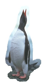
(b) ACDM 1 $\nu_{s}=1.28\cdot 10^{7}$ $\nu_{d}=1.3\cdot 10^{5}$

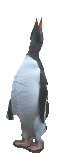
(c) ACDM 20 $\nu_{s}=8.38\cdot 10^{6}$ $\nu_{d}=8.14\cdot 10^{4}$

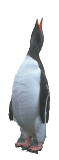
(d) ACDM 100 $\nu_{s}=2.9\cdot 10^{6}$ $\nu_{d}=1.5\cdot 10^{4}$

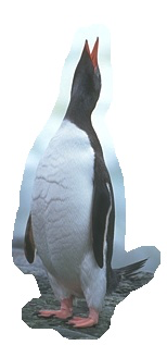
(e) AP 1 $\nu_{s}=9.98\cdot 10^{6}$ $\nu_{d}=1.06\cdot 10^{5}$

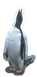
(f) AP 20 $\nu_{s}=8.96\cdot 10^{6}$ $\nu_{d}=1.05\cdot 10^{5}$

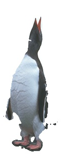
(g) AP 100 $\nu_{s}=7.64\cdot 10^{6}$ $\nu_{d}=8.3\cdot 10^{4}$

Figure 4: Penguin segmentation results for the fastest (ACDM) and slowest (AP) algorithms, after 1, 20, and 100 projections. The $\nu_{s}$ and $\nu_{d}$ values are the smooth and discrete dual gaps.

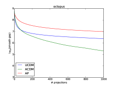
(a) Smooth gaps - Octopus

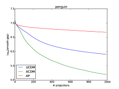
(b) Smooth gaps - Penguin

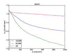
(c) Smooth gaps - Plane

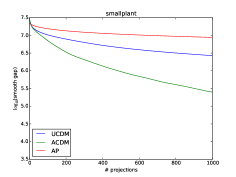
(d) Smooth gaps - Small plant

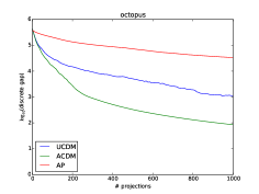
(e) Discrete gaps - Octopus

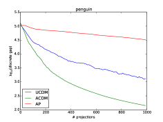
(f) Discrete gaps - Penguin

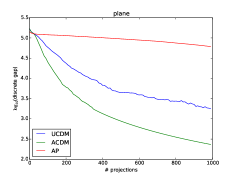
(g) Discrete gaps - Plane

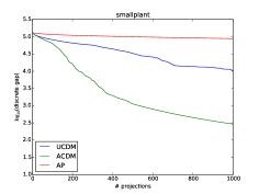
(h) Discrete gaps - Small plant

Figure 5: Comparison of the convergence of the three algorithms (UCDM, ACDM, AP) on four image segmentation instances.

Algorithms. We empirically evaluate and compare the following algorithms: the RCDM described in Section 2, the ACDM described in Section 3, and the alternating projections (AP) algorithm of [12]. The AP algorithm solves the following best approximation problem that is equivalent to (Prox-DSM):

$$\min_{a\in\mathcal{A},y\in\mathcal{Y}}\left\|a-y\right\|^{2}$$ (Best-Approx)

where $\mathcal{A}=\left\{(a^{(1)},a^{(2)},\dots,a^{(r)})\in{\mathbb{R}}^{nr}\colon\sum_{i=1}^{r}a^{(i)}=0\right\}$ and $\mathcal{Y}=\bigotimes_{i=1}^{r}B(F_{i})$.

The AP algorithm starts with a point $a_{0}\in\mathcal{A}$ and it iteratively constructs a sequence $\left\{(a_{k},y_{k})\right\}_{k\geq 0}$ by projecting onto $\mathcal{A}$ and $\mathcal{Y}$: $y_{k}=\Pi_{\mathcal{Y}}(a_{k})$, $a_{k+1}=\Pi_{\mathcal{A}}(y_{k})$.

$\Pi_{K}(\cdotp)$ is the projection operator onto $K$, that is, $\Pi_{K}(x)=\operatornamewithlimits{arg\,min}_{z\in K}\left\|x-z\right\|$. Since $\mathcal{A}$ is a subspace, it is straightforward to project onto $\mathcal{A}$. The projection onto $\mathcal{Y}$ can be implemented using the oracles for the projections $\Pi_{B(F_{i})}$ onto the base polytopes of the functions $F_{i}$.

For all three algorithms, the iteration cost is dominated by the cost of projecting onto the base polytopes $B(F_{i})$. Therefore the total number of such projections is a suitable measure for comparing the algorithms. In each iteration, the RCDM algorithm performs a single projection for a random block $i$ and the ACDM algorithm performs a single projection in expectation. The AP algorithm performs $r$ projections in each iteration, one for each block.

Image Segmentation Experiments. We evaluate the algorithms on graph cut problems that arise in image segmentation or MAP inference tasks in Markov Random Fields. Our experimental setup is similar to that of [6]. We set up the image segmentation problems on a $8$-neighbor grid graph with unary potentials derived from Gaussian Mixture Models of color features [16]. The weight of a graph edge $(i,j)$ between pixels $i$ and $j$ is a function of $\exp(-\left\|v_{i}-v_{j}\right\|^{2})$, where $v_{i}$ is the RGB color vector of pixel $i$. The optimization problem that we solve for each segmentation task is a cut problem on the grid graph.

Function decomposition: We partition the edges of the grid into a small number of matchings and we decompose the function using the cut functions of these matchings. Note that it is straightforward to project onto the base polytopes of such functions using a sequence of projections onto line segments.

Duality gaps: We evaluate the convergence behaviours of the algorithms using the following measures. Let $y$ be a feasible solution to the dual of the proximal problem (Proximal). The solution $x=-\sum_{i=1}^{r}y^{(i)}$ is a feasible solution for the proximal problem. We define the smooth duality gap to be the difference between the objective values of the primal solution $x$ and the dual solution $y$: $\nu_{s}=\left(f(x)+{1\over 2}\left\|x\right\|^{2}\right)-\left(-{r\over 2}\left\|Sy\right\|^{2}\right)$. Additionally, we compute a discrete duality gap for the discrete problem (DSM) and the dual of its Lovász relaxation; the latter is the problem $\max_{z\in B(F)}(z)_{-}(V)$, where $(z)_{-}=\min\left\{z,0\right\}$ applied elementwise [6]. The best level set $S_{x}$ of the proximal solution $x=-\sum_{i=1}^{r}y^{(i)}$ is a solution to the discrete problem (DSM). The solution $z=-x=\sum_{i=1}^{r}y^{(i)}$ is a feasible solution for the dual of the Lovász relaxation. We define the discrete duality gap to be the difference between the objective values of these solutions: $\nu_{d}(x)=F(S_{x})-(-x)_{-}(V)$.

We evaluated the algorithms on four image segmentation instances [7, 16]. Figure 5 shows the smooth and discrete duality gaps on the four instances. Figure 4 shows some segmentation results for one of the instances.

Acknowledgements. We thank Stefanie Jegelka for providing us with some of the data used in our experiments.

Appendix A Proof of Lemma 1

By the definition of the Lovász extension, for each $i\in[r]$, we have

$$f_{i}(x)=\max_{y^{(i)}\in B(F_{i})}\langle y^{(i)},x\rangle.$$

Therefore

$$\min_{x\in{\mathbb{R}}^{n}}\sum_{i=1}^{r}\left(f_{i}(x)+{1\over 2r}\left\|x\right\|^{2}\right)$$

$$=\min_{x\in{\mathbb{R}}^{n}}\sum_{i=1}^{r}\left(\max_{y^{(i)}\in B(F_{i})}\langle y^{(i)},x\rangle+{1\over 2r}\left\|x\right\|^{2}\right)$$

$$=\min_{x\in{\mathbb{R}}^{n}}\max_{y^{(1)}\in B(F_{1}),\dots,y^{(r)}\in B(F_{r})}\sum_{i=1}^{r}\left(\langle y^{(i)},x\rangle+{1\over 2r}\left\|x\right\|^{2}\right)$$

$$=\max_{y^{(1)}\in B(F_{1}),\dots,y^{(r)}\in B(F_{r})}\min_{x\in{\mathbb{R}}^{n}}\sum_{i=1}^{r}\left(\langle y^{(i)},x\rangle+{1\over 2r}\left\|x\right\|^{2}\right)$$

$$=\max_{y^{(1)}\in B(F_{1}),\dots,y^{(r)}\in B(F_{r})}-{1\over 2}\left\|\sum_{i=1}^{r}y^{(i)}\right\|^{2}$$

On the third line, we have used the fact that the function $\langle y,x\rangle+(1/2r)\left\|x\right\|^{2}$ is convex in $x$ and linear in $y$, which allows us to exchange the $\min$ and the $\max$ (see for example Corollary 37.3.2 in Rockafellar [15]). On the fourth line, we have used the fact that the minimum is achieved at $x=-\sum_{i=1}^{r}y^{(i)}$.

Appendix B Proofs omitted from Section 2

If $x\in{\mathbb{R}}^{nr}$ and $\mathcal{X}$ is a subspace of ${\mathbb{R}}^{nr}$, we let $\Pi_{\mathcal{X}}(x)$ denote the projection of $x$ on $\mathcal{X}$, that is, $\Pi_{\mathcal{X}}(x)=\operatornamewithlimits{arg\,min}_{z\in{\mathbb{R}}^{nr}}\left\|x-z\right\|$. We let $\mathcal{X}^{\perp}$ denote the orthogonal complement of the subspace $\mathcal{X}$.

Proposition 9.

For any point $x\in{\mathbb{R}}^{nr}$, $\Pi_{\mathcal{Q}^{\perp}}(x)=S^{T}Sx$ and thus $\Pi_{\mathcal{Q}}(x)=x-S^{T}Sx$.

Proof: Since $\mathcal{Q}$ is the null space of $S$, $\mathcal{Q}^{\perp}$ is the row space of $S$. Since the rows of $S$ are orthonormal, they form a basis for $\mathcal{Q}^{\perp}$. Therefore, if we let $v_{1},\dots,v_{n}$ denote the rows of $S$, we have

$$\Pi_{\mathcal{Q}^{\perp}}(x)=\sum_{i=1}^{n}\langle x,v_{i}\rangle v_{i}=S^{T}Sx.$$

$\Box$

Proposition 10.

The set of all optimal solutions to (Prox-DSM) is equal to $E$.

Proof: We have

$$d(\mathcal{P},\mathcal{Q}) =\min_{y\in\mathcal{P}}\left\|y-\Pi_{\mathcal{Q}}(y)\right\|$$

$$=\min_{y\in\mathcal{P}}\left\|S^{T}Sy\right\|\qquad\textsl{$\langle\!\langle$By Proposition~{}\ref{prop:project-onto-Q}\/$\rangle\!\rangle$}$$

$$=\min_{y\in\mathcal{P}}\left\|Sy\right\|$$

Since (Prox-DSM) is the problem $\min_{y\in\mathcal{P}}r\left\|Sy\right\|^{2}$, $E$ is the set of all optimal solutions to (Prox-DSM). $\Box$

Proposition 11.

Let $y\in{\mathbb{R}}^{nr}$ and let $p\in E$. We have $d(y,\mathcal{Q}^{\prime})=\left\|S(y-p)\right\|$.

Proof: Since $\mathcal{Q}^{\prime}=\mathcal{Q}-v$, we have

$$d(y,\mathcal{Q}^{\prime}) =d(y+v,\mathcal{Q})$$

$$=\left\|\Pi_{\mathcal{Q}^{\perp}}(y+v)\right\|$$

$$=\left\|S^{T}S(y+v)\right\|\qquad\textsl{$\langle\!\langle$By Proposition~{}{\ref{prop:project-onto-Q}}\/$\rangle\!\rangle$}$$

$$=\left\|S^{T}S(y-S^{T}Sp)\right\|\qquad\textsl{$\langle\!\langle$Since $v=-S^{T}Sp$\/$\rangle\!\rangle$}$$

$$=\left\|S^{T}S(y-p)\right\|\qquad\textsl{$\langle\!\langle$Since $SS^{T}=I_{n}$\/$\rangle\!\rangle$}$$

$$=\left\|S(y-p)\right\|$$

$\Box$

References

[1]
Francis Bach.
Learning with submodular functions: A convex optimization
perspective.
ArXiv preprint arXiv:1111.6453, 2011.
[2]
Olivier Fercoq and Peter Richtárik.
Accelerated, parallel and proximal coordinate descent.
ArXiv preprint arXiv:1312.5799, 2013.
[3]
Lisa Fleischer and Satoru Iwata.
A push-relabel framework for submodular function minimization and
applications to parametric optimization.
Discrete Applied Mathematics, 131(2):311–322, 2003.
[4]
Martin Grötschel, László Lovász, and Alexander Schrijver.
The ellipsoid method and its consequences in combinatorial
optimization.
Combinatorica, 1(2):169–197, 1981.
[5]
Satoru Iwata.
A faster scaling algorithm for minimizing submodular functions.
SIAM Journal on Computing, 32(4):833–840, 2003.
[6]
Stefanie Jegelka, Francis Bach, and Suvrit Sra.
Reflection methods for user-friendly submodular optimization.
In Advances in Neural Information Processing Systems (NIPS),
pages 1313–1321, 2013.
[7]
Stefanie Jegelka and Jeff Bilmes.
Submodularity beyond submodular energies: coupling edges in graph
cuts.
In Computer Vision and Pattern Recognition (CVPR), 2011 IEEE
Conference on, pages 1897–1904. IEEE, 2011.
[8]
Vladimir Kolmogorov.
Minimizing a sum of submodular functions.
Discrete Applied Mathematics, 160(15):2246–2258, 2012.
[9]
László Lovász.
Submodular functions and convexity.
In Mathematical Programming The State of the Art, pages
235–257. Springer, 1983.
[10]
Yu. Nesterov.
Efficiency of coordinate descent methods on huge-scale optimization
problems.
SIAM Journal on Optimization, 22(2):341–362, 2012.
[11]
Yurii Nesterov.
Introductory lectures on convex optimization: A basic course,
volume 87.
Springer, 2004.
[12]
Robert Nishihara, Stefanie Jegelka, and Michael I Jordan.
On the convergence rate of decomposable submodular function
minimization.
In Advances in Neural Information Processing Systems (NIPS),
pages 640–648, 2014.
[13]
Robert Nishihara, Stefanie Jegelka, and Michael I Jordan.
On the convergence rate of decomposable submodular function
minimization.
ArXiv preprint arXiv:1406.6474, 2014.
[14]
James B Orlin.
A faster strongly polynomial time algorithm for submodular function
minimization.
Mathematical Programming, 118(2):237–251, 2009.
[15]
R Tyrrell Rockafellar.
Convex analysis.
Number 28 in Princeton Mathematical Series. Princeton university
press, 1970.
[16]
Carsten Rother, Vladimir Kolmogorov, and Andrew Blake.
Grabcut: Interactive foreground extraction using iterated graph cuts.
ACM Transactions on Graphics (TOG), 23(3):309–314, 2004.
[17]
Alexander Schrijver.
A combinatorial algorithm minimizing submodular functions in strongly
polynomial time.
Journal of Combinatorial Theory, Series B, 80(2):346–355,
2000.
[18]
Alexander Schrijver.
Combinatorial optimization: polyhedra and efficiency,
volume 24.
Springer Science & Business Media, 2003.
[19]
Peter Stobbe and Andreas Krause.
Efficient minimization of decomposable submodular functions.
In Advances in Neural Information Processing Systems (NIPS),
pages 2208–2216, 2010.