One-armed spirals in locally isothermal, radially structured self-gravitating discs

Abstract

We describe a new mechanism that leads to the destabilisation of non-axisymmetric waves in astrophysical discs with an imposed radial temperature gradient. This might apply, for example, to the outer parts of protoplanetary discs. We use linear density wave theory to show that non-axisymmetric perturbations generally do not conserve their angular momentum in the presence of a forced temperature gradient. This implies an exchange of angular momentum between linear perturbations and the background disc. In particular, when the disturbance is a low-frequency trailing wave and the disc temperature decreases outwards, this interaction is unstable and leads to the growth of the wave. We demonstrate this phenomenon through numerical hydrodynamic simulations of locally isothermal discs in 2D using the FARGO code and in 3D with the ZEUS-MP and PLUTO codes. We consider radially structured discs with a self-gravitating region which remains stable in the absence of a temperature gradient. However, when a temperature gradient is imposed we observe exponential growth of a one-armed spiral mode (azimuthal wavenumber $m=1$) with co-rotation radius outside the bulk of the spiral arm, resulting in a nearly-stationary one-armed spiral pattern. The development of this one-armed spiral does not require the movement of the central star, as found in previous studies. Because destabilisation by a forced temperature gradient does not explicitly require disc self-gravity, we suggest this mechanism may also affect low-frequency one-armed oscillations in non-self-gravitating discs.

1 Introduction

An exciting development in the study of circumstellar discs is the direct observation of large-scale, non-axisymmetric structures within them. These include lopsided dust distributions (van der Marel et al., 2013; Fukagawa et al., 2013; Casassus et al., 2013; Isella et al., 2013; Pérez et al., 2014; Follette et al., 2014; van der Plas et al., 2014) and spiral arms (Hashimoto et al., 2011; Muto et al., 2012; Boccaletti et al., 2013; Grady et al., 2013; Christiaens et al., 2014; Avenhaus et al., 2014).

The attractive explanation for asymmetries in circumstellar discs is disc-planet interaction. In particular, spiral structures naturally arise from the gravitational interaction between a planet and the gaseous protoplanetary disc it is embedded in (see, e.g. Baruteau et al., 2013, for a recent review). Thus, the presence of spiral arms in circumstellar discs could be signposts of planet formation (but see Juhasz et al., 2014).

Spiral arms are also characteristic of global gravitational instability (GI) in differentially rotating discs (Goldreich & Lynden-Bell, 1965; Laughlin & Rozyczka, 1996; Laughlin, Korchagin & Adams, 1998; Nelson et al., 1998; Lodato & Rice, 2005; Forgan et al., 2011). Large-scale spiral arms can provide significant angular momentum transport necessary for mass accretion (Lynden-Bell & Kalnajs, 1972; Papaloizou & Savonije, 1991; Balbus & Papaloizou, 1999; Lodato & Rice, 2004), and spiral structures due to GI are potentially observable with the Atacama Large Millimeter/sub-millimeter Array (Cossins, Lodato & Testi, 2010; Dipierro et al., 2014). GI can be expected in the earliest stages of circumstellar disc formation (Kratter et al., 2010; Inutsuka, Machida & Matsumoto, 2010; Tsukamoto, Machida & Inutsuka, 2013), and may be possible in the outer parts of the disc (Rafikov, 2005; Matzner & Levin, 2005; Kimura & Tsuribe, 2012).

Single-arm spirals, or eccentric modes, corresponding to perturbations with azimuthal wavenumber $m=1$, have received interest in the context of protoplanetary discs because of their global nature (Adams, Ruden & Shu, 1989; Heemskerk, Papaloizou & Savonije, 1992; Laughlin & Korchagin, 1996; Tremaine, 2001; Papaloizou, 2002; Hopkins, 2010). In the ‘SLING’ mechanism proposed by Shu et al. (1990), an $m=1$ gravitational instability arises from the motion of the central star induced by the one-armed perturbation, and requires a massive disc (the former may have observable consequences, Michael & Durisen, 2010).

In this work we identify a new mechanism that leads to the growth of one-armed spirals in astrophysical discs. We show that when the disc temperature is prescribed (called locally isothermal discs), the usual statement of the conservation of angular momentum for linear perturbations acquires a source term proportional to the temperature gradient. This permits angular momentum exchange between linear perturbations and the background disc. This ‘background torque’ can destabilise low-frequency non-axisymmetric trailing waves when the disc temperature decreases outwards.

We employ direct hydrodynamic simulations using three different grid-based codes to demonstrate how this ‘background torque’ can lead to the growth of one-armed spirals in radially structured, self-gravitating discs. This is despite the fact that our disc models do not meet the requirements for the ‘SLING’ mechanism. Although our numerical simulations consider self-gravitating discs, this ‘background torque’ is generic for locally isothermal discs and its existence does not require disc self-gravity. Thus, the destabilisation effect we describe should also be applicable to non-self-gravitating discs.

This paper is organised as follows. In §2 we describe the system of interest and list the governing equations. In §3 we use linear theory to show how a fixed temperature profile can destabilise non-axisymmetric waves in discs. §4 describes the numerical setup and hydrodynamic codes we use to demonstrate the growth of one-armed spirals due to an imposed temperature gradient. Our simulation results are presented in §5 for two-dimensional (2D) discs and in §6 for three-dimensional (3D) discs, and we further discuss them in §7. We summarise in §8 with some speculations for future work.

2 Governing equations

We consider an inviscid fluid disc of mass $M_{d}$ orbiting a central star of mass $M_{*}$. We will mainly examine 2D (or razor-thin) discs in favour of numerical resolution, but have also carried out some 3D disc simulations. Hence, for generality we describe the system in 3D, using both cylindrical $(R,\phi,z)$ and spherical polar coordinates $(r,\theta,\phi)$ centred on the star. The governing fluid equations in 3D are

$$\frac{\partial\rho}{\partial t}+\nabla\cdot\left(\rho\bm{v}\right)=0,$$ (1)

$$\frac{\partial\bm{v}}{\partial t}+\bm{v}\cdot\nabla\bm{v}=-\frac{1}{\rho}\nabla p-\nabla\Phi_{\mathrm{tot}},$$ (2)

$$\nabla^{2}\Phi_{d}=4\pi G\rho,$$ (3)

where $\rho$ is the mass density, $\bm{v}$ is the fluid velocity (the angular velocity being $\Omega\equiv v_{\phi}/R$), $p$ is the pressure and the total potential $\Phi_{\mathrm{tot}}=\Phi_{*}+\Phi_{d}$ consists of that from the central star,

$$\Phi_{*}(r)=-\frac{GM_{*}}{r},$$ (4)

where $G$ is the gravitational constant, and the disc potential $\Phi_{d}$. We impose a locally isothermal equation of state

$$p=c_{s}^{2}(R)\rho,$$ (5)

where the sound-speed $c_{s}$ is given by

$$c_{s}(R)=c_{s0}\left(\frac{R}{R_{0}}\right)^{-q/2}$$ (6)

where $c_{s0}=hR_{0}\Omega_{k}(R_{0})$ and $h$ is the disc aspect-ratio at the reference radius $R=R_{0}$, $\Omega_{k}=\sqrt{GM_{*}/R^{3}}$ is the midplane Keplerian frequency, and $-q$ is the imposed temperature gradient since, for an ideal gas the temperature is proportional to $c_{s}^{2}$. For convenience we will refer to $c_{s}^{2}$ as the disc temperature. The vertical disc scale-height is defined by $H=c_{s}/\Omega_{k}$. Thus, a strictly isothermal disc with $q=0$ has $H\propto R^{3/2}$, and $q=1$ corresponds to a disc with constant $H/R$.

The 2D disc equations are obtained by replacing $\rho$ with the surface mass density $\Sigma$, $p$ becomes the vertically-integrated pressure, and the 2D fluid velocity $\bm{v}$ is evaluated at the midplane, as are the forces in the momentum equations. In the Poisson equation, $\rho$ is replaced by $\Sigma\delta(z)$, where $\delta(z)$ is the delta function.

3 Linear density waves

We describe a key feature of locally isothermal discs that enables angular momentum exchange between small disturbances and the background disc through an imposed radial temperature gradient. This conclusion results from the consideration of angular momentum conservation within the framework of linear perturbation theory. For simplicity, in this section we consider 2D discs.

In a linear analysis, one assumes a steady axisymmetric background state, which is then perturbed such that

$$\Sigma\to\Sigma(R)+\delta\Sigma_{m}(R)\exp{\left[\mathrm{i}\left(-\sigma t+m\phi\right)\right]},$$ (7)

and similarly for other variables, where $\sigma=\omega+\mathrm{i}\gamma$ is a complex frequency with $\omega$ being the real frequency, $\gamma$ the growth rate, and $m$ is an integer. We take $m>0$ without loss of generality.

The linearised mass and momentum equations are

$$-\mathrm{i}\bar{\sigma}\delta\Sigma_{m}=-\frac{1}{R}\frac{d}{dR}\left(R\Sigma\delta v_{Rm}\right)-\frac{\mathrm{i}m\Sigma}{R}\delta v_{\phi m},$$ (8)

$$-\mathrm{i}\bar{\sigma}\delta v_{Rm}-2\Omega\delta v_{\phi m}=-c_{s}^{2}(R)\frac{d}{dR}\left(\frac{\delta\Sigma_{m}}{\Sigma}\right)-\frac{d}{dR}\delta\Phi_{m},$$ (9)

$$-\mathrm{i}\bar{\sigma}\delta v_{\phi m}+\frac{\kappa^{2}}{2\Omega}\delta v_{Rm}=-\frac{\mathrm{i}m}{R}\left(c_{s}^{2}\frac{\delta\Sigma_{m}}{\Sigma}+\delta\Phi_{m}\right),$$ (10)

where $\bar{\sigma}=\sigma-m\Omega$ and $\kappa^{2}=R^{-3}\partial_{R}(R^{4}\Omega^{2})$ is the square of the epicyclic frequency. A locally isothermal equation of state has been assumed in Eq. 9. The linearised Poisson equation is

$$\nabla^{2}\delta\Phi_{m}=4\pi G\delta\Sigma_{m}\delta(z).$$ (11)

These linearised equations can be combined into a single integro-differential equation eigenvalue problem. We defer a full numerical exploration of the linear problem to a future study. Here, we discuss some general properties of the linear perturbations.

3.1 Global angular momentum conservation for linear perturbations

It can be shown that linear perturbations with $\phi$-dependence in the form $\exp{(\mathrm{i}m\phi)}$ satisfies angular momentum conservation in the form

$$\frac{\partial j_{\mathrm{lin}}}{\partial t}+\nabla\cdot\bm{F}=T_{\mathrm{BG}},$$ (12)

(e.g. Narayan, Goldreich & Goodman, 1987; Ryu & Goodman, 1992; Lin, Papaloizou & Kley, 1993) where

$$j_{\mathrm{lin}}\equiv-\frac{m\Sigma}{2}\operatorname{Im}\left(\bm{\xi}^{*}\cdot\frac{\partial\bm{\xi}}{\partial t}+\Omega\hat{\bm{k}}\cdot\bm{\xi}\times\bm{\xi}^{*}+\mathrm{i}m\Omega|\bm{\xi}|^{2}\right)$$ (13)

is the angular momentum density of the linear disturbance (which may be positive or negative), $\bm{\xi}$ is the Lagrangian displacement and ^∗ denotes complex conjugation, and $\bm{F}$ is the vertically-integrated angular momentum flux consisting of a Reynolds stress and a gravitational stress (Lin & Papaloizou, 2011). Explicit expressions for $\bm{\xi}$ can be found in, e.g. Papaloizou & Pringle (1985).

In Eq. 12, the background torque density $T_{\mathrm{BG}}$ is

$$T_{\mathrm{BG}}\equiv-\frac{m}{2}\operatorname{Im}\left(\delta\Sigma_{m}\xi_{R}^{*}\frac{dc_{s}^{2}}{dR}\right),$$ (14)

and arises because we have adopted a locally isothermal equation of state in the perturbed disc. We outline the derivation of $T_{\mathrm{BG}}$ in Appendix A.

In a barotropic fluid, such as a strictly isothermal disc, $T_{\mathrm{BG}}$ vanishes and the total angular momentum associated with the perturbation is conserved, provided that there is no net angular momentum flux. However, as noted in Lin & Papaloizou (2011), if there is an imposed temperature gradient, as in the disc models we consider, then $T_{\mathrm{BG}}\neq 0$ in general, which corresponds to a local torque exerted by the background disc on the perturbation.

The important consequence of the background torque is the possibility of instability if $T_{\mathrm{BG}}j_{\mathrm{lin}}>0$. That is, if $j_{\mathrm{lin}}$ is positive (negative) and $T_{\mathrm{BG}}$ is also positive (negative), then the local angular momentum density of the linear disturbance will further increase (decrease) with time. This implies the amplitude of the disturbance may grow by exchanging angular momentum with the background disc.

We demonstrate instability for low-frequency modes ($|\omega|\ll m\Omega$) by explicitly showing its angular momentum density $j_{\mathrm{lin}}<0$, and the background torque $T_{\mathrm{BG}}<0$ for appropriate perturbations and radial temperature gradients.

3.2 Angular momentum density of non-axisymmetric low-frequency modes

From Eq. 13 and assuming a time-dependence of the form $\exp{(-\mathrm{i}\sigma t)}$ with $\operatorname{Re}{\sigma}=\omega$, the angular momentum density associated with linear waves is

$$j_{\mathrm{lin}}=\frac{m\Sigma}{2}\left[\left(\omega-m\Omega\right)|\bm{\xi}|^{2}+\mathrm{i}\Omega\left(\xi_{R}\xi_{\phi}^{*}-\xi_{R}^{*}\xi_{\phi}\right)\right].$$ (15)

For a low-frequency mode, $|\omega|\ll m\Omega$. Then neglecting the term $\omega|\bm{\xi}|^{2}$, we find

$$j_{\mathrm{lin}} \simeq\frac{m\Sigma\Omega}{2}\left[-m|\bm{\xi}|^{2}+\mathrm{i}\left(\xi_{R}\xi_{\phi}^{*}-\xi_{R}^{*}\xi_{\phi}\right)\right]$$

$$=-\frac{m\Sigma\Omega}{2}\left[(m-1)|\bm{\xi}|^{2}+|\xi_{R}+\mathrm{i}\xi_{\phi}|^{2}\right].$$ (16)

Thus, non-axisymmetric ($m\geq 1$) low-frequency modes generally have negative angular momentum. If the mode loses (positive) angular momentum to the background, then we can expect instability. We show below how this is possible through a forced temperature gradient via the background torque. It is simplest to calculate $T_{\mathrm{BG}}$ in the local approximation, which we review first.

3.3 Local results

In the local approximation, perturbations are assumed to vary rapidly relative to any background gradients. The dispersion relation for tightly-wound density waves of the form $\exp{[\mathrm{i}(-\sigma t+m\phi+kR)]}$ in a razor-thin disc is

$$(\sigma-m\Omega)^{2}=\kappa^{2}+k^{2}c_{s}^{2}-2\pi G\Sigma|k|,$$ (17)

where $k$ is a real wavenumber such that $|kR|\gg 1$ (Shu, 1991). Note that in the strictly local approximation, where all global effects are neglected, only axisymmetric perturbations ($m=0$) can be unstable.

Given the real frequency $\omega$ or pattern speed $\Omega_{p}\equiv\omega/m$ of a non-axisymmetric neutral mode , Eq. 17 can be solved for $|k|$,

$$|k|=k_{c}\left[1\pm\sqrt{1-Q^{2}(1-\nu^{2})}\right],$$ (18)

where

$$k_{c}\equiv\frac{\pi G\Sigma}{c_{s}^{2}}$$ (19)

is a characteristic wavenumber,

$$Q\equiv\frac{c_{s}\kappa}{\pi G\Sigma}$$ (20)

is the usual Toomre parameter, and

$$\nu\equiv\frac{(\omega-m\Omega)}{\kappa}$$ (21)

is a dimensionless frequency. In Eq. 18, the upper (lower) sign correspond to short (long) waves, and $k>0$ ($k<0$) correspond to trailing (leading) waves.

At the co-rotation radius $R_{c}$ the pattern speed matches the fluid rotation,

$$\Omega(R_{c})=\Omega_{p}.$$ (22)

Lindblad resonances $R_{L}$ occurs where

$$\nu^{2}(R_{L})=1.$$ (23)

Finally, Q-barriers occur at radii $R_{Qb}$ where

$$Q^{2}(R_{Qb})\left[1-\nu^{2}(R_{Qb})\right]=1.$$ (24)

According to Eq. 18, purely wave-like solutions with real $k$ are only possible where $Q^{2}(1-\nu^{2})\leq 1$.

A detailed discussion of the properties of local density waves is given in Shu (1991). An important result, which holds for waves of all frequencies, is that waves interior to co-rotation ($R<R_{c}$) have negative angular momentum, while waves outside co-rotation ($R>R_{c}$) have positive angular momentum.

3.4 Unstable interaction between low-frequency modes and the background disc due to an imposed temperature gradient

Here we show that the torque density acting on a local mode due to the background temperature gradient can be negative, which would enforce low-frequency modes, because they have negative angular momentum.

The Eulerian surface density perturbation is given by

$$\delta\Sigma_{m}=-\nabla\cdot\left(\Sigma\bm{\xi}\right)=-\frac{1}{R}\frac{d}{dR}\left(R\Sigma\xi_{R}\right)-\frac{\mathrm{i}m}{R}\Sigma\xi_{\phi}.$$ (25)

We invoke local theory by setting $d/dR\to\mathrm{i}k$ where $k$ is real, and assume $|kR|\gg m$ so that the second term on the right hand side of Eq. 25 can be neglected. Then

$$\delta\Sigma_{m}\simeq-\mathrm{i}k\Sigma\xi_{R}.$$ (26)

Inserting this into the expression for the background torque, Eq. 14, we find

$$T_{\mathrm{BG}}=\frac{m}{2}\frac{dc_{s}^{2}}{dR}k\Sigma|\xi_{R}|^{2}.$$ (27)

This torque density is negative for trailing waves ($k>0$) in discs with a fixed temperature profile decreasing outwards ($dc_{s}^{2}/dR<0$). Note that this conclusion does not rely on the low-frequency approximation.

However, if the linear disturbance under consideration is a low-frequency mode, then it has negative angular momentum. If it is trailing and $dc_{s}^{2}/dR<0$, as is typical in astrophysical discs, then $T_{\mathrm{BG}}<0$ and the background disc applies a negative torque on the disturbance, which further decreases its angular momentum. This suggests the mode amplitude will grow.

Using $j_{\mathrm{lin}}$ and $T_{\mathrm{BG}}$, we can estimate the growth rate $\gamma$ of linear perturbations due to the background torque as

$$2\gamma\sim\frac{T_{\mathrm{BG}}}{j_{\mathrm{lin}}},$$ (28)

where the factor of two accounts for the fact that the angular momentum density is quadratic in the linear perturbations. Inserting the above expressions for $j_{\mathrm{lin}}$ and $T_{\mathrm{BG}}$ for gives

$$2\gamma\sim-\frac{dc_{s}^{2}}{dR}\frac{k}{\Omega}\frac{|\xi_{R}|^{2}}{\left[(m-1)|\bm{\xi}|^{2}+|\xi_{R}+\mathrm{i}\xi_{\phi}|^{2}\right]}=-\frac{dc_{s}^{2}}{dR}\frac{k}{m\Omega},$$ (29)

where the second equality uses $\xi_{\phi}\simeq 2\mathrm{i}\xi_{R}/m$ for low-frequency modes in the local approximation, as shown in Appendix B. Then for the temperature profiles $c_{s}^{2}=c_{s0}^{2}(R/R_{0})^{-q}$ as adopted in our disc models,

$$2\gamma\sim q\frac{c_{s}^{2}}{R}\frac{k}{m\Omega}\sim qh\left(\frac{kH}{m}\right)\Omega,$$ (30)

where we used $c_{s}\sim H\Omega\sim hR\Omega$. Eq. 30 suggests that perturbations with small radial length-scales ($kH\;\raisebox{-3.44444pt}{$\buildrel\textstyle>\over{\sim}$}\;m$) are most favourable for destabilisation. Taking the local approximation is then appropriate.

Note that the derivation of Eq. 27 and Eq. 30 do not require the disc to be self-gravitating. Thus, destabilisation by the background torque is not directly associated with disc self-gravity. However, in order to evaluate Eq. 27 or Eq. 30 in terms of disc parameters (as done in §5.3), we need to insert a value of $k$, which may depend on disc self-gravity (e.g. from Eq. 18).

4 Numerical simulations

We demonstrate the destabilising effect of a fixed temperature gradient using numerical simulations. The above discussion is generic for low-frequency non-axisymmetric modes, but for simulations we will consider specific examples.

There are two parts to the destabilising mechanism: the disc should support low-frequency modes, which is then destabilised by an imposed temperature gradient. The latter is straight forward to implement by adopting a locally isothermal equation of state as described in §2. For the former, we consider discs with a radially-structured Toomre $Q$ profile. We use local theory to show that such discs can trap low-frequency one-armed ($m=1$) modes. This is convenient because Eq. 30 indicates that modes with small $m$ are more favourable for destabilisation.

4.1 Disc model and initial conditions

For the initial disc profile we adopt a modified power-law disc with surface density given by

$$\Sigma(R)=\Sigma_{\mathrm{ref}}\left(\frac{R}{R_{0}}\right)^{-s}\times B(R;R_{1},R_{2},\epsilon,\delta R),$$ (31)

where $s$ is the power-law index describing the smooth disc and $\Sigma_{\mathrm{ref}}$ is a surface density scale chosen by specifying $Q_{\mathrm{out}}$, the Keplerian Toomre parameter at $R=R_{2}$,

$$Q_{\mathrm{out}}=\left.\frac{c_{s}\Omega_{k}}{\pi G\Sigma}\right|_{R=R_{2}}.$$ (32)

The bump function $B(R)$ represents a surface density boost between $R\in[R_{1},R_{2}]$ by a factor $\epsilon^{-1}>1$, and $\delta R$ is the transition width between the bump and the smooth disc. We choose

$$B(R)=f_{1}(R)\times f_{2}(R),$$ (33)

$$f_{1}(R)=\frac{1}{2}\left(1-\epsilon\right)\left[1+\tanh\left(\frac{R-R_{1}}{\Delta_{1}}\right)\right]+\epsilon,$$ (34)

$$f_{2}(R)=\frac{1}{2}\left(1-\epsilon\right)\left[1-\tanh\left(\frac{R-R_{2}}{\Delta_{2}}\right)\right]+\epsilon,$$ (35)

where $\Delta_{1,2}=\delta R\times H(R_{1,2})$.

The 3D disc structure is obtained by assuming vertical hydrostatic balance

$$0=\frac{1}{\rho}\frac{\partial p}{\partial z}+\frac{\partial\Phi_{*}}{\partial z}+\frac{\partial\Phi_{d}}{\partial z},$$ (36)

which gives the mass density as

$$\rho=\frac{\Sigma}{\sqrt{2\pi}H}Z(R,z),$$ (37)

where $Z(R,z)$ describes vertical stratification. In practice, we numerically solve for $Z(R,z)$ by neglecting the radial self-gravity force compared to vertical self-gravity, which reduces the equations for vertical hydrostatic equilibrium to ordinary differential equations. This procedure is described in Lin (2012).

Our fiducial parameter values are: $s=2$, $R_{1}=R_{0}$, $R_{2}=2R_{0}$, $\epsilon=0.1$, $\delta R=5$, $h=0.05$ and $Q_{\mathrm{out}}=2$. An example of the initial surface density and the Toomre $Q$ parameter is shown in Fig. 1. Since $Q>1$, the disc is stable to local axisymmetric perturbations (Toomre, 1964). The transition between self-gravitating and non-self-gravitating portions of the disc occur smoothly across $\sim 10H$. Initially there is no vertical or radial velocity ($v_{R}=v_{r}=v_{\theta}=0$). The azimuthal velocity is initialized to satisfy centrifugal balance with pressure and gravity,

$$\frac{v_{\phi}^{2}}{r}=\frac{1}{\rho}\frac{\partial p}{\partial r}+\frac{\partial\Phi_{\mathrm{tot}}}{\partial r}$$ (38)

and similarly in 2D.

Figure 1: Fiducial profiles of the surface density (top) and Toomre parameter (bottom) used in this work.

4.2 Codes

We use three independent grid-based codes to simulate the above system. We adopt computational units such that $G=M_{*}=R_{0}=1$. Time is measured in the Keplerian orbital period at the reference radius, $P_{0}\equiv 2\pi/\Omega_{k}(R_{0})$.

4.2.1 FARGO

Our primary code is FARGO with self-gravity (Baruteau & Masset, 2008). This is a popular, simple finite-difference code for 2D discs. ‘FARGO’ refers to its azimuthal transport algorithm, which removes the mean azimuthal velocity of the disc, thereby permit larger time-steps than that would otherwise be allowed by the usual Courant condition based on the full azimuthal velocity (Masset, 2000a, b).

The 2D disc occupies $R\in[R_{\mathrm{min}},R_{\mathrm{max}}],\,\phi\in[0,2\pi]$ and is divided into $(N_{R},N_{\phi})$ grids, logarithmically spaced in radius and uniformly spaced in azimuth. At radial boundaries we set the hydrodynamic variables to their initial values.

The 2D Poisson equation is solved in integral form,

$$\Phi_{d,z=0}(R,\phi)$$

$$=-\int_{R_{\mathrm{min}}}^{R_{\mathrm{max}}}\int_{0}^{2\pi}\frac{G\Sigma(R^{\prime},\phi^{\prime})R^{\prime}dR^{\prime}d\phi^{\prime}}{\sqrt{R^{2}+R^{\prime 2}-2RR^{\prime}\cos{(\phi-\phi^{\prime})}+\epsilon_{g}^{2}}},$$ (39)

using Fast Fourier Transform (FFT), where $\epsilon_{g}$ is a softening length to prevent a numerical singularity. The FFT approach requires $\epsilon_{g}\propto R$ (Baruteau & Masset, 2008). In FARGO, $\epsilon_{g}$ is set to a fraction of $hR$.

4.2.2 ZEUS-MP

ZEUS-MP is a general-purpose finite difference code (Hayes et al., 2006). We use the code in 3D spherical geometry, covering $r\in[r_{\mathrm{min}},r_{\mathrm{max}}]$, $\theta\in[\theta_{\mathrm{min}},\pi/2]$, $\phi\in[0,2\pi]$. The vertical domain is chosen to cover $n_{H}$ scale-heights at $R=R_{0}$, i.e. $\tan{(\pi/2-\theta_{\mathrm{min}})}/h=n_{H}$. The grid is logarithmically spaced in radius and uniformly spaced in the angular coordinates. We assume symmetry across the midplane, and apply reflective boundary conditions at radial boundaries and the upper disc boundary.

ZEUS-MP solves the 3D Poisson equation using a conjugate gradient method. To supply boundary conditions to the linear solver, we expand the boundary potential in spherical harmonics $Y_{lm}$ as described in Boss (1980). The expansion is truncated at $(l,m)=(l_{\mathrm{max}},m_{\mathrm{max}})$. This code was used in Lin (2012) for self-gravitating disc-planet simulations.

4.2.3 PLUTO

PLUTO is a general-purpose Godunov code (Mignone et al., 2007). The grid setup is the same as that adopted in ZEUS-MP above. We configure the code similarly to that used in Lin (2014): piece-wise linear reconstruction, a Roe solver and second order Runge-Kutta time integration. We also enable the FARGO algorithm for azimuthal transport.

We solve the 3D Poisson equation throughout the domain using spherical harmonic expansion (Boss, 1980), as used for the boundary potential in ZEUS-MP. This version of PLUTO was used in Lin & Cloutier (2014) for self-gravitating disc-planet simulations, producing similar results to that of ZEUS-MP and FARGO.

4.3 Diagnostics

4.3.1 Evolution of non-axisymmetric modes

The disc evolution is quantified using mode amplitudes and angular momenta as follows. We list the 2D definitions with obvious 3D generalisations. A hydrodynamic variable $f$ (e.g. $\Sigma$) is written as

$$f(R,\phi,t) =\sum_{m=-\infty}^{\infty}f_{m}(R,t)\exp{\mathrm{i}m\phi}$$

$$=f_{0}+2\operatorname{Re}\left[\sum_{m=1}^{\infty}f_{m}\exp{(\mathrm{i}m\phi)}\right],$$ (40)

where the $f_{m}$ may be obtained from Fourier transform in $\phi$.

The normalised surface density with azimuthal wavenumber $m$ is

$$\Delta\Sigma_{m}=\frac{2}{\Sigma_{00}}\operatorname{Re}\left[\Sigma_{m}\exp{(\mathrm{i}m\phi)}\right]$$ (41)

where $\Sigma_{00}=\Sigma_{0}(t=0)$. The time evolution of the $m^{\mathrm{th}}$ mode can be characterized by assuming $\Sigma_{m}\propto\exp{(-\mathrm{i}\sigma t)}$ as in linear theory. The total non-axisymmetric surface density is

$$\Delta\Sigma=\frac{\Sigma-\Sigma_{0}}{\Sigma_{0}}.$$ (42)

4.3.2 Angular momentum decomposition

The total disc angular momentum is

$$J =\int_{R_{\mathrm{min}}}^{R_{\mathrm{max}}}\int_{0}^{2\pi}\Sigma Rv_{\phi}RdRd\phi$$

$$=2\pi\int_{R_{\mathrm{min}}}^{R_{\mathrm{max}}}R\Sigma_{0}v_{\phi 0}RdR$$

$$\phantom{=}+\sum_{m=1}^{\infty}2\pi\int_{R_{\mathrm{min}}}^{R_{\mathrm{max}}}2R\operatorname{Re}\left[\Sigma_{m}v_{\phi m}^{*}\right]RdR=\sum_{m=0}^{\infty}J_{m}.$$ (43)

We will refer to $J_{m}$ as the $m^{\mathrm{th}}$ component of the total angular momentum, and use it to monitor numerical angular momentum conservation in the simulations. It is important to distinguish this empirical definition from the angular momentum of linear perturbations given in §3, which is defined through a conservation law.

4.3.3 Three-dimensionality

In 3D simulations we measure the importance of vertical motion with $\Theta$, where

$$\Theta^{2}\equiv\frac{\langle v_{z}^{2}\rangle}{\langle v_{R}^{2}\rangle+\langle v_{\phi}^{2}\rangle},$$ (44)

and $\langle\cdot\rangle$ denotes the density-weighted average, e.g.,

$$\langle v_{z}^{2}\rangle\equiv\frac{\int_{R_{1}}^{R_{2}}\int_{\theta_{\mathrm{min}}}^{\pi/2}\int_{0}^{2\pi}\rho v_{z}^{2}dV}{\int_{R_{1}}^{R_{2}}\int_{\theta_{\mathrm{min}}}^{\pi/2}\int_{0}^{2\pi}\rho dV},$$ (45)

and similarly for the horizontal velocities. Thus $\Theta$ is the ratio of the average kinetic energy associated with vertical motion to that in horizontal motion. The radial range of integration is taken over $r\in[R_{1},R_{2}]$ since this is where we find the perturbations to be confined.

5 Results

We first present results from FARGO simulations. The 2D disc spans $[R_{\mathrm{min}},R_{\mathrm{max}}]=[0.4,10]R_{0}$. This gives a total disc mass $M_{d}=0.086M_{*}$. The mass within $R\in[R_{\mathrm{min}},R_{1}]$ is $0.017M_{*}$, that within $R\in[R_{1},R_{2}]$ is $0.049M_{*}$, and that within $R\in[R_{2},R_{\mathrm{max}}]$ is $0.021M_{*}$. We use a resolution of $N_{R}\times N_{\phi}=1024\times 2048$, or about $16$ grids per $H$, and adopt $\epsilon_{g}=10^{-4}hR$ for the self-gravity softening length.

In these simulations the disc is subject to initial perturbations in cylindrical radial velocity,

$$v_{R}\to v_{R}+c_{s}\frac{\delta}{M}\exp{\left[-\frac{1}{2}\left(\frac{R-\overline{R}}{\Delta R}\right)^{2}\right]}\sum_{m=1}^{M}\cos{m\phi},$$ (46)

where the amplitude $\delta\in[-10^{-3},10^{-3}]$ is set randomly but independent of $\phi$, $\overline{R}=(R_{1}+R_{2})/2$ and $\Delta R=(R_{2}-R_{1})/2$.

5.1 Reference run

To obtain a picture of the overall disc evolution, we describe a fiducial run initialised with $M=10$ in Eq. 46. Fig. 2 plots evolution of the maximum non-axisymmetric surface density amplitudes in $R\in[R_{1},R_{2}]$ for $m\in[1,10]$. Snapshots from the simulation are shown in Fig. 3. At early times $t\;\raisebox{-3.44444pt}{$\buildrel\textstyle<\over{\sim}$}\;100P_{0}$ the disc is dominated by low-amplitude high-$m$ perturbations. The $m\geq 4$ modes growth initially and saturate (or decays) after $t=40P_{0}$. Notice the low $m\leq 2$ modes decay initially, but grows between $t\in[20,40]P_{0}$, possibly due to non-linear interaction of the high-$m$ modes (Laughlin & Korchagin, 1996; Laughlin, Korchagin & Adams, 1997). However, the $m=1$ mode begins to grow again after $t=70P_{0}$, and eventually dominates the annulus.

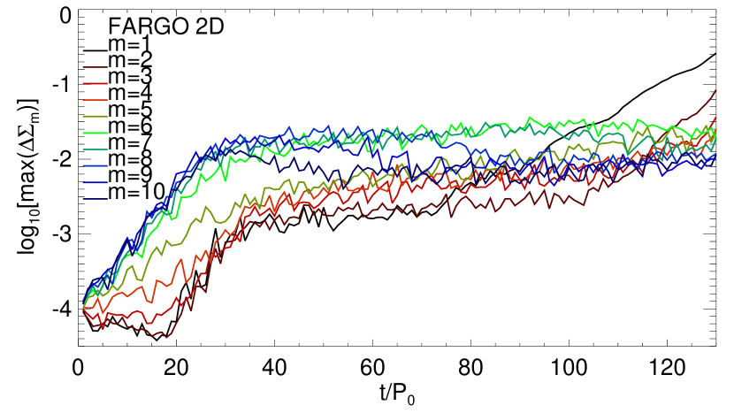
Figure 2: Evolution of non-axisymmetric surface density maxima in the FARGO simulation initialised with perturbations with $m\in[1,10]$.

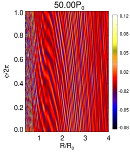
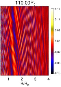
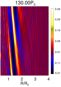
Figure 3: Visualisation of the FARGO 2D simulation in Fig. 2. The total non-axisymmetric surface density $\Delta\Sigma$ is shown.

Fig. 4 shows the evolution of disc angular momentum components. Only the $m=0,\,1$ components are plotted since they are dominant. The $m=1$ structure has an associated negative angular momentum, which indicates it is a low-frequency mode. Its growth is compensated by an increase in the axisymmetric component of angular momentum, such that $\Delta J_{0}+\Delta J_{1}\sim 0$. Note that FARGO does not conserve angular momentum exactly. However, we find the total angular momentum varies by $|\Delta J/J|=O(10^{-6})$, and is much smaller than the change in the angular momenta components, $|\Delta J_{0,1}/J|>O(10^{-5})$. Fig. 4 then suggest that angular momentum is transferred from the one-armed spiral to the background disc.

Figure 4: Evolution of angular momentum components in the FARGO simulation in Fig. 2—3. The perturbation relative to $t=0$ in 2D is shown in units of the initial total angular momentum $J_{\mathrm{ref}}$.

5.2 Dependence on the imposed temperature profile

We show that the growth of the $m=1$ spiral is associated with the imposed temperature gradient by performing a series of simulations with $q\in[0,1]$. However, to maintain similar Toomre $Q$ profiles, we adjust the surface density power-law index such that $s=(3+q)/2$. For clarity these simulations are initialised with $m=1$ perturbations only.

Fig. 5 compares the $m=1$ spiral amplitudes as a function of $q$. We indeed observe slower growth with decreasing $q$. Although the figure indicates growth for the strictly isothermal disc ($q=0$), we did not observe a coherent one-armed spiral upon inspection of the $m=1$ surface density field. The growth in this case may be associated with high-$m$ modes, which dominated the simulation.

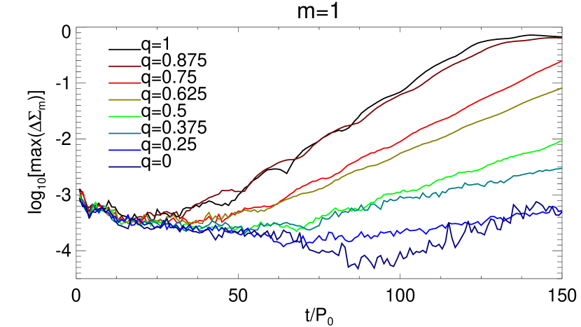
Figure 5: Evolution of the $m=1$ spiral amplitude as a function of the negative of the imposed temperature gradient $q$. The maximum value of the $m=1$ surface density in $R\in[R_{1},R_{2}]$ is shown.

We plot growth rates of the $m=1$ mode as a function of $q$ in Fig. 6. The correlation can be fitted with a linear relation

$$\gamma\simeq\left[0.015q-7.9\times 10^{-4}\right]\Omega_{k}(R_{0}).$$

As the background torque is proportional to $q$ (Eq. 30), this indicates that the temperature gradient is responsible for the development of the one-armed spirals observed in our simulations.

Figure 6: Growth rates of the $m=1$ spiral mode as a function of the imposed sound-speed gradient $q$ (asterisks). A linear fit is also plotted (dotted line).

We also performed a series of simulations with variable aspect-ratio $h\in[0.03,0.07]$ but fixed $q=1$. This affects the magnitude of the temperature gradient since $c_{s}\propto h$. However, with other parameters equal to that in the fiducial simulation, varying $h$ also changes the disc mass. For $h\in[0.03,0.07]$ the total disc mass ranges from $M_{d}=0.052M_{*}$ to $M_{d}=0.12M_{*}$ and the mass within $R\in[R_{1},R_{2}]$ ranges from $0.033M_{*}$ to $0.062M_{*}$.

Fig. 7 shows the growth rates of the $m=1$ spiral in $R\in[R_{1},R_{2}]$ as a function of $h$. Growth rates increases with $h$, roughly as

$$\gamma\simeq\left[0.10h+8.3\times 10^{-3}\right]\Omega_{k}(R_{0}).$$

However, a linear fit is less good than for variable $q$ cases above. This may be due to the change in the total disc mass when $h$ changes. We find no qualitative difference between the spiral pattern that emerges.

Figure 7: Growth rates of the $m=1$ spiral mode as a function of the disc aspect-ratio $h$ (asterisks). A linear fit is also plotted (dotted line).

5.3 Properties of the $m=1$ spiral and its growth

Here we analyse the $q=1$ case in Fig. 6 in more detail.

Fig. 8 shows a snapshot of the $m=1$ surface density of this run. By measuring the $m=1$ surface density amplitude and its pattern speed, we obtain a co-rotation radius and growth rate

$$R_{c}\simeq 4.4R_{0},$$

$$\gamma\simeq 0.014\Omega_{k}(R_{0})=0.13\Omega_{p}.$$

This one-armed spiral can be considered as low frequency because its pattern speed $\Omega_{p}\simeq 0.1\Omega_{k}(R_{0})\;\raisebox{-3.44444pt}{$\buildrel\textstyle<\over{\sim}$}\;0.3\Omega$ in $R\in[R_{1},R_{2}]$ (where it has the largest amplitude). Thus, the spiral pattern appears nearly stationary. The growth rate $\gamma$ is also slow relative to the local rotation, although the characteristic growth time $\gamma^{-1}\simeq 10P_{0}$ is not very long.

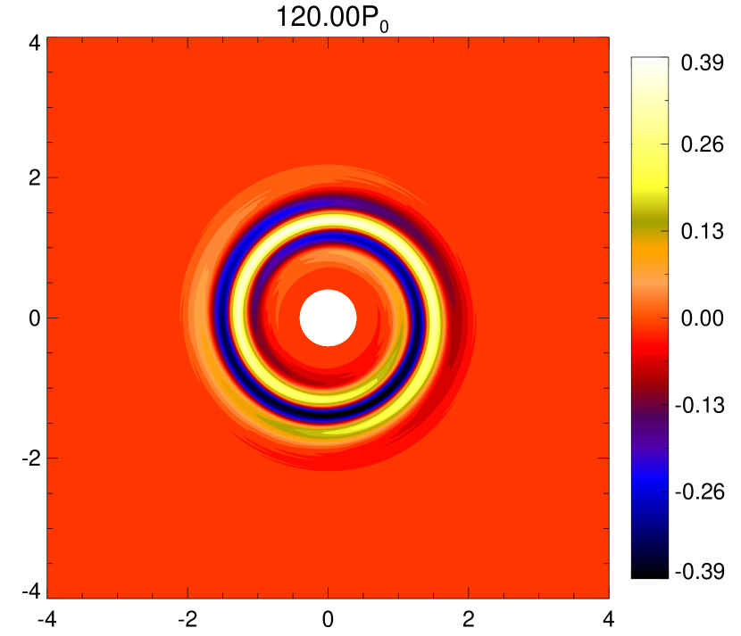
Figure 8: Cartesian visualisation of the $m=1$ surface density structure in the FARGO simulation initialised with only $m=1$ perturbations.

Next, we write $\Sigma_{1}=|\Sigma_{1}|\exp{(\mathrm{i}kR)}$, where $k$ is real, and assume the amplitude $|\Sigma_{1}|$ varies slowly compared to the complex phase. This is the main assumption in local theory. We calculate $k$ numerically and plot its normalised value in Fig. 9. We find

$$kR\sim\frac{\pi G\Sigma}{c_{s}^{2}}R\sim\frac{1}{hQ},$$

where we used $Q\sim c_{s}\Omega/\pi G\Sigma$ and $R\Omega/c_{s}\sim h^{-1}$. Since $Q=O(1)$ and $h\ll 1$ imply $|kR|\gg 1$, we can apply results from local theory (§3.3). Note also that $k\simeq k_{c}$. Fig. 8 shows the $m=1$ spiral is trailing, consistent with $k>0$.

Figure 9: Normalised radial wavenumber of the $m=1$ spiral in Fig. 8.

Using the estimated value of $R_{c}$, we plot in Fig. 10 the quantity $\nu^{2}-1+Q^{-2}$, which is required to be positive in local theory for purely wave-like solutions to the dispersion relation (Eq. 17) when the mode frequency is given. Fig. 10 shows two $Q$-barriers located in the inner disc, at $R_{Qb}=R_{0}$ and $R_{Qb}=1.6R_{0}$; the bounded region is indeed where the $m=1$ spiral develops. This shows that the one-armed spiral is trapped. Note in this region, $\nu^{2}-1+Q^{-2}\simeq 0.1\ll 1$, which is necessary for consistency with the measured wavenumber $k$ and Eq. 18. There is one outer Lindblad resonance at $R_{L}\simeq 7.2R_{0}$. Thus, acoustic waves may be launched in $R\;\raisebox{-3.44444pt}{$\buildrel\textstyle>\over{\sim}$}\;7.2R_{0}$ by the spiral disturbance in the inner disc (Lin & Papaloizou, 2011).

Figure 10: Dimensionless mode frequency $\nu$ for the $m=1$ spiral in Fig. 8. For a given real mode frequency, the dispersion relation for local density waves, Eq. 17, permits purely wave-like solutions in regions where $\nu^{2}-1+Q^{-2}>0$.

We can estimate the expected growth rate of the $m=1$ mode due to the temperature gradient. Setting $k=k_{c}$ and $m=1$ into Eq. 30 gives

$$\gamma\sim\frac{qh}{2Q}\Omega.$$ (47)

Inserting $q=1$, $h=0.05$ and $Q\simeq 1.5$ gives $\gamma\simeq 0.017\Omega$, consistent with numerical results.

5.3.1 Angular momentum exchange with the background disc

We explicitly show that the growth of the $m=1$ spiral is due to the forced temperature gradient via the background torque described in §3. We integrate the statement for angular momentum conservation for linear perturbations, Eq. 13, assuming boundary fluxes are negligible, to obtain

$$\frac{d}{dt}\underbrace{\int_{R_{\mathrm{min}}}^{R_{\mathrm{max}}}j_{\mathrm{lin}}2\pi RdR}_{J_{\mathrm{lin}}}=\int_{R\mathrm{min}}^{R\mathrm{max}}T_{\mathrm{BG}}2\pi RdR,$$ (48)

where we recall $T_{\mathrm{BG}}$ is the torque density associated with the imposed sound-speed profile (Eq. 14). We compute both sides of Eq. 48 using simulation data, and compare them in Fig. 11. There is a good match between the two torques, especially at early times $t\;\raisebox{-3.44444pt}{$\buildrel\textstyle<\over{\sim}$}\;110P_{0}$. The average discrepancy is $\simeq 5\%$. The match is less good later on, when the spiral amplitude is no longer small ($\mathrm{max}\Delta\Sigma_{1}\sim 0.2$ at $t=110P_{0}$ and $\mathrm{max}\Delta\Sigma_{1}\sim 0.4$ by $t=120P_{0}$) and linear theory becomes less applicable. Fig. 11 confirms that the $m=1$ spiral wave experiences a negative torque that further reduces its (negative) angular momentum, leading to its amplitude growth. This is consistent with angular momentum component measurements (Fig. 4).

Figure 11: Rate of change of the $m=1$ wave angular momentum as defined by Eq. 48 (solid) compared to the torque exerted on the wave associated with the background temperature gradient (dotted).

6 Three-dimensional simulations

In this section we review 3D simulations carried out using ZEUS-MP and PLUTO. The main purpose is to verify the above results with different numerical codes, and validate the 2D approximation.

The 3D disc has radial size $[r_{\mathrm{min}},r_{\mathrm{max}}]=[0.4,10]R_{0}$ and vertical extent $n_{H}=2$ scale-heights at $R=R_{0}$. The resolution is $N_{r}\times N_{\theta}\times N_{\phi}=256\times 32\times 512$, or about $4$ cells per $H$. Because of the reduced resolution compared to 2D, we use a smooth perturbation by setting $\delta=10^{-3}$ and $M=1$ in Eq. 46. This corresponds to a single $m=1$ disturbance in $R\in[R_{1},R_{2}]$.

The 3D discs are initialised in approximate equilibrium only, so we first evolve the disc without perturbations using $(l_{\mathrm{max}},m_{\mathrm{max}})=(32,0)$ up to $t=10P_{0}$, during which meridional velocities are damped out. We then restart the simulation with the above perturbation and $(l_{\mathrm{max}},m_{\mathrm{max}})=(32,32)$, and damp meridional velocities near the radial boundaries.

Fig. 12 plots the evolution of the $m=1$ spiral amplitudes measured in the ZEUS-MP and PLUTO runs. We also ran simulations with a strictly isothermal equation of state ($q=0$), which display no growth compared to that with a temperature gradient. This confirms the temperature gradient effect is the same in 3D.

In the ZEUS-MP run, we observed high-$m$ disturbances developed near the inner boundary initially, which is likely responsible for the growth seen at $t<50P_{0}$. This is a numerical artifact and effectively seeds the simulation with a larger perturbation. Results from ZEUS-MP are therefore off-set from PLUTO by $\sim 50P_{0}$. However, once the coherent $m=1$ spiral begins to grow ($t\;\raisebox{-3.44444pt}{$\buildrel\textstyle>\over{\sim}$}\;100P_{0}$), we measure similar growth rates in both codes:

$$\gamma\simeq 0.0073\Omega_{k}(R_{0})\quad\quad\mathrm{PLUTO},$$

$$\gamma\simeq 0.0085\Omega_{k}(R_{0})\quad\quad{\operatorname{ZEUS-MP}}.$$

Both are somewhat smaller than the 2D simulations. This is possibly because of the lower resolutions adopted in 3D and/or because the effective Toomre parameter is larger in 3D (Mamatsashvili & Rice, 2010) which, from Eq. 47, is stabilising.

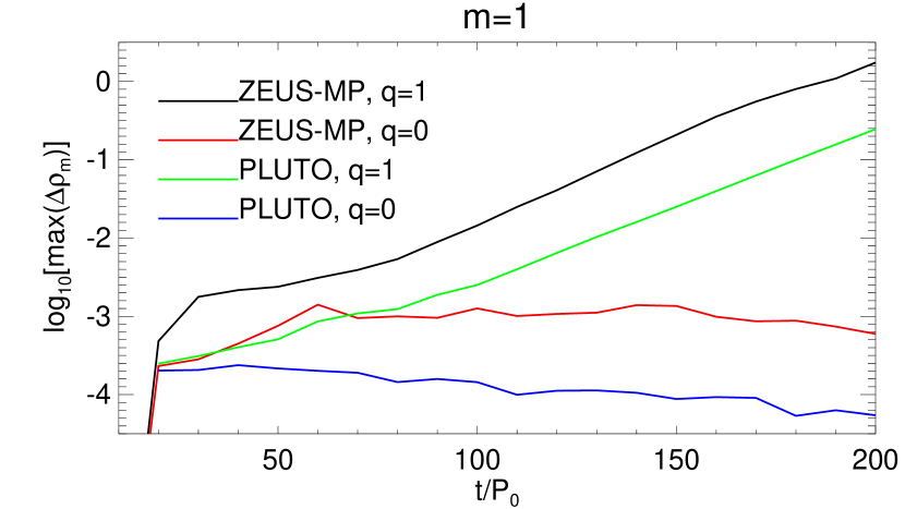
Figure 12: Evolution of the maximum $m=1$ density component in $r\in[R_{1},R_{2}]$ in the 3D simulations. Results from discs with a temperature gradient ($q=1$) and a strictly isothermal disc ($q=0$) are shown.

Visualisations of the 3D simulations are shown in Fig. 13 for the disc midplane and near the upper disc boundary. The snapshots are chosen when the one-armed spirals in the two codes have reached comparable amplitudes. Both codes show similar one-armed patterns at either height, and the midplane snapshot is similar to the 2D simulation (Fig. 3). The largest spiral amplitude is found in the self-gravitating region $R\in[R_{1},R_{2}]$, independent of height. However, notice the spiral pattern extends into the non-self-gravitating outer disc ($R>R_{2}$) at $z\sim 2H$, i.e. the disturbance becomes more global away from the midplane.

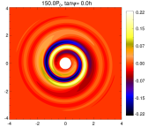
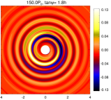
(a) ZEUS-MP

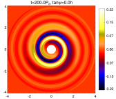
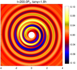
(b) PLUTO

Figure 13: Three-dimensional simulations using the ZEUS-MP (top) and PLUTO (bottom) codes. The $m=1$ density component $\Delta\rho_{1}$ at the midplane (left) and approximately two scale-heights above the midplane (right) is shown. Here $\psi\equiv\pi/2-\theta$ is the angular height from the midplane.

6.1 Vertical structure

Fig. 14 shows the vertical structure of the one-armed spiral in the PLUTO run. The spiral is vertically confined to $z\;\raisebox{-3.44444pt}{$\buildrel\textstyle<\over{\sim}$}\;H$ at $R\sim R_{0}$ (the self-gravitating region). Thus, a 2D disc model, representing dynamics near the disc midplane, is sufficient capture the instability. However, for $R>2R_{0}$ the spiral amplitude increases away from the midplane. It remains small in our disc model ($|\Delta\rho_{1}|\;\raisebox{-3.44444pt}{$\buildrel\textstyle<\over{\sim}$}\;0.1$), but could become significant with a larger vertical domain. This means that 3D simulations are necessary to study the effect of the one-armed spiral on the exterior disc.

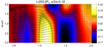
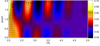
Figure 14: The $m=1$ density component in the meridional plane in the PLUTO simulation. The slices are taken at the azimuth of $\mathrm{max}[\Delta\rho_{1}(r,\pi/2,\phi)]$. Arrows represent the vector $(v_{r}/R_{0},-v_{\theta}/rh\sin^{2}{\theta})$. The top (bottom) panel corresponds to the inner (outer) portions of the disc.

Although Fig. 14 appears to display significant vertical motion, we measure the three-dimensionality parameter $\Theta<10^{-2}$ (Eq. 44), so vertical motions are insignificant compared to horizontal motions. This supports a 2D approximation. On the other hand, we find $\mathrm{max}|v_{z}/c_{s}|\sim 0.2$ which, although sub-sonic, is not very small.

6.2 Angular momentum conservation

Fig. 15 shows the angular momentum evolution in the 3D runs during the linear growth of the one-armed spiral. Because the ZEUS-MP simulation is off-set from PLUTO, the time interval for the plot was chosen such that the change in the angular momentum components are comparable in the two codes.

ZEUS-MP does not conserve angular momentum very well, but the variation in total angular momentum $|\Delta J/J|<O(10^{-6})$ is small compared to the individual components $|\Delta J_{0,1}/J|\sim 10^{-4}$. PLUTO reaches similar values of $|\Delta J_{0,1}|$, but achieves better conservation, with $|\Delta J/J|=O(10^{-8})$. These plots are again similar to the 2D simulations, i.e. angular momentum lost by $J_{1}$ is gained by $J_{0}$. This confirms that the interaction between $J_{1}$ and $J_{0}$ operates in 3D and 2D similarly.

Figure 15: Evolution of angular momentum components in the 3D simulations. The perturbation relative to $t=10P_{0}$, during the growth of the one-armed spiral, is shown in units of the initial total angular momentum $J_{\mathrm{ref}}$.

7 Discussion

We discuss below several issues related to self-gravitating discs in the context of our numerical simulations. However, it is important to keep in mind that the growth of the one-armed spiral in our simulations is not a gravitational instability in the sense that destabilisation is through the background torque associated with a forced temperature gradient, and not by self-gravitational torques.

7.1 Motion of the central star

In our models we have purposefully neglected the indirect potential associated with a non-inertial reference frame to avoid complications arising from the motion of the central star. Although it has been established that such motion can destabilise an $m=1$ disturbance in the disc (Adams, Ruden & Shu, 1989; Shu et al., 1990; Michael & Durisen, 2010), the disc masses in our models ($M_{d}\;\raisebox{-3.44444pt}{$\buildrel\textstyle<\over{\sim}$}\;0.1M_{*}$) are not expected to be sufficiently massive for this effect to be significant. Indeed, simulations including the indirect potential, carried out in the early stages of this project, produced similar results.

7.2 Role of Lindblad and co-rotation torques

One effect of self-gravity is to allow the one-armed spiral, confined to $R\sim R_{0}$ in our models, to act as an external potential for the exterior disc in $R>R_{0}$. This is analogous to disc-satellite interaction (Goldreich & Tremaine, 1979), where the embedded satellite exerts a torque on the disc at Lindblad and co-rotation resonances.

In Appendix C we estimate the magnitude of this effect using basic results from disc-planet theory (see, e.g. Papaloizou et al., 2007, and references therein). There, we find that the angular momentum exchange between the one-armed spiral and the exterior disc is insignificant compared to the background torque.

We confirmed this with additional FARGO simulations that exclude the co-rotation and outer Lindblad resonances (OLR) by reducing radial domain size to $R_{\mathrm{max}}=3R_{0}$, which still developed the one-armed spiral.

7.3 Applicability to protoplanetary discs

7.3.1 Thermodynamic requirements

A locally isothermal equation of state represents the ideal limit of infinitely short cooling and heating timescales, so the disc temperature instantly returns to its initial value when perturbed. The background torque is generally non-zero if the resulting temperature profile has a non-zero radial gradient.

A short cooling timescale $t_{c}$ can occur in the outer parts of protoplanetary discs (Rafikov, 2005; Clarke, 2009; Rice & Armitage, 2009; Cossins, Lodato & Clarke, 2010; Tsukamoto et al., 2015). However, if a disc with $Q\simeq 1$ is cooled (towards zero temperature) on a timescale $t_{c}\;\raisebox{-3.44444pt}{$\buildrel\textstyle<\over{\sim}$}\;\Omega_{k}^{-1}$, it will fragment following gravitational instability (Gammie, 2001; Rice, Lodato & Armitage, 2005; Paardekooper, 2012).

Fragmentation can be avoided if the disc is heated to maintain $Q>Q_{c}$, the threshold for fragmentation ($Q_{c}\simeq 1.4$ for isothermal discs, Mayer et al., 2004). This may be possible in the outer parts of protoplanetary discs due to stellar irradiation (Rafikov, 2009; Kratter & Murray-Clay, 2011; Zhu et al., 2012). Sufficiently strong external irradiation is expected to suppress the linear gravitational instabilities altogether (Rice et al., 2011).

The background torque may thus exist in the outer parts of protoplanetary discs that are irradiated, such that the disc temperature is set externally with a non-zero radial gradient (e.g. Stamatellos & Whitworth, 2008). Of course, if external irradiation sets a strictly isothermal outer disc (e.g. Boley, 2009), then the background torque vanishes.

7.3.2 Radial disc structure

In our simulations the $m=1$ spiral is confined between two $Q$-barriers, where real solutions to the local dispersion relation is possible (Eq. 18). The existence of such a cavity results from the adopted initial surface density bump (Eq. 33). Thus, in our disc models the main role of disc structure and self-gravity is to allow a local $m=1$ mode to be set up, which is then destabilised by the background torque.

In order to confine an $m=1$ mode between two $Q$-barriers, we should have $Q^{2}(1-\nu^{2})=1$ at two radii. Assuming Keplerian rotation and a slow pattern speed $\Omega_{p}\ll\Omega$, this amounts to

$$\left(\frac{R_{Qb}}{R_{c}}\right)^{-3/2}=2Q^{2}(R_{Qb}).$$ (49)

Then two $Q$-barriers may exist when the $Q^{2}$ profile rises more rapidly (decays more slowly) than $R^{-3/2}$ for decreasing (increasing) $R$. Note that Eq. 49 does not necessarily require strong self-gravity if $R_{c}$ is large.

A surface density bump can develop in ‘dead zones’ of protoplanetary discs, where there is reduced mass accretion because the magneto-rotational instability is ineffective for angular momentum transport (Gammie, 1996; Turner & Sano, 2008; Landry et al., 2013). The dead zone becomes self-gravitating with sufficient mass built-up (Armitage, Livio & Pringle, 2001; Martin et al., 2012a, b; Zhu et al., 2009, 2010; Zhu, Hartmann & Gammie, 2010; Bae et al., 2013).

However, conditions in a dead zone may not be suitable for sustaining a background torque because it may not cool/heat fast enough to maintain a fixed temperature profile. Recently, Bae et al. (2014) presented numerical models of dead zones including a range of heating and cooling processes, which show that dead zones developed large-scale (genuine) gravitational instabilities with multiple spiral arms. Although this does not prove absence of the background torque, it is probably insignificant compared to gravitational torques.

Another possibility is a gap opened by an embedded planet. In that case $Q$ rises rapidly towards the gap centre since it is a region of low surface density. This can satisfy Eq. 49. Then the inner edge of our bump function mimics the outer gap edge. The outer gap edge is then a potential site for the growth of a low-frequency one-armed spiral through the background torque. However, the locally isothermal requirement would limit this process to the outer disc, or that the temperature profile about the gap edge is set by the planet luminosity.

Here, it is worth mentioning the transition disc around HD 142527, the outer parts of which displays an $m=1$ asymmetry (Fukagawa et al., 2013) and spiral arms (Christiaens et al., 2014) just outside a disc gap. These authors estimate $Q\simeq$1—2 in the outer disc, implying self-gravity is important, but the disc may remain gravitationally-stable (Christiaens et al., 2014). This is a possible situation that our disc models represent.

8 Summary and conclusions

In this paper, we have described a destabilising effect of adopting a fixed temperature profile to model astrophysical discs. By applying angular momentum conservation within linear theory, we showed that a forced temperature gradient introduces a torque on linear perturbations. We call this the background torque because it represents an exchange of angular momentum between the background disc and the perturbations. This offers a previously unexplored pathway to instability in locally isothermal discs.

In the local approximation, we showed that this background torque is negative for non-axisymmetric trailing waves in discs with a fixed temperature or sound-speed profile that decrease outwards. A negative background torque enforces low-frequency non-axisymmetric modes because they are associated with negative angular momentum.

We demonstrated the destabilising effect of the background torque by carrying out direct numerical hydrodynamic simulations of locally isothermal discs with a self-gravitating surface density bump. We find such systems are unstable to low-frequency perturbations with azimuthal wavenumber $m=1$, which leads to the development of an one-armed trailing spiral that persist for at least $O(10^{2})$ orbits. The spiral pattern speed is smaller than the local disc rotation and growth rates are $O(10^{-2}\Omega)$ which gives a characteristic growth time of $O(10)$ orbits.

We used three independent numerical codes — FARGO in 2D, ZEUS-MP and PLUTO in 3D — to show that the growth of one-armed spirals in our disc model is due to the imposed temperature gradient: growth rates increased linearly with the magnitude of the imposed temperature gradient, and one-armed spirals did not develop in strictly isothermal simulations. This one-armed spiral instability can be interpreted as an initially neutral, tightly-wound $m=1$ mode being destabilised by the background torque. The spiral is mostly confined between two $Q$-barriers in the surface density bump. We find the instability behaves similarly in 2D and 3D, but in 3D the spiral disturbance becomes more radially global away from the midplane.

8.1 Speculations and future work

There are several issues that remain to be addressed in future works:

Thermal relaxation. The locally isothermal assumption can be relaxed by including an energy equation with a source term that restores the disc temperature over a characteristic timescale $t_{\mathrm{relax}}$. Preliminary FARGO simulations indicate a thermal relaxation timescale $t_{\mathrm{relax}}<0.1\Omega_{k}^{-1}$ is needed for the one-armed spiral to develop. However, this value is likely model-dependent. For example, a longer $t_{\mathrm{relax}}$ may be permitted with larger temperature gradients. This issue, together with a parameter survey, will be considered in a follow-up study.

Non-linear evolution. In the deeply non-linear regime, the one-armed spiral may shock and deposit negative angular momentum onto the background disc. The spiral amplitude would saturate by gaining positive angular momentum. However, if the temperature gradient is maintained, it may be possible to achieve a balance between the gain of negative angular momentum through the background torque, and the gain of positive angular momentum through shock dissipation. We remark that fragmentation is unlikely because the co-rotation radius is outside the bulk of the spiral arm (Durisen, Hartquist & Pickett, 2008; Rogers & Wadsley, 2012). In order to study these possibilities, improved numerical models are needed to ensure total angular momentum conservation on timescales much longer than that considered in this paper.

Other applications of the background torque. The background torque is a generic feature in discs for which the temperature is set externally. It may therefore be relevant in other astrophysical contexts. One possibility is in Be star discs (Rivinius, Carciofi & Martayan, 2013), for which one-armed oscillations may explain long-timescale variations in their emission lines (see e.g. Okazaki, 1997; Papaloizou & Savonije, 2006; Ogilvie, 2008, and references therein). These studies invoke alternative mechanisms to produce neutral one-armed oscillations (e.g. rotational deformation of the star), but consider strictly isothermal discs. It would be interesting to explore the effect of a radial temperature gradient on the stability of these oscillations.

Appendix A The background torque density in a three-dimensional disc with a fixed temperature profile

We give a brief derivation of the angular momentum exchange between linear perturbations and the background disc. We consider a three-dimensional disc in which the equilibrium pressure and density are related by

$$p=c_{s}^{2}(R,z)F(\rho),$$ (50)

where $F(\rho)$ is an arbitrary function of $\rho$ with dimensions of mass per unit volume, and $c_{s}$ is a prescribed function of position with dimensions of velocity squared. The equilibrium disc satisfies

$$R\Omega^{2}(R,z) =\frac{1}{\rho}\frac{\partial p}{dR}+\frac{\partial\Phi_{\mathrm{tot}}}{\partial R},$$ (51)

$$0 =\frac{1}{\rho}\frac{\partial p}{\partial z}+\frac{\partial\Phi_{\mathrm{tot}}}{\partial z}.$$ (52)

Note that, in general, the equilibrium rotation $\Omega$ depends on $R$ and $z$.

We begin with the linearised equation of motion in terms of the Lagrangian displacement $\bm{\xi}$ as given by Lin, Papaloizou & Kley (1993) but with an additional potential perturbation,

$$\frac{D^{2}\bm{\xi}}{Dt^{2}}+2\Omega\hat{\bm{z}}\times\frac{D\bm{\xi}}{Dt}$$

$$=-\frac{\nabla\delta p}{\rho}+\frac{\delta\rho}{\rho^{2}}\nabla p-\nabla\delta\Phi_{d}-R\hat{\bm{R}}\left(\bm{\xi}\cdot\nabla\Omega^{2}\right)$$

$$=-\nabla\left(\frac{\delta p}{\rho}+\delta\Phi_{d}\right)-\frac{\delta p}{\rho}\frac{\nabla\rho}{\rho}+\frac{\delta\rho}{\rho}\frac{\nabla p}{\rho}-R\hat{\bm{R}}\left(\bm{\xi}\cdot\nabla\Omega^{2}\right),$$ (53)

where $D/Dt\equiv\partial_{t}+\mathrm{i}m\Omega$ for perturbations with azimuthal dependence in the form $\exp\left(\mathrm{i}m\phi\right)$, and the $\delta$ quantities denote Eulerian perturbations.

As explained in Lin & Papaloizou (2011), a conservation law for the angular momentum of the perturbation may be obtained by taking the dot product between Eq. A and $(-m/2)\rho\bm{\xi}^{*}$, then taking the imaginary part afterwards. The left hand side becomes the rate of change of angular momentum density. The first term on the right hand side (RHS) becomes

$$-\frac{m}{2}\operatorname{Im}\left[-\rho\bm{\xi}^{*}\cdot\nabla\left(\frac{\delta p}{\rho}+\delta\Phi_{d}\right)\right]$$

$$=\frac{m}{2}\operatorname{Im}\left\{\nabla\cdot\left[\rho\bm{\xi}^{*}\left(\frac{\delta p}{\rho}+\delta\Phi_{d}\right)+\frac{1}{4\pi G}\delta\Phi_{d}\nabla\delta\Phi_{d}^{*}\right]\right\}$$

$$+\frac{m}{2}\operatorname{Im}\left(\delta\rho^{*}\frac{\delta p}{\rho}\right),$$ (54)

where $\delta\rho=-\nabla\cdot\left(\rho\bm{\xi}\right)$ and $\nabla^{2}\delta\Phi_{d}=4\pi G\delta\rho$ have been used. The terms in square brackets on the RHS of Eq. A is (minus) the angular momentum flux. The second term on RHS of Eq. A, together with the remaining terms on the RHS of Eq. A constitutes the background torque. That is,

$$T_{\mathrm{BG}}=\frac{m}{2}\operatorname{Im}\left[\frac{\delta p}{\rho}\Delta\rho^{*}-\frac{\delta\rho}{\rho}\bm{\xi}^{*}\cdot\nabla p+\rho\xi_{R}^{*}\xi_{z}\frac{\partial\left(R\Omega^{2}\right)}{\partial z}\right],$$ (55)

where $\Delta\rho=\delta\rho+\bm{\xi}\cdot\nabla\rho$ is the Lagrangian density perturbation.

So far we have not invoked an energy equation. For adiabatic perturbations $T_{\mathrm{BG}}$ is zero, and we recover the same statement of angular momentum conservation as in Lin, Papaloizou & Kley (1993) but modified by self-gravity in the fluxes.

However, if we impose the equilibrium relation Eq. 50 to hold in the perturbed state, then

$$\delta p=c_{s}^{2}(R,z)F^{\prime}\delta\rho,$$ (56)

where $F^{\prime}=dF/d\rho$. Inserting this into Eq. 55, we obtain

$$T_{\mathrm{BG}}=-\frac{m}{2}\frac{p}{\rho c_{s}^{2}}\operatorname{Im}\left[\delta\rho\bm{\xi}^{*}\cdot\nabla c_{s}^{2}+\xi_{R}^{*}\xi_{z}\left(\frac{\partial\rho}{\partial z}\frac{\partial c_{s}^{2}}{\partial R}-\frac{\partial\rho}{\partial R}\frac{\partial c_{s}^{2}}{\partial z}\right)\right],$$ (57)

where the equilibrium equations were used. At this point setting $\xi_{z}=0$ gives $T_{\mathrm{BG}}$ for perturbations with no vertical motion,

$$T_{\mathrm{BG,2D}}=-\frac{m}{2}\frac{p}{\rho c_{s}^{2}}\operatorname{Im}\left(\delta\rho\xi_{R}^{*}\partial_{R}c_{s}^{2}\right),$$ (58)

and is equivalent to the 2D expression, Eq. 14, with $\delta\rho$ replaced by $\delta\Sigma$ and $p=c_{s}^{2}\rho$.

In fact, we can simplify Eq. 57 in the general case by using $\delta\rho=-\rho\nabla\cdot\bm{\xi}-\bm{\xi}\cdot\nabla\rho$, giving

$$T_{\mathrm{BG}}=\frac{m}{2}\frac{p}{\rho c_{s}^{2}}\operatorname{Im}\left[\rho\left(\nabla\cdot\bm{\xi}\right)\bm{\xi}^{*}\cdot\nabla c_{s}^{2}\right].$$ (59)

For a barotropic fluid $p=p(\rho)$, the function $c_{s}^{2}$ can be taken as constant (Eq. 50) for which $T_{\mathrm{BG}}$ vanishes. When there is a forced temperature gradient, Eq. 59 indicates a torque is applied to compressible perturbations ($\nabla\cdot\bm{\xi}\neq 0$) if there is motion along the temperature gradient ($\bm{\xi}\cdot\nabla c_{s}^{2}\neq 0$).

Appendix B Relation between horizontal Lagrangian displacements for local, low frequency disturbances

Here, we aim to relate the horizontal Lagrangian displacements $\xi_{R}$ and $\xi_{\phi}$ in the local approximation. Using the local solution to the Poisson equation

$$\delta\Phi_{m}=-\frac{2\pi G}{|k|}\delta\Sigma_{m}$$ (60)

(Shu, 1991), the linearised azimuthal equation of motion becomes

$$-\mathrm{i}\bar{\sigma}\delta v_{\phi m}+\frac{\kappa^{2}}{2\Omega}\delta v_{Rm}=-\frac{\mathrm{i}m}{R\Sigma}\left(c_{s}^{2}-\frac{2\pi G\Sigma}{|k|}\right)\delta\Sigma_{m}.$$ (61)

Next, we replace the surface density perturbation $\delta\Sigma_{m}=-\mathrm{i}k\Sigma\xi_{R}$, and use the expressions

$$\delta v_{Rm}=-\mathrm{i}\bar{\sigma}\xi_{R},$$ (62)

$$\delta v_{\phi m}=-\mathrm{i}\bar{\sigma}\xi_{\phi}-\frac{\mathrm{i}R\partial_{R}\Omega}{\bar{\sigma}}\delta v_{Rm}$$ (63)

(Papaloizou & Pringle, 1985) to obtain

$$-\bar{\sigma}^{2}\xi_{\phi}-2\mathrm{i}\bar{\sigma}\Omega\xi_{R}=\frac{m}{kR}\left(\kappa^{2}-\bar{\sigma}^{2}\right)\xi_{R},$$ (64)

where the dispersion relation Eq. 17 was used. In the local approximation, $|kR|\gg m$ by assumption. Hence the RHS of this equation can be neglected. Then

$$\xi_{\phi}\simeq-\frac{2\mathrm{i}\Omega}{\bar{\sigma}}\xi_{R}.$$ (65)

For low-frequency modes we have $\bar{\sigma}\simeq-m\Omega$, so $\xi_{\phi}\simeq 2\mathrm{i}\xi_{R}/m$, as used in the main text.

Appendix C The confined spiral as an external potential

Let us treat the one-armed spiral confined in $R\in[R_{1},R_{2}]$ as an external potential of the form $\Phi_{\mathrm{ext}}(R)\cos{\left(\phi-\Omega_{p}t\right)}$. We take

$$\Phi_{\mathrm{ext}}=-\frac{GM_{\mathrm{ring}}}{\overline{R}}b^{1}_{1/2}(\beta),$$ (66)

where $M_{\mathrm{ring}}$ is the disc mass contained within $R\in[R_{1},R_{2}]$, $\overline{R}=(R_{1}+R_{2})/2$ is the approximate radial location of the spiral, $b_{n}^{m}(\beta)$ is the Laplace coefficient and $\beta=R/\overline{R}$. This form of $\Phi_{\mathrm{ext}}$ is the $m=1$ component of the gravitational potential of an external satellite on a circular orbit (Goldreich & Tremaine, 1979).

We expect the external potential to exert a torque on the disc at the Lindblad and co-rotation resonances. At the outer Lindblad resonance (OLR), this torque is

$$\Gamma_{L}=\frac{\pi^{2}\Sigma_{L}}{3\Omega_{L}\Omega_{p}}\left[\left.R_{L}\frac{d\Phi_{\mathrm{ext}}}{dR}\right|_{L}+2\left(1-\frac{\Omega_{p}}{\Omega_{L}}\right)\Phi_{\mathrm{ext}}\right]^{2},$$ (67)

where a Keplerian disc has been assumed and subscript $L$ denotes evaluation at the OLR, $R=R_{L}$. (The inner Lindblad resonance does not exist for the pattern speeds observed in our simulations.)

If we associate the external potential with an angular momentum magnitude of $J_{\mathrm{ext}}=M_{\mathrm{ring}}\overline{R}^{2}\Omega_{p}$, we can calculate a rate of change of angular momentum $\gamma_{L}=\Gamma_{L}/J_{\mathrm{ext}}$. Then

$$\frac{\gamma_{L}}{\Omega_{p}}= \frac{\pi h}{3Q_{L}}\left(\frac{M_{p}}{M_{*}}\right)\left(\frac{R_{L}}{\overline{R}}\right)\left(\frac{R_{c}}{\overline{R}}\right)^{3}\left(\frac{R_{L}}{R_{c}}\right)^{-3/2}$$

$$\times\left\{\frac{R_{L}}{\overline{R}}\left.\frac{db_{1/2}^{1}}{d\beta}\right|_{L}+2\left[1-\left(\frac{R_{c}}{R_{L}}\right)^{-3/2}\right]b_{1/2}^{1}(\beta_{L})\right\}^{2}.$$ (68)

Inserting $h=0.05$, $Q_{L}=10$, $M_{\mathrm{ring}}=0.05M_{*}$, $R_{L}=7.2R_{0}$, $R_{c}=4.4R_{0}$ and $\overline{R}=1.5R_{0}$ from our fiducial FARGO simulation, we get

$$\gamma_{L}\sim 5\times 10^{-4}\Omega_{p}.$$ (69)

For the co-rotation torque, we use the result

$$\Gamma_{c}=\left.\pi^{2}\Phi_{\mathrm{ext}}^{2}\left(\frac{d\Omega}{dR}\right)^{-1}\frac{d}{dR}\left(\frac{2\Sigma}{\Omega}\right)\right|_{c}$$ (70)

for a Keplerian disc, where subscript $c$ denotes evaluation at co-rotation radius $R=R_{c}$. For a power-law surface density profile $\Sigma\propto R^{-s}$ we have

$$\frac{\gamma_{c}}{\Omega_{p}}=\frac{4}{3}\frac{\pi h}{Q_{c}}\left(\frac{M_{\mathrm{ring}}}{M_{*}}\right)\left(\frac{R_{c}}{\overline{R}}\right)^{4}\left(s-\frac{3}{2}\right)\left[b_{1/2}^{1}(\beta_{c})\right]^{2}$$ (71)

Using the above parameter values with $s=2$ and $Q_{c}=10$, we obtain a rate

$$\gamma_{c}\sim 6\times 10^{-4}\Omega_{p}.$$ (72)

The torque exerted on the disc at the OLR by an external potential is positive, while that at co-rotation depends on the gradient of potential vorticity there (Goldreich & Tremaine, 1979). For our disc models with surface density $\Sigma\propto R^{-2}$ in the outer disc, this co-rotation torque is positive. This means that the one-armed spiral loses angular momentum by launching density waves with positive angular momentum at the OLR, and by applying a positive co-rotation torque on the disc. In principle, this interaction is destabilising because the one-armed spiral has negative angular momentum (Lin & Papaloizou, 2011).

However, the above estimates for $\gamma_{L}$ and $\gamma_{c}$ are much smaller than that due to the imposed temperature gradient as measured in the simulations ($\gamma\sim∼0.1\Omega_{p}$). We conclude that for our disc models, the Lindblad and co-rotation resonances have negligible effects on the growth of the one-armed spiral in the inner disc (but it could be important in other parameter regimes).

References

- Adams, Ruden & Shu (1989) Adams F. C., Ruden S. P., Shu F. H., 1989, ApJ, 347, 959
- Armitage, Livio & Pringle (2001) Armitage P. J., Livio M., Pringle J. E., 2001, MNRAS, 324, 705
- Avenhaus et al. (2014) Avenhaus H., Quanz S. P., Schmid H. M., Meyer M. R., Garufi A., Wolf S., Dominik C., 2014, ApJ, 781, 87
- Bae et al. (2013) Bae J., Hartmann L., Zhu Z., Gammie C., 2013, ApJ, 764, 141
- Bae et al. (2014) Bae J., Hartmann L., Zhu Z., Nelson R. P., 2014, ApJ, 795, 61
- Balbus & Papaloizou (1999) Balbus S. A., Papaloizou J. C. B., 1999, ApJ, 521, 650
- Baruteau et al. (2013) Baruteau C. et al., 2013, ArXiv e-prints
- Baruteau & Masset (2008) Baruteau C., Masset F., 2008, ApJ, 678, 483
- Boccaletti et al. (2013) Boccaletti A., Pantin E., Lagrange A.-M., Augereau J.-C., Meheut H., Quanz S. P., 2013, A&A, 560, A20
- Boley (2009) Boley A. C., 2009, ApJL, 695, L53
- Boss (1980) Boss A. P., 1980, ApJ, 236, 619
- Casassus et al. (2013) Casassus S. et al., 2013, Nature, , 493, 191
- Christiaens et al. (2014) Christiaens V., Casassus S., Perez S., van der Plas G., Ménard F., 2014, ApJL, 785, L12
- Clarke (2009) Clarke C. J., 2009, MNRAS, 396, 1066
- Cossins, Lodato & Clarke (2010) Cossins P., Lodato G., Clarke C., 2010, MNRAS, 401, 2587
- Cossins, Lodato & Testi (2010) Cossins P., Lodato G., Testi L., 2010, MNRAS, 407, 181
- Dipierro et al. (2014) Dipierro G., Lodato G., Testi L., de Gregorio Monsalvo I., 2014, MNRAS, 444, 1919
- Durisen, Hartquist & Pickett (2008) Durisen R. H., Hartquist T. W., Pickett M. K., 2008, ApSS, 317, 3
- Follette et al. (2014) Follette K. B. et al., 2014, ArXiv e-prints
- Forgan et al. (2011) Forgan D., Rice K., Cossins P., Lodato G., 2011, MNRAS, 410, 994
- Fukagawa et al. (2013) Fukagawa M. et al., 2013, PASJ, 65, L14
- Gammie (1996) Gammie C. F., 1996, ApJ, 457, 355
- Gammie (2001) Gammie C. F., 2001, ApJ, 553, 174
- Goldreich & Lynden-Bell (1965) Goldreich P., Lynden-Bell D., 1965, MNRAS, 130, 125
- Goldreich & Tremaine (1979) Goldreich P., Tremaine S., 1979, ApJ, 233, 857
- Grady et al. (2013) Grady C. A. et al., 2013, ApJ, 762, 48
- Hashimoto et al. (2011) Hashimoto J. et al., 2011, ApJL, 729, L17
- Hayes et al. (2006) Hayes J. C., Norman M. L., Fiedler R. A., Bordner J. O., Li P. S., Clark S. E., ud-Doula A., Mac Low M., 2006, ApJS, , 165, 188
- Heemskerk, Papaloizou & Savonije (1992) Heemskerk M. H. M., Papaloizou J. C., Savonije G. J., 1992, A&A, 260, 161
- Hopkins (2010) Hopkins P. F., 2010, ArXiv e-prints
- Inutsuka, Machida & Matsumoto (2010) Inutsuka S.-i., Machida M. N., Matsumoto T., 2010, ApJL, 718, L58
- Isella et al. (2013) Isella A., Pérez L. M., Carpenter J. M., Ricci L., Andrews S., Rosenfeld K., 2013, ApJ, 775, 30
- Juhasz et al. (2014) Juhasz A., Benisty M., Pohl A., Dullemond C., Dominik C., Paardekooper S.-J., 2014, ArXiv e-prints
- Kimura & Tsuribe (2012) Kimura S. S., Tsuribe T., 2012, PASJ, 64, 116
- Kratter et al. (2010) Kratter K. M., Matzner C. D., Krumholz M. R., Klein R. I., 2010, ApJ, 708, 1585
- Kratter & Murray-Clay (2011) Kratter K. M., Murray-Clay R. A., 2011, ApJ, 740, 1
- Landry et al. (2013) Landry R., Dodson-Robinson S. E., Turner N. J., Abram G., 2013, ApJ, 771, 80
- Laughlin & Korchagin (1996) Laughlin G., Korchagin V., 1996, ApJ, 460, 855
- Laughlin, Korchagin & Adams (1997) Laughlin G., Korchagin V., Adams F. C., 1997, ApJ, 477, 410
- Laughlin, Korchagin & Adams (1998) Laughlin G., Korchagin V., Adams F. C., 1998, ApJ, 504, 945
- Laughlin & Rozyczka (1996) Laughlin G., Rozyczka M., 1996, ApJ, 456, 279
- Lin, Papaloizou & Kley (1993) Lin D. N. C., Papaloizou J. C. B., Kley W., 1993, ApJ, 416, 689
- Lin (2012) Lin M.-K., 2012, MNRAS, 426, 3211
- Lin (2014) Lin M.-K., 2014, MNRAS, 437, 575
- Lin & Cloutier (2014) Lin M.-K., Cloutier R., 2014, in IAU Symposium, Vol. 299, IAU Symposium, Booth M., Matthews B. C., Graham J. R., eds., pp. 218–219
- Lin & Papaloizou (2011) Lin M.-K., Papaloizou J. C. B., 2011, MNRAS, 415, 1445
- Lodato & Rice (2004) Lodato G., Rice W. K. M., 2004, MNRAS, 351, 630
- Lodato & Rice (2005) Lodato G., Rice W. K. M., 2005, MNRAS, 358, 1489
- Lynden-Bell & Kalnajs (1972) Lynden-Bell D., Kalnajs A. J., 1972, MNRAS, 157, 1
- Mamatsashvili & Rice (2010) Mamatsashvili G. R., Rice W. K. M., 2010, MNRAS, 406, 2050
- Martin et al. (2012a) Martin R. G., Lubow S. H., Livio M., Pringle J. E., 2012a, MNRAS, 420, 3139
- Martin et al. (2012b) Martin R. G., Lubow S. H., Livio M., Pringle J. E., 2012b, MNRAS, 423, 2718
- Masset (2000a) Masset F., 2000a, A&AS, , 141, 165
- Masset (2000b) Masset F. S., 2000b, in Astronomical Society of the Pacific Conference Series, Vol. 219, Disks, Planetesimals, and Planets, Garzón G., Eiroa C., de Winter D., Mahoney T. J., eds., pp. 75–+
- Matzner & Levin (2005) Matzner C. D., Levin Y., 2005, ApJ, 628, 817
- Mayer et al. (2004) Mayer L., Quinn T., Wadsley J., Stadel J., 2004, ApJ, 609, 1045
- Michael & Durisen (2010) Michael S., Durisen R. H., 2010, MNRAS, 406, 279
- Mignone et al. (2007) Mignone A., Bodo G., Massaglia S., Matsakos T., Tesileanu O., Zanni C., Ferrari A., 2007, ApJS, , 170, 228
- Müller, Kley & Meru (2012) Müller T. W. A., Kley W., Meru F., 2012, A&A, 541, A123
- Muto et al. (2012) Muto T. et al., 2012, ApJL, 748, L22
- Narayan, Goldreich & Goodman (1987) Narayan R., Goldreich P., Goodman J., 1987, MNRAS, 228, 1
- Nelson et al. (1998) Nelson A. F., Benz W., Adams F. C., Arnett D., 1998, ApJ, 502, 342
- Ogilvie (2008) Ogilvie G. I., 2008, MNRAS, 388, 1372
- Okazaki (1997) Okazaki A. T., 1997, A&A, 318, 548
- Paardekooper (2012) Paardekooper S.-J., 2012, MNRAS, 421, 3286
- Papaloizou & Savonije (1991) Papaloizou J. C., Savonije G. J., 1991, MNRAS, 248, 353
- Papaloizou (2002) Papaloizou J. C. B., 2002, A&A, 388, 615
- Papaloizou et al. (2007) Papaloizou J. C. B., Nelson R. P., Kley W., Masset F. S., Artymowicz P., 2007, in Protostars and Planets V, Reipurth B., Jewitt D., Keil K., eds., pp. 655–668