The Metal-Enriched Thermal Composite Supernova Remnant Kesteven 41 (G337.8–0.1) in a Molecular Environment

Abstract

The physical nature of thermal composite supernova remnants (SNRs) remains controversial. We have revisited the archival XMM-Newton and Chandra data of the thermal composite SNR Kesteven 41 (Kes 41 or G337.8$-$0.1) and performed a millimeter observation towards this source in ${}^{12}{\rm CO}$, ${}^{13}{\rm CO}$, and ${\rm C}^{18}{\rm O}$ lines. The X-ray emission, mainly concentrated toward the southwestern part of the SNR, is characterized by distinct S and Ar He-like lines in the spectra. The X-ray spectra can be fitted with an absorbed non-equilibrium ionization collisional plasma model at a temperature 1.3–2.6 keV and an ionization timescale $0.1$–$1.2\times 10^{12}\,{\rm cm}^{-3}\,{\rm s}$. The metal species S and Ar are over-abundant, with 1.2–2.7 and 1.3–3.8 solar abundances, respectively, which strongly indicate the presence of a substantial ejecta component in the X-ray emitting plasma of this SNR. Kes 41 is found to be associated with a giant molecular cloud (MC) at a systemic LSR velocity $-50\,{\rm km}\,{\rm s}^{-1}$ and confined in a cavity, delineated by a northern molecular shell, a western concave MC that features a discernible shell, and an H I cloud seen toward the southeast of the SNR. The birth of the SNR in a pre-existing molecular cavity implies a mass $\gtrsim 18M_{\odot}$ for the progenitor if it was not in a binary system. Thermal conduction and cloudlet evaporation seem to be feasible mechanisms to interpret the X-ray thermal composite morphology, while the scenario of gas-reheating by the shock reflected from the cavity wall is quantitatively consistent with the observations. An updated list of thermal composite SNRs is also presented in this paper.

1 Introduction

Massive stars rapidly evolve to the end of their nuclear-burning lifetimes and explode as core-collapse (CC) supernovae before they can move far away from where they formed. Dozens of CC supernova remnants (SNRs) have been found to be interacting with molecular clouds (MCs) (see Jiang et al., 2010, and references therein). Such SNRs are a crucial probe for hadronic interactions between the shock accelerated protons and the associated MCs, and many detections of them have been made based on $\gamma$-ray observations in the current Fermi and HESS era. Among them are a number of so-called thermal composite (Jones et al., 1998; Wilner et al., 1998) or mixed-morphology remnants (Rho & Petre, 1998); this class of SNRs is characterized by the coexistence of radio shells and centrally brightened thermal X-ray emission. The large majority of thermal composite SNRs have been found to be interacting with adjacent MCs (Green et al., 1997; Yusef-Zadeh et al., 2003). Unlike the regular composite type SNRs in which the central X-ray emission is clearly known to be powered by pulsars, the nature of the X-ray kernel in the thermal composites remains a controversial issue.

Several attempts have been made to interpret the X-ray morphology of the thermal composites and some mechanisms to explain the center-filled X-ray morphology have been proposed, including hot interior with radiatively cooled rim, thermal conduction in the interior hot gas, gas evaporation from the shock-engulfed cloudlets, projection effects of the one-sided shock-cloud interaction, metal enrichment in the interior, shock reflected inward from wind-blown cavity wall, amonst other proposed mechanisms (see a summary in Chen et al., 2008, and references therein). More studies of thermal composite SNRs are needed to test these mechanisms. For this purpose, we here investigate the properties of the interior hot gas and the environs of SNR Kesteven 41 (Kes 41 for the remainder of this paper).

Kes 41 (G337.8$-$0.1), a southern-sky SNR first discovered with the Molonglo Observatory Synthesis telescope (MOST) at 408$\,{\rm MHz}$ (Shaver & Goss, 1970), is shown to be centrally brightened in X-rays within a distorted radio shell by an XMM-Newton observation and is therefore classified as a thermal composite SNR (Combi et al., 2008). In a spectral analysis, the X-ray emission was suggested to arise from a hot ($\sim 1.4\,{\rm keV}$) gas of normal metal abundance; however, only the MOS data of the XMM-Newton have been analyzed so far (Combi et al., 2008). Presently, the available X-ray observations allow a more thorough analysis of the physical properties of Kes 41.

Moreover, Kes 41 has been found to be interacting with an adjacent MC as indicated by the 1720$\,{\rm MHz}$ hydroxyl radical (OH) maser emission detected on the radio shell (Koralesky et al., 1998; Caswell, 2004). The OH satellite line masers at 1720$\,{\rm MHz}$ are widely accepted as a signpost of SNR-MC interaction (Lockett et al., 1999; Frail & Mitchell, 1998; Wardle & Yusef-Zadeh, 2002). The SNR-MC interaction may probably contribute to the high-energy $\gamma$-ray excess near Kes 41 detected by EGRET (Casandjian & Grenier, 2008) and Fermi (Ergin & Ercan, 2012) satellites. The distance to the remnant is estimated to be 12.3$\,{\rm kpc}$ from the OH maser detection at the local standard of rest (LSR) velocity $-45\,{\,{\rm km}\,{\rm s}^{-1}}$ (Koralesky et al., 1998) and the H I absorption that places it beyond the tangent point at 7.9$\,{\rm kpc}$ (Caswell et al., 1975). As a follow-up study of the association of Kes 41 with an adjacent MC, we have performed a millimeter observation toward Kes 41 of CO transition lines.

In this paper we carry out an X-ray analysis of SNR Kes 41 with archival XMM-Newton (MOS and PN) and Chandra observation data and investigate the ambient interstellar environment with our new CO line observation as well as an archival H I survey.

2 Observations and Data Reduction

2.1 XMM-Newton and Chandra X-ray Observations

The XMM-Newton X-ray satellite observed Kes 41 on September 26th 2005 using both the EPIC-MOS and the EPIC-PN (Combi et al., 2008), centered at (RA (J2000.0) $={16}^{{\rm h}}{39}^{{\rm m}}{06}\fs 5$, DEC (J2000.0) $={-46}^{\circ}{57}^{\prime}{58}\farcs 0$). The raw EPIC data are cleaned with the latest version of the Standard Analysis System (SAS-V13.0.3), of which the Extended Source Analysis Software (ESAS) package is mainly used because Kes 41 appears as an extended source in these observations. After removing time intervals with heavy proton flarings, the effective net exposure time for both the EPIC-MOS and the EPIC-PN is 35$\,{\rm ksec}$. We exclude flux from all the detected point sources before performing spatial and spectral analyses.

Chandra observed Kes 41 with the Advanced CCD Imaging Spectrometer (ACIS) on June 2011 incidentally in an observation towards high-mass X-ray binaries in the Norma region (PI: John Tomsick). There are six sections of the observation that cover Kes 41 region (see Table 1 for observational parameters). We reprocess the events files using the Chandra Interactive Analysis of Observations (CIAO) data processing software (Version 4.5). In the reprocessing, bad grades are filtered out and good time intervals are reserved. Flux from all the detected point sources in the field of view (FOV) are also removed.

2.2 CO Observation and Data

The spectroscopic mapping observation of CO molecular lines, i.e. ${}^{12}{\rm CO}$ ($J$=1–0) at 115.271$\,{\rm GHz}$, ${}^{13}{\rm CO}$ ($J$=1–0) at 110.201$\,{\rm GHz}$, and ${\rm C}^{18}{\rm O}$ ($J$=1–0) at 109.782$\,{\rm GHz}$, was made with the Mopra 22-m telescope in Australia on 7–11 July 2011. We did on-the-fly (OTF) mapping with the field of $\sim 11^{\prime}\times 10^{\prime}$ covering the entire angular extent of Kes 41. The 3-mm band receiver and the Mopra spectrometer backend system were used in zoom mode. The bandwidth in this mode is about 137.5$\,{\rm MHz}$ (corresponding to about 360$\,{\rm km}\,{\rm s}^{-1}$ for ${}^{12}{\rm CO}$ ($J$=1–0)) with a spectral resolution of about 33.6$\,{\rm kHz}$ (corresponding to an LSR velocity resolution of $\sim 0.09\,{\rm km}\,{\rm s}^{-1}$). During the observation the system temperature was around 280 K and the pointing accuracy was mostly better than $\sim 3.5^{\prime\prime}$. The half-power beam size is $\sim 30^{\prime\prime}$ at 115$\,{\rm GHz}$, with the main beam efficiency $\sim 0.42$ at the same wave band (Ladd et al., 2005). In this paper, all the images are presented in antenna temperature, but radiative temperature after calibration is used to derive the physical parameters of the molecular gas.

The software Livedata/Gridzilla is used to calibrate the OTF-mapping data and combine them into three-dimensional data cubes, with two spatial dimensions (longitude/latitude) and one spectral dimension (LSR velocity). The subsequent data reduction, such as subtracting fitted polynomial baselines, are performed using our own script written in Python. Three data cubes of diverse CO lines are yielded with grid spacing of $30^{\prime\prime}$ and velocity resolution of $\sim 0.1\,{\,{\rm km}\,{\rm s}^{-1}}$. Finally, the mean rms noise levels of the main beam brightness temperature are about 0.3, 0.15, and 0.15 K for the ${}^{12}{\rm CO}$ ($J$=1–0), ${}^{13}{\rm CO}$ ($J$=1–0), and ${\rm C}^{18}{\rm O}$ ($J$=1–0) lines respectively.

2.3 Other data

The archival radio data from the MOST Galactic plane survey at $843\,{\rm MHz}$ (with an angular resolution of $\sim 43^{\prime\prime}$; Whiteoak & Green, 1996), and the SGPS H I data (with an angular resolution of $\sim 2^{\prime}$ and a spectral resolution of $\sim 0.8\,{\rm km}\,{\rm s}^{-1}$; McClure-Griffiths et al., 2005) are also used in our multi-wavelength study of Kes 41.

3 Analyses and Results

3.1 X-ray properties

3.1.1 Spatial analysis

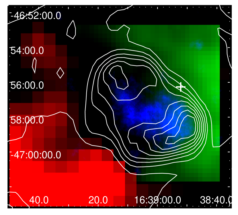
Figure 1: Tricolor image of Kes 41 in multiwavelength. Blue: XMM-Newton X-ray image (2.0–7.2$\,{\rm keV}$) obtained by combining the EPIC-PN and MOS data. Green: ${}^{12}{\rm CO}$ ($J$=1–0) integrated map ($V_{\scriptscriptstyle\rm LSR}=-70$– $-40\,{\,{\rm km}\,{\rm s}^{-1}}$). Red: H I line emission from SGPS integrated map ($V_{\scriptscriptstyle\rm LSR}=-55$– $-50\,{\,{\rm km}\,{\rm s}^{-1}}$). The image is overlaid with MOST 843$\,{\rm MHz}$ radio contours (at seven linear scale levels between 0.00 and 0.79$\,{\rm Jy}\,{\rm beam}^{-1}$; from Whiteoak & Green (1996)). The white cross indicates the location of $1720\,{\rm MHz}$ OH maser (Koralesky et al., 1998) in this SNR.

In Figure 1 we present a broadband (2.0–7.2  keV) X-ray image of Kes 41 made from the EPIC-MOS and EPIC-PN data, as coded in blue. In this image, we have removed the bad pixels, masked the detected point sources for both MOS and PN, merged the MOS and PN imaging data with the quiescent particle background subtracted and exposure map correction applied, and adaptively smoothed the image (using the tool fadapt of HEASOFT, version 6.14). It can be clearly seen that the X-ray emission is internally filled without limb brightening as contrasted to the shell-like feature in radio (shown in white contours). The centroid of the X-ray emission sits in the southwest (SW) region of the northeast-southwest elongated extent of the SNR.

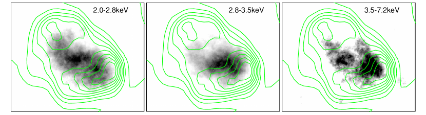
Figure 2: The XMM-Newton (MOS+PN) X-ray images of Kes 41 in energy bands 2.0-2.8$\,{\rm keV}$, 2.8-3.5$\,{\rm keV}$, and 3.5-7.2$\,{\rm keV}$, with radio contours (the same as in Figure 1) overlaid.

In Figure 2 we present X-ray images that are produced in the 2.0–2.8  keV, 2.8–3.5  keV and 3.5–7.2  keV energy ranges, respectively, following the similar procedure for the broad band image. These images illustrate the photon energy dependence for broadband intensities. The narrow bands correspond to the sulfur line, argon line (see § 3.1.2), and higher energy emission, respectively. In both the soft (2.0–2.8 keV) and hard (3.5–7.2 keV) images, there are two X-ray brightness peaks located in the geometric center and the southwestern region. The hard X-ray image looks relatively bright in the SW compared with that in the NE.

All six short sections of the Chandra observation described in Table 1 are also used to generate a merged broadband image of Kes 41, but the location of SNR is near to the edge of the CCD chips in each section of observation, resulting in a decrease of the angular resolution. The Chandra X-ray image of the SNR shows no significant difference from the XMM-Newton image and is not presented here.

3.1.2 Spectral analysis

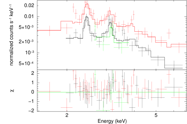
Figure 3: X-ray spectra of the region defined in Figure 4 from both XMM-Newton and Chandra observations. Red points show the EPIC-PN data; the black points are from the merged EPIC-MOS1/2 data; the green points show the co-added spectrum made by merging all 3 Chandra observations that cover the majority of the SNR’s X-ray emission as described in Section 3.1.2. All the spectra have been adaptively binned to achieve a background-subtracted S/N (signal-to-noise ratio) of 3 per bin. They are jointly fitted using the same absorbed vnei model and the lines with different colors are fitted model lines matching the same color data points separately.

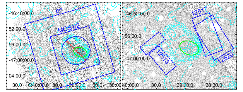
Figure 4: Raw images of the XMM-Newton observation (left) and merged Chandra observations (right), with all detected point sources removed. The common ellipse (in green) is used for source spectral extraction. In the left panel, the dashed boxes, excluding the dashed circle with the crossing line (in red), are used for PN and MOS1/MOS2 background subtraction. In the right panel, the boxes with the numbers denoting the Obs. IDs in Table 1 are used as background regions for the corresponding data. The cyan contours are from radio observation, with levels the same as in Figure 1.

Figure 3 shows the simultaneous fit of the XMM-Newton and Chandra spectra of Kes 41. The spectral extraction regions for the diffuse emission source and the local background are defined in Figure 4 with all the detected point sources removed. The spectral extraction is such as to include the brightest portion of the diffuse X-ray emission, which is located in the southwestern part of the SNR and is within the FOVs of all the XMM-Newton MOS and PN and Chandra-ACIS detectors. Because of the insufficiency of event counts in each spectrum of the XMM-Newton EPIC-MOS and Chandra observation, we merge the MOS1 and MOS2 spectra using the HEASOFT tool addascaspec, and merge three Chandra spectra (see Table 1) using combine_spectra in CIAO 4.5 to increase the statistical quality. The other three sections of the Chandra observation hardly cover the main area of the X-ray emission and are thus not considered. The spectra are all adaptively regrouped to achieve a background-subtracted signal-to-noise ratio of 3 per bin. In these spectra, there are apparent emission line features of metal elements S ($\sim 2.43\,{\rm keV}$) and Ar ($\sim 3.16\,{\rm keV}$), as well as a hint of Ca ($\sim 3.9\,{\rm keV}$), which confirms the thermal origin of the X-ray emission. There is no emission below $\sim 2.0\,{\rm keV}$, which indicates a large value of line of sight (LOS) hydrogen column density $N_{\scriptscriptstyle\rm H}$.

The XMM-Newton and Chandra spectra can be jointly fitted with an absorbed (using XSPEC model phabs) single temperature non-equilibrium ionization (NEI) model (vnei, version 2.0) and the results are summarized in Table 2. In the spectral fit, we allow the abundances of S and Ar, which have distinct line features, to vary and set the abundances of the other metal elements equal to solar (Anders & Grevesse, 1989). The thermal X-ray emitting gas is at a temperature $\sim 1.3$–$2.6\,{\rm keV}$ with an ionization parameter $n_{e}t\sim 0.1$–$1.2\times 10^{12}\,{\rm cm}^{-3}{\,\rm s}$. The best fit abundances of the two elements are moderately elevated ($\sim 1.2$–2.7 and $\sim 1.3$–3.8 times solar, respectively), indicating that the hot gas is metal-enriched.

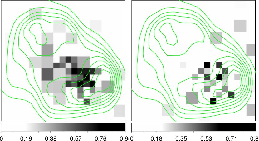
Figure 5: Equivalent width maps of the sulfur line ($\sim 2.43\,{\rm keV}$, left panel) and the argon line ($\sim 3.16\,{\rm keV}$, right panel), both overlaid with the same radio contours as those in Figure 1. The energy range we use to extract the sulfur line emission is 2.33–2.60$\,{\rm keV}$, while the lower- and higher-energy ranges for estimating the continuum emission at the line energy range are 2.27–2.30$\,{\rm keV}$ and 2.63–2.83$\,{\rm keV}$, respectively. For the argon line, the line energy range is 2.87–3.30$\,{\rm keV}$, and the lower- and higher-energy ranges are 2.63–2.83$\,{\rm keV}$ and 3.40–3.90$\,{\rm keV}$, respectively. The color bars are in linear scale in units of $\,{\rm keV}$.

To see where the metal-rich materials’ emission arises, we present the equivalent width (EW) images of S and Ar lines in Figure 5. These images are constructed using a method similar to that used in Jiang & Chen (2010), so as to maximize the statistical quality. Assuming that the line-to-continuum ratio is intrinsically invariable for various detectors, we sum the X-ray counts from XMM-Newton EPIC-MOS and PN and Chandra ACIS observations band-by-band according to componendo. We then rebin the data using an adaptive mesh, with each bin in each narrow band image containing about 10 counts. The intensity of the line emission with the interpolated continuum component subtracted is used as the numerator of the ratio, and the background (estimated from the region surrounding the SNR) is subtracted from the continuum intensity which is used as the denominator. Figure 5 shows that the EW values of both S and Ar lines are only significant in the interior of the southwestern part of the SNR. The caveat here is that the derived continuum images might have lower statistical qualities than the corresponding line emission images and not all the bins can reach 3$\sigma$ significance especially outside the X-ray emission region.

3.2 The Interstellar Environment

3.2.1 Spatial distribution of the ambient clouds

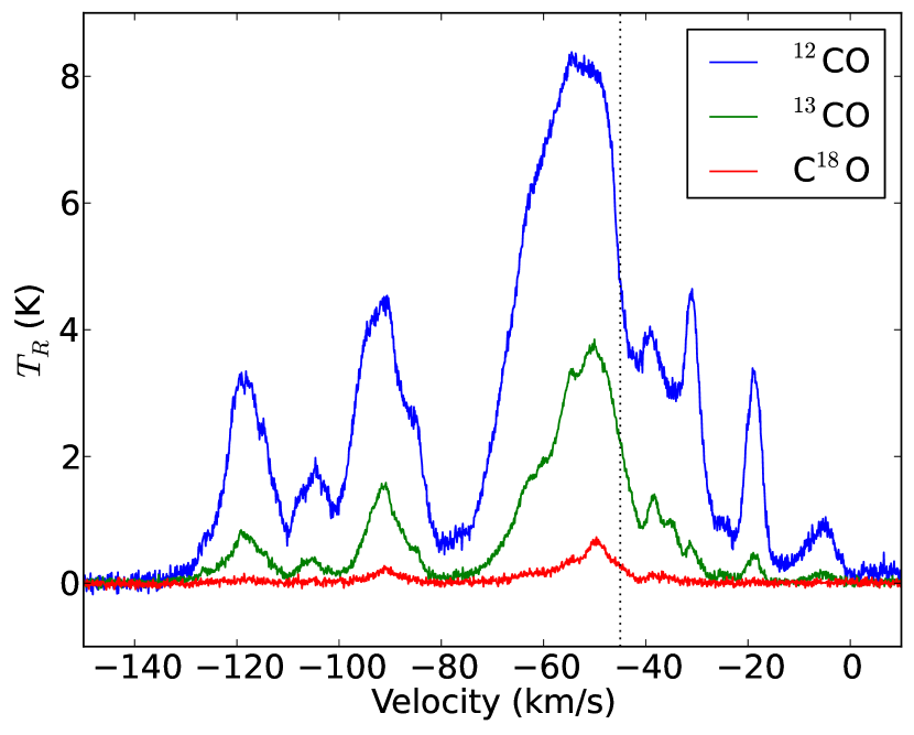
Figure 6: The spectra of ${}^{12}{\rm CO}$ ($J$=1–0), ${}^{13}{\rm CO}$ ($J$=1–0) and ${\rm C}^{18}{\rm O}$ ($J$=1–0) line emission in the FOV. The black dotted vertical line denotes the LSR velocity of the OH maser emission.

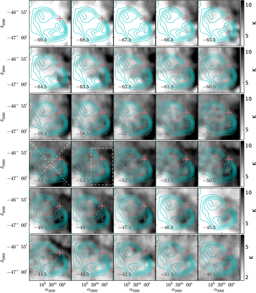
Figure 7: ${}^{12}{\rm CO}$ ($J$=1–0) intensity maps integrated each $1\,{\,{\rm km}\,{\rm s}^{-1}}$ in velocity range $-70$–$-40\,{\,{\rm km}\,{\rm s}^{-1}}$ in linear scale, overlaid with the MOST $843\,{\rm MHz}$ radio continuum contours (at 7 linear scale levels between 0.07 and 0.88$\,{\rm Jy}\,{\rm beam}^{-1}$). The cross indicates the location of the OH (1720$\,{\rm MHz}$) maser spot. The colorbar of the last row of panels is different from those of the other rows due to the relatively low brightness. The dashed lines in the $-54.5\,{\rm km}\,{\rm s}^{-1}$ panel depict the two diagonals of the FOV along which the column density distribution $N({\rm H}_{2})$ of the molecular gas in velocity range $-70$–$-40\,{\,{\rm km}\,{\rm s}^{-1}}$ are measured. The intersection of the diagonals is used as the reference point (see Figure 10). The dashed box in the $-53.5\,{\rm km}\,{\rm s}^{-1}$ panel decipts the region we derive the parameters of the interacting MC.

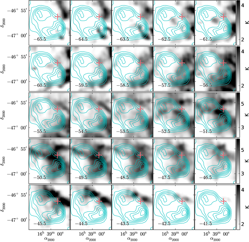
Figure 8: Intensity maps of ${}^{13}{\rm CO}$ ($J$=1–0) observation between $-66\,{\,{\rm km}\,{\rm s}^{-1}}$ and $-41\,{\,{\rm km}\,{\rm s}^{-1}}$ in linear scale. The contours and cross are the same as those in Figure 7. Note the difference in colorbars for different rows.

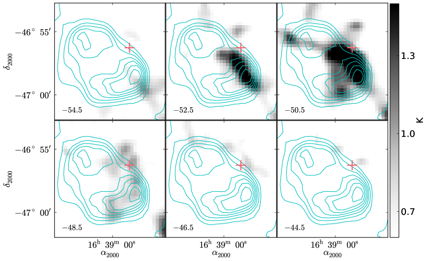
Figure 9: Intensity maps of ${\rm C}^{18}{\rm O}$ ($J$=1–0) observation between $-55\,{\,{\rm km}\,{\rm s}^{-1}}$ and $-45\,{\,{\rm km}\,{\rm s}^{-1}}$ in linear scale. The contours and cross are the same as those in Figure 7.

The average CO spectra over the FOV are shown in Figure 6. There are a number of spectral components along the LOS at the LSR velocities from $V_{\scriptscriptstyle\rm LSR}=-130\,{\,{\rm km}\,{\rm s}^{-1}}$ to $V_{\scriptscriptstyle\rm LSR}=0\,{\,{\rm km}\,{\rm s}^{-1}}$. The LSR velocity of the $1720\,{\rm MHz}$ maser spot, $\sim-45\,{\,{\rm km}\,{\rm s}^{-1}}$, is in the right wing of the line component peaked at $\sim-50\,{\,{\rm km}\,{\rm s}^{-1}}$ which is commonly revealed in the ${}^{12}{\rm CO}$ ($J$=1–0), ${}^{13}{\rm CO}$ ($J$=1–0), and ${\rm C}^{18}{\rm O}$ ($J$=1–0) spectra (see Figure 6). By an examination of the channel maps of the $\sim-50\,{\rm km}\,{\rm s}^{-1}$ line component, we find a morphological correspondence between the western radio boundary of the SNR and a concave surface of MC seen in the ${}^{12}{\rm CO}$ emission at velocity interval $\sim-55$–$-52\,{\,{\rm km}\,{\rm s}^{-1}}$ (see Figure 7). The concaved MC is also remarkable in the integrated ${}^{12}{\rm CO}$ intensity map in interval $-70$–$-40\,{\rm km}\,{\rm s}^{-1}$ within the velocity range of the line profile (see Figure 1). In ${}^{13}{\rm CO}$ emission, a bow-like structure at $\sim-50$–$-48\,{\rm km}\,{\rm s}^{-1}$ seems to match the western radio shell; furthermore, a molecular shell at $\sim-61$–$-58\,{\rm km}\,{\rm s}^{-1}$ perfectly follows the western radio shell of the SNR (see Figure 8). In addition, a section of molecular shell in ${}^{12}{\rm CO}$ emission at $-47.5\,{\rm km}\,{\rm s}^{-1}$ is seen to closely follow the northern radio shell (see Figure 7). Such correspondence is actually only seen in this spectral component by examining the data cubes across the entire LSR velocity span. Around the OH maser position, we can also see some dense molecular gas in the intensity maps (Figure 9) of ${\rm C}^{18}{\rm O}$ emission, which is optically thin and traces molecular cores. The combination of the OH maser and the spatial features of CO emission presented here clearly demonstrates that SNR Kes 41 is in physical contact with the MC at a systemic velocity $V_{\scriptscriptstyle\rm LSR}\sim-50\,{\rm km}\,{\rm s}^{-1}$ in the west and the north, although the broadened CO line profiles of the $\sim-50\,{\rm km}\,{\rm s}^{-1}$ molecular component due to shock disturbance can not be discerned because of line crowding along the LOS.

It is noteworthy that a dense H I cloud at $V_{\scriptscriptstyle\rm LSR}\sim-52\,{\rm km}\,{\rm s}^{-1}$ is situated to the southeast of the SNR (see Figure 1, where the H I intensity image is presented in velocity interval $-55$–$-50\,{\,{\rm km}\,{\rm s}^{-1}}$), and the southeastern radio shell of the SNR seems to follow the surface of the H I cloud. SNR Kes 41 appears to be confined in a cavity enclosed by the molecular cloud in the west and northwest and the H I cloud in the southeast. The archival data show that this H I cloud has an angular size of $\sim 18^{\prime}$.

3.2.2 Parameters of the ambient clouds

We estimate the gas parameters of the $-50\,{\rm km}\,{\rm s}^{-1}$ molecular component in velocity range $-70$–$-40\,{\,{\rm km}\,{\rm s}^{-1}}$ with which the SNR is interacting, and the results are listed in Table 3. The column density and mass of the molecular gas derived may be an upper limit, because there may be irrelevant contributions in the complicated line profiles in ${}^{12}{\rm CO}$ and ${}^{13}{\rm CO}$ emission. For the estimate, we adopt a box region including the main part of the MC in the FOV (see the $-53.5\,{\rm km}\,{\rm s}^{-1}$ panel of Figure 7). Three methods have been utilized to estimate the average molecular column density $N({\rm H}_{2})$, which give a similar value $N({\rm H}_{2})\sim 3$–$5\times 10^{22}\,{\rm cm}^{-2}$. In the first method, we use the mean CO-to-${\rm H}_{2}$ mass conversion factor (known as the X-factor) 1.8$\times 10^{20}\,{\rm cm}^{-2}\,{\rm K}^{-1}\,{\rm km}^{-1}\,{\rm s}$ (Dame et al., 2001) to calculate the molecular column density based on the ${}^{12}{\rm CO}$ ($J$=1–0) emission. In the second method, the ${}^{13}{\rm CO}$ column density is converted to the ${\rm H}_{2}$ column density using $N({\rm H}_{2})/N($${}^{13}{\rm CO}$$)\approx 6.2\times 10^{5}$ (Nagahama et al., 1998), and in the third method, the relation $N({\rm H}_{2})/N($${\rm C}^{18}{\rm O}$$)\approx 7\times 10^{6}$ (Warin et al., 1996) is used for the conversion from ${\rm C}^{18}{\rm O}$ column density to ${\rm H}_{2}$ column density. In the second and the third method, we have assumed a local thermodynamic equilibrium and ${}^{12}{\rm CO}$ ($J$=1–0) line being optically thick, with an excitation temperature of 12.9$\,{\rm K}$ (as obtained from the line peak of ${}^{12}{\rm CO}$ ($J$=1–0)).

Prior to deriving the column densities of ${}^{13}{\rm CO}$ and ${\rm C}^{18}{\rm O}$, we have derived the optical depths $\tau($${}^{13}{\rm CO}$$)\approx 0.6$ and $\tau($${\rm C}^{18}{\rm O}$$)\approx 0.1$, and therefore we treat the ${}^{13}{\rm CO}$ and ${\rm C}^{18}{\rm O}$ emission as optically thin. The $N({\rm H}_{2})$ value obtained from the third method, $\sim 5.1\times 10^{22}\,{\rm cm}^{-2}$, is a little greater than those obtained from the other two methods, and it is probably because ${\rm C}^{18}{\rm O}$ traces denser clouds.

The archival data show that the H I cloud southeast to Kes 41 also has a spectral peak at $-50\,{\rm km}\,{\rm s}^{-1}$ and similar velocity span to the spectral profile of the $-50\,{\rm km}\,{\rm s}^{-1}$ ${}^{12}{\rm CO}$ component. The column density of H I gas ($T_{B}\sim 110\,{\rm K}$) is estimated to be $\sim 5.1\times 10^{21}\,{\rm cm}^{-2}$, using the relation $N$(H I)=1.823$\times 10^{18}T_{B}\Delta v$ on the optically thin assumption (Dickey & Lockman, 1990).

4 Discussion

4.1 SNR environment

Our analysis has revealed that SNR Kes 41 is confined in a cavity enclosed by MCs in the west and the north as well as an H I cloud in the southeast (§ 3.2.1). Some shell-like features of molecular gas also appear to follow the periphery of the SNR. We can give some crude estimates on the gas density of the complicated surrounding environment.

Assuming the LOS size of the $\sim-50\,{\,{\rm km}\,{\rm s}^{-1}}$ MC is similar to its apparent size $\gtrsim 9^{\prime}$ (a lower limit given by the FOV) and using the molecular column density $N({\rm H}_{2})\sim 3$–$5\times 10^{22}\,{\rm cm}^{-2}$, we estimate the molecular density as $n({\rm H}_{2})\lesssim 310$–$510d_{12}^{-1}\,{\rm cm}^{-3}$, where $d_{12}=d/(12\,{\rm kpc})$ is the distance to the MC associated with the SNR in units of the reference value estimated from the maser observation (Koralesky et al., 1998).

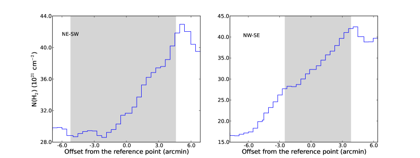
Figure 10: The column density distribution along the dashed lines illustrated in the $-54.5\,{\rm km}\,{\rm s}^{-1}$ panel of Figure 7, the left panel corresponding to the northeast-southwest oriented line and the right panel to the southeast-northwest oriented line. The reference point is the intersection of the lines. The shaded parts indicates the range within the SNR’s radio shell.

Another density estimate can be made from the excavation of the molecular gas in the SNR extent, following the method used in Jiang et al. (2010). We plot the molecular column density distributions of the ${}^{12}{\rm CO}$ line complex in interval $-70$–$-40\,{\,{\rm km}\,{\rm s}^{-1}}$ along the two diagonals of the FOV using X-factor method (see Figure 10). As can be clearly seen, $N({\rm H}_{2})$ generally increases both from the southeast to the northwest and from the northeast to the southwest. Notably, there are peaks/bumps in column density just outside the SNR boundary, which is consistent with the molecular shells described in § 3.2.1. Outside the bumps of the both $N({\rm H}_{2})$ curves, there are platforms at $\sim 4\times 10^{22}\,{\rm cm}^{-2}$; just inside the opposite boundaries, there are lower platforms (wide in the left panel and narrow in the right panel) both at $\sim 2.9\times 10^{22}\,{\rm cm}^{-2}$. The common difference of column density $\sim 1.1\times 10^{22}\,{\rm cm}^{-2}$ can be explained with the removal of molecular gas from the SNR region. Thus the molecular gas originally in the excavated region has a number density $n({\rm H}_{2})\sim 140d_{12}^{-1}\,{\rm cm}^{-3}$ assuming the mean LOS length of the excavated region is similar to the minor axis of the elongated SNR.

If the apparent size of the southeastern H I cloud — that is, $\sim 18^{\prime}$ (see § 3.2.1) — is adopted as the LOS size of the cloud, then the number density of the neutral gas can be estimated from the neutral column density as $n$(H I)$\sim 36d_{12}^{-1}\,{\rm cm}^{-3}$. In the X-ray spectral fitting, a high hydrogen column density of $\sim 5.5$–$8.0\times 10^{22}\,{\rm cm}^{-2}$ is needed to explain the absence of soft ($\lesssim 2.0\,{\rm keV}$) X-ray emission. Apparently, the H I gas towards the Kes 41 direction, which has a column density $\sim 2\times 10^{22}\,{\rm cm}^{-2}$ (Kalberla et al., 2005; Dickey & Lockman, 1990) , is not sufficient to account for the X-ray absorption. However, the $V_{\scriptscriptstyle\rm LSR}\sim-50\,{\rm km}\,{\rm s}^{-1}$ MC, which is associated with the SNR and seems to dominate the CO emission in the direction (Figure 6), has a hydrogen column density $\lesssim 7$–$10\times 10^{22}\,{\rm cm}^{-2}$ and can significantly contribute to the absorbing column. Moreover, the harder X-ray emission in the SW than in the NE (§ 3.1.1) may be consistent with the heavier absorption by the denser molecular gas located in the west.

4.2 SNR physics

4.2.1 Comparisons with main mechanisms and models

(i) Some physical parameters. The density of the X-ray emitting gas interior to the SNR can be estimated using the volume emission measure obtained from the spectral analysis. On the assumption $n_{e}\approx 1.2n_{\scriptscriptstyle\rm H}$ for the densities of electrons and hydrogen atoms, we get $n_{\scriptscriptstyle\rm H}\sim 0.2$–$0.4f^{-1/2}d_{12}^{-1/2}\,{\rm cm}^{-3}$, where $f$ is the filling factor of the hot gas. We estimate the ionization age $t_{i}\sim 4\times 10^{3}$–$1.1\times 10^{5}f^{1/2}d_{12}^{1/2}\,{\rm yr}$ by using the best-fit ionization parameter $n_{e}t$ (also see Table 2).

In the X-ray spectral analysis, the spectral extraction region covers the main part of the X-ray emission. The mass of the hot gas in the region is $\sim 2$–$4f^{3/2}d_{12}^{7/2}M_{\odot}$, which can be regarded as a lower limit. If the hot gas pervades the whole interior of the remnant, we obtain an upper limit of the mass of the hot gas, $\sim 18$–$37f^{1/2}d_{12}^{7/2}M_{\odot}$, assuming a prolate ellipsoid volume ($12.6\times 8.4\times 8.4d_{12}^{3}\,{\rm pc}^{3}$) for the remnant.

(ii) Sedov evolution. Kes 41 has been shown to be surrounded by molecular gas of density $n({\rm H}_{2})\sim 140$–$350\,{\rm cm}^{-3}$ and H I gas of density $n(\mbox{HI})\sim 40\,{\rm cm}^{-3}$. If the SNR follows the Sedov (1959) evolution in the dense ambient gas, and the hot gas temperature obtained from the X-ray spectral fit, $kT_{x}$, is taken to be the emission-measure weighted mean temperature, then the postshock temperature would be $kT_{s}=kT_{x}/1.27$ and the expansion velocity would be $v_{s}=(16kT_{s}/3\bar{\mu}m_{\scriptscriptstyle\rm H})^{1/2}\sim 1.1^{+0.2}_{-0.1}\times 10^{3}\,{\rm km}\,{\rm s}^{-1}$, where the mean atomic weight $\bar{\mu}=0.61$ is used. The dynamic age would be $t=2r/5v_{s}\sim 5.8^{+0.8}_{-1.3}\times 10^{3}d_{12}\,{\rm yr}$ (where $r\sim 13d_{12}\,{\rm pc}$ is the mean radius), and the supernova explosion energy would be $E=(25/4\xi)1.4n_{\scriptscriptstyle 0}m_{\scriptscriptstyle\rm H}r^{3}v_{s}^{2}\sim 2d_{12}^{3}\times 10^{53}\,{\rm erg}$ or $2d_{12}^{3}\times 10^{54}\,{\rm erg}$, for ambient density $n_{\scriptscriptstyle 0}=40\,{\rm cm}^{-3}$ (for H I gas) and $280\,{\rm cm}^{-3}$ (for molecular gas), respectively, where $\xi=2.026$. Such estimates are highly unphysical, because the explosion energy is much higher than the canonical value $10^{51}\,{\rm erg}$. Moreover, the molecules in the surrounding molecular shell (§ 3.2.1) could not survive if the shell were swept up by the SNR shock, given the high shock velocity. Therefore, the assumption of Sedov evolution of Kes 41 in a uniform medium is problematic.

(iii) Evolution in radiative phase. The radiatively cooled rim is one of the scenarios invoked to explain the X-ray thermal composite morphology. If Kes 41 is not considered to be in a pre-existing cavity, then the radiative pressure-driven snowplow (PDS) stage begins at a radius (Cioffi et al., 1988) $r_{\scriptscriptstyle\rm PDS}=2.9E_{51}^{2/7}(n_{\scriptscriptstyle 0}/40\,{\rm cm}^{-3})^{-3/7}\zeta_{m}^{-1/7}\,{\rm pc}$ and an age $t_{\scriptscriptstyle\rm PDS}=3.6\times 10^{3}E_{51}^{3/14}(n_{\scriptscriptstyle 0}/40\,{\rm cm}^{-3})^{-4/7}\zeta_{m}^{-5/14}\,{\rm yr}$, where $E_{51}\equiv E/(10^{51}\,{\rm erg})$ and $\zeta_{m}$ metallicity factor of order unity. If $n_{\scriptscriptstyle 0}=280\,{\rm cm}^{-3}$ for the detected molecular gas, then $r_{\scriptscriptstyle\rm PDS}\sim 1.3\,{\rm pc}$ and $t_{\scriptscriptstyle\rm PDS}\sim 1.8\times 10^{3}\,{\rm yr}$. Compared to the mean radius $\sim 13\,{\rm pc}$ and the ionization age $\gtrsim 4$ kyr, these estimates indicate that the SNR may have entered the radiative phase at an early time. In this scenario, the present velocity of the blast wave is $v_{s}=21[E_{51}(n_{\scriptscriptstyle 0}/40\,{\rm cm}^{-3})^{-36/31}\zeta_{m}^{-5/31}(r/13\,{\rm pc})^{-98/31}]^{31/42}\,{\rm km}\,{\rm s}^{-1}$ (Cioffi et al., 1988; Chen & Slane, 2001), which would be $\sim 4\,{\rm km}\,{\rm s}^{-1}$ for an ambient molecular gas with $n_{\scriptscriptstyle 0}=280\,{\rm cm}^{-3}$, where $E_{51}\sim 1$ and $\zeta_{m}\sim 1$ are assumed for simplicity. With such a shock velocity, the molecular shell can plausibly be explained to be the material swept up by the SNR blast wave. The dynamic age of the remnant is thus given by $t=3.3\times 10^{3}(r/14\,{\rm pc})(v_{s}/413\,{\rm km}\,{\rm s}^{-1})^{-1}[3+n_{\scriptscriptstyle 0}^{-10/31}\zeta_{m}^{-10/31}(r/14\,{\rm pc})^{-10/31}(v_{s}/413\,{\rm km}\,{\rm s}^{-1})^{40/31}]\,{\rm yr}$ (Cioffi et al., 1988; Chen & Slane, 2001), which yields $t\sim 1.8\times 10^{5}\,{\rm yr}$ for a preshock atom gas with $n_{\scriptscriptstyle 0}\sim 40\,{\rm cm}^{-3}$ or $1.0\times 10^{6}\,{\rm yr}$ for a molecular gas with $n_{\scriptscriptstyle 0}\sim 280\,{\rm cm}^{-3}$, respectively, where $r=13\,{\rm pc}$ is adopted. The age estimates here, however, appear to be larger than the ionization age, $t_{i}\sim 4$–$110f^{1/2}d_{12}^{1/2}$ kyr.

(iv) Thermal conduction. Thermal conduction may play a role in shaping the centrally brightened thermal X-ray morphology of Kes 41 by lowering the temperature and increasing the density of the hot gas in the central portion. If the suppression of conduction by magnetic fields can be ignored, the conduction timescale of the hot gas inside the remnant is given by $t_{cond}\sim n_{e}kr^{2}/\kappa$, where the conductivity is given by $\kappa=1.8\times 10^{-5}T_{x}^{5/2}/\ln\Lambda$, with the Coulomb logarithm $\ln\Lambda=29.7+\ln n_{e}^{-1/2}(T_{x}/10^{6}\,{\rm K})$ (Spitzer, 1962). The timescale would thus be $t_{cond}\sim 1.5$–$3.1$ yr, shorter than the ionization age of the X-ray emitting gas.

(v) Cloudlet evaporation. As another popular scenario for thermal composites, cloudlet evaporation is possibly taking place in the remnant interior, since Kes 41 is evolving in an interstellar environment with molecular gas which is usually clumpy and dense clumps can be engulfed by the blast wave. In this case, hot gas with a mass up to $\sim 18$–$37M_{\odot}$ is mostly composed of evaporated gas. This mass is not high enough to substantially dilute the supernova ejecta of a few solar masses, and therefore the evaporation scenario may not be in conflict with the detected metal enrichment. Limited X-ray counts available in the archived observations prevent an estimate of the spatial distribution of such physical parameters as the temperature and density of the hot gas. Even the X-ray surface brightness shows severe asymmetry primarily due to the presence of two brightness peaks (§ 3.1.1), which also makes it difficult to locate the explosion center. All these factors hamper us from presenting a quantitative comparison between the observational properties and the evaporation effect predicted in the White & Long (1991) model.

4.2.2 Metal enrichment

Metal enrichment in the thermal composite SNRs complicate the explanation of the physical mechanism for this class, but meanwhile it is also an important clue to understanding this class of sources. Kes 41 is a thermal composite SNR where the abundances of a few metal species (S and Ar) are elevated. This result motivates its classification as new member of the subclass of “enhanced-abundance” (Lazendic & Slane, 2006) or “ejecta-dominated” (Pannuti et al., 2014a) thermal composite SNRs. This subclass has members amounting to a number of 25–30 (see an updated list of thermal composite SNRs in Table The Metal-Enriched Thermal Composite Supernova Remnant Kesteven 41 (G337.8–0.1) in a Molecular Environment), comprising about 67%–81% of the 36–37 known thermal composites. Sulfur and silicon are the most common enriched species seen among these sources: they are overabundant in 18–19 and 14–15 such SNRs, respectively. The inert elments such as Ar and Ne are overabundant in thirteen thermal composites.

In the case of SNR W44, Shelton et al. (2004a) suggest that central metal enrichment is a factor as important as thermal conduction for the explanation of the centrally-brightened X-ray emission from thermal composite SNRs. They interpret the enhanced metal abundance of W44 as originating from destroyed dust grains within the SNR as well as ejecta enrichment. In Kes 41, the dust destruction scenario may not be favorable because argon, obviously enriched, is an inert element and cannot easily depleted into dust. In the most recent X-ray studies of G352.7$-$0.1 and W51C, metal enrichment is explained to come from supernova ejecta (Pannuti et al., 2014a; Sasaki et al., 2014).

As pointed out by Vink (2012), metal-rich plasma produces more X-ray emission than plasma that is not metal enhanced. In Kes 41, the S and Ar emissions contribute 7% and 2%, respectively, to the broad energy ranges $0.5$–$10\,{\rm keV}$, and the extra abundances of these two metals contribute 3% and 1%, respectively.

4.2.3 Effect of pre-existing cavity

(i) Shock reflection. Thermal composite SNRs are usually associated with dense material (especially MCs), and therefore their progenitor stars are likely to have created a cavity in the dense environment with energetic stellar winds and ionizing radiation. Actually, about ten thermal composites have been found or suggested to evolve in cavities (see Table The Metal-Enriched Thermal Composite Supernova Remnant Kesteven 41 (G337.8–0.1) in a Molecular Environment). When the supernova blast wave hits the cavity wall, a reflected shock can be expected to be sent back inwards and reheat the interior gas including the ejecta to a higher temperature. This is the case suggested for the thermal X-ray composite morphology to SNR Kes 27 (Chen et al., 2008). A similar explanation is also proposed for the thermal composite SNR 3C 397, which is embedded in the edge of a giant MC and confined by a sharp molecular wall (Jiang et al., 2010). The thermal composite SNR W44 appears to be confined in a molecular cavity that is delineated by sharp molecular “edges” in the east, southeast, and southwest, as well as molecular filaments and clumps in other periphery positions (Seta et al., 2004). The metal-enriched X-ray emitting gas in the interior of the SNR may have been reheated by the shock reflected from the cavity wall (which is at least represented by the sharp “edges”).

Kes 41 has been demonstrated here to also be confined in a cavity in a molecular environment. As shown above (§ 4.2.1), both the Sedov and radiative-phase evolution in a uniform dense molecular/H I gas will lead to unreasonable physical parameters, and hence the cavity is not blown by the SNR itself. A collision of the SNR shock with the pre-existing cavity wall thus cannot be ignored. The forward shock of the SNR is drastically decelerated upon the collision. Assuming that the density ratio between the cavity and the wall is much smaller than 1 and adopting the cavity radius $r_{c}\sim 13\,{\rm pc}$, the shock velocity upon the collision can be essentially estimated as (Chen et al., 2003)

$$v_{s}(r_{c})=\left[\frac{E}{2\pi(1.4n_{\scriptscriptstyle 0}m_{\scriptscriptstyle\rm H})r_{c}^{3}}\right]^{1/2},$$ (1)

which is $\lesssim 20E_{51}^{1/2}$ and $50E_{51}^{1/2}\,{\rm km}\,{\rm s}^{-1}$ for $n_{\scriptscriptstyle 0}\gtrsim 280\,{\rm cm}^{-3}$ (for molecular gas) and $n_{\scriptscriptstyle 0}\sim 40\,{\rm cm}^{-3}$ (for H I gas), respectively. Such low velocities indicate that Kes 41 has entered radiative stage right after the blast wave struck the cavity wall. This effect readily explains the lack of X-ray emission in the SNR rim.

The interior gas remains hot and is elevated to a higher temperature by the heating by a reflected shock. This scenario can be tested in combination with the observation result and simplified theory presented by Sgro (1975). For a shock reflection at a dense wall, the temperature ratio between the post–reflected-shock gas and the post–transmitted-shock gas is given by

$$\frac{T_{r}}{T_{t}}=\frac{A}{A_{r}},$$ (2)

where $A_{r}$ is the density contrast between the post–reflected-shock gas and the post–incident-shock gas and $A$ is the wall-to-cavity density contrast, which in turn is a function of $A_{r}$, specifically,

$$A=\frac{3A_{r}(4A_{r}-1)}{\{[3A_{r}(4-A_{r})]^{1/2}-\sqrt{5}(A_{r}-1)\}^{2}}.$$ (3)

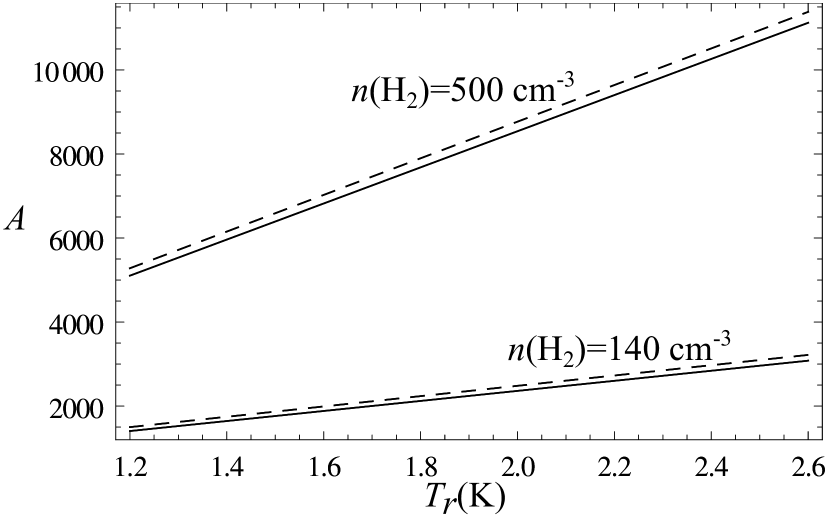
Figure 11: The relation between the wall-to-cavity contrast and the temperature after the heating by the reflected shock. The calculation for two exemplified molecular densities is given. There are two sets of solutions of Equation (3) for each density.

We take $n({\rm H}_{2})\sim 140\,{\rm cm}^{-3}$ as a typical density of the molecular gas and adopt the velocity of the transmitted shock in the molecular cavity wall to be $\sim 20\,{\rm km}\,{\rm s}^{-1}$, which corresponds to $kT_{t}\sim 2.2$ eV. If the observed temperature of the hot gas, $T_{x}$, is adopted for $T_{r}$, we can calculate the dependence of the wall-to-cavity density $A$ on $T_{r}$ in the uncertainty range 1.3–2.6 keV. Figure 11 shows that $A$ is in the range of 1500–3000. Thus a cavity density $\sim 0.1$–$0.2\,{\rm cm}^{-3}$ is implied. If we adopt the observed upper limit $500\,{\rm cm}^{-3}$ for $n({\rm H}_{2})$, almost the same cavity density is inferred. Such a cavity density seems to be of order similar to the observed hot gas density. Here, shock reflection from the dense molecular wall is more efficient than from the H I cloud; actually, the centroids of both the diffuse X-ray emission (§ 3.1.1) and the EW maps of S and Ar (§ 3.1.2) in the southwestern half can be consistent with the reheating primarily by the shock reflected from southwestern dense MC.

(ii) Progenitor’s mass. The pre-existing cavity of Kes 41 should be excavated by the progenitor star, and the progenitor’s mass can be estimated from the cavity size. A linear relation has been found between the progenitor’s mass, $M_{prog}$, and the radius, $R_{b}$, of the bubble blown by the main-sequence wind in a giant MC (Chen et al., 2013):

$$R_{b}\approx(1.22\pm 0.05)(M_{prog}/M_{\odot})-(9.16\pm 1.77)\,{\rm pc}.$$ (4)

If we adopt $R_{b}\approx r_{c}$, the mean radius of the cavity, a stellar mass $18\pm 2M_{\odot}$ is obtained. However, the cavity is not purely confined by molecular gas, but by a giant H I cloud in the southeastern side, and there seems to be a blow-out morphology in the northeast (see Figure 1). Therefore, this mass estimate should be regarded as a lower limit of the progenitor’s mass if the progenitor was not in a binary system, which implies that the progenitor’s spectral type is no later than B0.

(iii) Ejecta in cavities. It can be seen in Table The Metal-Enriched Thermal Composite Supernova Remnant Kesteven 41 (G337.8–0.1) in a Molecular Environment, about half out of the 36-37 known thermal composite SNRs are interacting with adjacent MCs; moreover, eleven or twelve of them are known/thought to be evolving in cavities in dense gas, and most of them exhibit overabundance of metal species. This fact can be explained in the context of the ejecta in pre-existing cavities. An appreciable fraction of supernova ejecta, especially some heavy metal species like Si, are expected to expand at a relatively low velocity (e. g., $\sim 10^{3}\,{\rm km}\,{\rm s}^{-1}$; e. g., Ono et al., 2013, Mao. J. et al. in preparation); for the ejecta expanding in pre-existing cavities, the slow part may have not been substantially mixed or diluted by the interstellar materials by the time when the blast shock is reflected backwards from the cavity wall. They are not only heated by the reverse shock in the early free expansion phase, but also can very possibly be reheated by the reflected shock. Therefore, the hot interior are thus observed to be metal enriched in X-rays.

4.2.4 Recombining effect?

A number of thermal composite SNRs have been revealed to contain recombining plasma (see the rows labeled with “R” in Table The Metal-Enriched Thermal Composite Supernova Remnant Kesteven 41 (G337.8–0.1) in a Molecular Environment). However, the over-ionization in the case of Kes 41 can be neither proven nor disproven by the spectral fitting due to the lack of obvious radiative recombination continuum (RRC) features and H-like lines of the same metal species in the X-ray spectra with insufficient counts. If there is recombining plasma in the remnant, the temperature obtained here using the vnei model may be an overestimate in view of the “apparent” hard continuum raised by the RRC. Deeper X-ray observations are needed to determine if the X-ray-emitting plasma of Kes 41 is indeed overionized.

5 Summary

We have carried out an X-ray observational analysis by revisiting the archival XMM-Newton and Chandra data of the thermal composite SNR Kes 41. We have also conducted and analyzed an observation towards the remnant in ${}^{12}{\rm CO}$, ${}^{13}{\rm CO}$, and ${\rm C}^{18}{\rm O}$ lines. The main results are summarized as follows.

1. Thermal X-ray emission from Kes 41 is detected above 2 keV, which is characterized by distinct S and Ar He-like lines and a brightening in the SNR interior, with a centroid in the emission toward the southwest portion of the SNR.

2. The X-ray emitting gas can be described as an optically thin plasma (at a temperature 1.3–2.6 keV, with an ionization parameter $0.1$–$1.2\times 10^{12}\,{\rm cm}^{-3}\,{\rm s}$) with a NEI model. The metal species S and Ar are found to be over-abundant, with abundances 1.2–2.7 and 1.3–3.8 solar, respectively. They may be enriched by the supernova ejecta.

3. The SNR is found to be associated with a giant MC at a systemic LSR velocity $-50\,{\rm km}\,{\rm s}^{-1}$ and is confined in a cavity delineated by a northern molecular shell, western concave MC with also a discernable shell, and a southeastern H I cloud.

4. The cavity is pre-existing prior to the supernova explosion; it would not be physically realistic to conclude that it was generated by the SNR expansion.

5. Kes 41 seems to have left the adiabatic stage of evolution and entered the radiative phase with an X-ray dim rim just after the SNR shock encountered the dense interstellar medium cavity.

6. Thermal conduction and cloudlet evaporation seem to be feasible mechanisms to interpret the X-ray thermal composite morphology, while the scenario of gas reheating by shock reflected from the cavity wall is quantitatively consistent with the observations.

7. The birth of the SNR in a cavity in a molecular environment implies a mass $\gtrsim 18M_{\odot}$ for the progenitor if it was a single star.

Table 1: Archival Chandra observations for Kes 41 region

			Observation	Exposure	CCD	Good Exposure	Spectral
Obs. ID	R.A.	Decl.	Date	($\,{\rm ksec}$)	chips	($\,{\rm ksec}$)	analysis
12513	${16}^{{\rm h}}{39}^{{\rm m}}{53}\fs 81$	${-46}^{\circ}{57}^{\prime}{45}\farcs 0$	06/27/11	20.4	I0	20.2	yes
12514	${16}^{{\rm h}}{39}^{{\rm m}}{01}\fs 38$	${-46}^{\circ}{49}^{\prime}{45}\farcs 8$	06/10/11	20.0	I1	19.8	no
12516	${16}^{{\rm h}}{39}^{{\rm m}}{06}\fs 95$	${-46}^{\circ}{06}^{\prime}{42}\farcs 5$	06/11/11	19.8	I2	19.5	no
12517	${16}^{{\rm h}}{38}^{{\rm m}}{14}\fs 49$	${-46}^{\circ}{58}^{\prime}{42}\farcs 0$	06/11/11	19.8	I3	19.5	yes
12519	${16}^{{\rm h}}{38}^{{\rm m}}{19}\fs 83$	${-47}^{\circ}{15}^{\prime}{38}\farcs 8$	06/13/11	19.6	S2	19.3	no
12520	${16}^{{\rm h}}{37}^{{\rm m}}{27}\fs 34$	${-47}^{\circ}{07}^{\prime}{37}\farcs 0$	06/13/11	19.6	S3	19.0	yes

Table 2: Spectral fit results with 90% confidence range for the X-ray emitting gas in SNR Kes 41

Parameter	Value
Net count rate ($10^{-3}\,$counts$\,\,{\rm s}$)	$28.05\pm 1.60$
	$7.86\pm 0.49$
	$2.46\pm 0.38$
$N_{\scriptscriptstyle\rm H}$($10^{22}\,{\rm cm}^{-2}$)	6.75${}^{+1.27}_{-1.21}$
$kT_{x}$( keV)	1.80${}^{+0.82}_{-0.47}$
$n_{e}t$($10^{11}\,{\rm s}$ $\,{\rm cm}^{-3}$)	2.06${}^{+9.87}_{-1.56}$
$fn_{e}n_{\scriptscriptstyle\rm H}V/d_{12}^{2}$($10^{57}$cm-3)	1.46${}^{+1.37}_{-0.72}$
[S/H]	1.80${}^{+0.92}_{-0.65}$
[Ar/H]	2.40${}^{+1.42}_{-1.06}$
Reduced $\chi^{2}$ (d.o.f.)	0.99 (54)
Flux ($10^{-12}\,$erg $\,{\rm cm}^{-2}\,{\rm s}^{-1}$)	1.9
$n_{\scriptscriptstyle\rm H}f^{1/2}d_{12}^{1/2}$ ($\,{\rm cm}^{-3}$)	$0.3\pm 0.1$
$t_{i}f^{-1/2}d_{12}^{-1/2}\,(10^{4}\,{\rm yr})$	$1.9^{+8.9}_{-1.5}$

Note. — The abundances of all elements are set to solar abundances except for S and Ar.

Table 3: Derived Parameters of the Ambient Clouds in Velocity Interval $-70$–$-40\,{\,{\rm km}\,{\rm s}^{-1}}$

Lines	$T_{\rm peak}$(K)	$N({\rm H}_{2})\,(10^{22}\,{\rm cm}^{-2})$	$M(10^{4}M_{\odot})\tablenotemark{b}$	$\tau$
${}^{12}{\rm CO}$	9.5	3.8	21.1$d_{12}^{2}$	-
${}^{13}{\rm CO}$	4.5	3.5	19.5$d_{12}^{2}$	0.64
${\rm C}^{18}{\rm O}$	0.95	5.1	28.3$d_{12}^{2}$	0.10
		$N($H I$)\,(10^{21}\,{\rm cm}^{-2})$
H I	110	5.1	1.9$d_{12}^{2}$	-

Table 4: List of Known thermal composite SNRs

	Enriched Metal	Temperature	ionization parameter	MC	Pre-existing	Progenitor’s
SNR Name	Species	$kT_{e}$ (keV)	$n_{e}t$ (s$\,{\rm cm}^{-3}$)	Interaction	Cavity/Shells (Radius/pc)	Mass ($M_{\odot}$)
G0.0+0.0 (Sgr A East)	S, Ar, Ca, Fe, Ni [1,2,3,4]	$kT_{1}\sim$1,		Y, OH	Y ($\sim 5$) [5]	13–20 [1,2,3] ,$\gtrsim 12$
		$kT_{2}\sim$5 [3,2,4]
G6.4–0.1 (W28)	–	$kT_{1}\sim$0.4,	$(n_{e}t)_{1}\sim 1$–$4\times 10^{11}$	Y, OH
		$kT_{2}\sim$0.8 [6,7,8]	[6,7,8]
R:	–	$\sim$0.6 [6,9]	$\sim 9\times 10^{11}$ [6,9]
G21.8–0.6 (Kes 69)	–	$\sim 0.8$ [10,11,12]		Y, OH	Y ($\sim 13$) [13]	$\gtrsim 18$ [14]
G31.9+0.0 (3C 391)	-	$\sim 0.5$–$0.8$ [15,16,8]	$\gtrsim 10^{12}$ [15,8]	Y, OH	Y ($\sim 5$) [18]	$\gtrsim 12$
R:	Mg? [17]	$\sim 0.5$–$0.6$ [17]	$\sim 10^{12}$ [17]
G33.6+0.1 (Kes 79)	S, Ar [19,20]	$kT_{1}\sim 0.2$,		Y?	Y ($\sim 8$) [23,20]	$\gtrsim 14$ [20]
		$kT_{2}\sim 1.1$ [20,21,19,22]	$(n_{e}t)_{2}\sim 3.9\times 10^{10}$
			[20,21,19,22]
G34.7–0.4 (W44)	Ne, Si, S [24]	$kT_{1}\sim 0.3$–0.8,	$\gtrsim 3\times 10^{12}$ [24,8,25]	Y, OH	Y ($\sim 30$) [26]	8–15? [27]
		$kT_{2}\sim 0.9$–4 [24,8,28,25,27]
R:	Mg, Si, S, Ar, Ca [29]	$kT_{1}\sim 0.5$,	$6\times 10^{11}$ [29]
		$kT_{2}\sim 1.0$ [29]
G38.7–1.4	O, Ne [30]	$\sim 0.6$ [30]	$\sim 7\times 10^{12}$ [30]
G41.1–0.3 (3C 397)	O, S, Ca, Fe [31,32,33,34,35]	$kT_{1}\sim 0.21$–$0.25$,	$(n_{e}t)_{1}\sim 3\times 10^{13}$,	Y	Y ($\sim 6$) [36]	$\gtrsim 12$ [14]
		$kT_{2}\sim 1.5$–3.5 [31,35,34]	$(n_{e}t)_{2}\sim 2\times 10^{11}$ [31,35,34]
G43.3–0.2 (W49B)	Si, S, Ar, Ca, Fe, Ni [8,37,38,39,40]	$kT_{1}\sim 0.7$–1.05,		Y?	Y? ($\sim 7$) [23]	$\gtrsim 13$ [23]
		$kT_{2}\sim 1.75$–3.3
		[39,41,42,38,8,40]
R:	Si, S, Ar, Ca, Fe, Ni [43,44,45]	$kT_{1}\sim 0.13$–$0.3$,				$\sim 25$ [37,39,41,40]
		$kT_{2}\sim 1.12$–1.91 [43,44,45]
G49.2–0.7 (W51C)	Ne [46], Mg [46,47], S [48]	0.56–0.74 [46,47,49,48]	0.8–11$\times 10^{11}$	Y, OH		$\gtrsim 20$ [46]
G53.6–2.2 (3C 400.2)	Fe? [50]	$\sim 0.8$ [50]	$\sim 10^{11}$ [50]
G65.3+5.7	–	$\sim 0.25$ [51]
G82.2+5.3 (W63)	Mg, Si, Fe [52]	$kT_{1}\sim 0.2$,
		$kT_{2}\sim 0.6$ [52,53]
G85.4+0.7	O? [54]	1.0 [54]	8$\times 10^{10}$ [54]
G85.9–0.6	O, Fe [54]	1.6 [54]	5$\times 10^{10}$ [54]
G89.0+4.7 (HB21)	Si, S [55,56]	0.62–0.68 [56,55]	$\gtrsim 4\times 10^{11}$ [55,56]	Y
G93.3+6.9 (DA 530)	Si [57]	0.3–0.6 [57,58]	$>4\times 10^{11}$ [57]			$\sim 10$ [57]
G93.7-0.2 (CTB 104A)? [53]	–
G116.9+0.2 (CTB 1)	Mg [55], O, Ne [56]	$kT_{1}\sim 0.2$–0.3,	$\gtrsim 1\times 10^{11}$ [56,55]			$\gtrsim 13$ [56]
		$kT_{2}\sim 3$ [56],
		or $kT_{2}\sim 0.8$ [55]
G132.7+1.3 (HB 3)	Mg [55], or Mg, Ne, O [55]	$\sim 0.3$ [55, 53]		Y?	Y ($\sim 70$) [59]
G156.2+5.7	Si, S [60,61,62]	$kT_{1}\sim 0.45$,	$\sim 1.5\times 10^{11}$ [60,61,62]			$\lesssim 15$ [61]
		$kT_{2}\sim 0.6$ [62,60,63,61]
G160.9+2.6 (HB 9)	–	$\sim 0.8$ [64]		?
G166.0+4.3 (VRO 42.05.01)	S [65]	$\sim 0.7$ [66,67]		?
G189.1+3.0 (IC443)	Mg , S [68,69,65], Si [68,69], Ne [65]	$kT_{1}\sim 0.3$–0.7,	$(n_{e}t)_{1}\gtrsim 10^{12}$ [68,69]	Y, OH	Y ($\sim 11$) [75]	$\gtrsim 15$ [75]
		$kT_{2}\sim 1.0$–1.8
		[68,69,65,70,71,53]
R:	Si, S, Ar [72], Ca, Fe, Ni [73]	$\sim 0.65$ [72,73,74]	$\sim 9.8\times 10^{11}$ [73]
G272.2-3.2	O [76], Ne [77], Si, S, Fe [76,77,78], Ca, Ni [78]	$\sim 0.7$–1.5 [77,76,78,79,80]	2–10$\times 10^{10}$ [77,76,78,80]			(SN Ia) [78,77,76]
G290.1–0.8 (MSH 11–61A)	Si, S [81,82], Mg [81]	$\sim 0.6$–0.9 [82,81]	$>0.1\times 10^{13}$ [82]	?		25–30 [82]
G304.6+0.1 (Kes 17)	Mg? [83,84,85]	$\sim 0.79$–$1.10$ [84,86,85,83]	$\gtrsim 3.7\times 10^{11}$ [84,86,85,83]	Y
G311.5-0.3	–	$\sim 0.98$ [84]		?
G327.4+0.4 (Kes 27)	S, Ca [87], Si [8]	$\sim 0.5$–1.2 [87,53,88,8,89]	$\gtrsim 1\times 10^{11}$ [87,8]		Y [90]
G337.8–0.1 (Kes 41)	S, Ar [91]	$\sim$1.9 [92,91]	$\sim 2\times 10^{11}$ [92,91]	Y, OH	Y ($\sim 13$) [91]	$\gtrsim 18$
G344.7–0.1	Al, Si, S, Ar, Ca, Fe [93,94,95,96]	$\sim$0.8–1.8 [96,95,94,93]	1–4$\times 10^{11}$ [96,95,94,93]	?		(SN Ia) [93]
G346.6-0.2	Ca [97]	$\sim 1.2$ [97,98,84]	$\sim 2.9\times 10^{11}$ [97,84]	Y, OH
R:	–	$\sim$0.3 [99]	$\sim 4.8\times 10^{11}$ [99]
G348.5+0.1 (CTB 37A)	–	0.55–0.83 [84,98,100,101,102]	$>3\times 10^{10}$ [84,102]	Y, OH	? [103]
R:	Si? [102]	$\sim$0.5 [102]	$\sim 1.3\times 10^{12}$ [102]
G352.7–0.1	Si, S [104,105,19], Ar? [19,104]	$0.8$–2.1 [104,105,4]	1–2$\times 10^{10}$ [104,105,19]
G355.6–0.0	Si, S, Ar, Ca [106]	$\sim$0.6 [106,98]
G357.7-0.1 (Tornado)	–	$\sim$0.6 [11,107]		Y,OH
G359.1–0.5	Si, S [108,109]	$kT_{1}\sim 1.1$,		Y, OH	Y ($\sim 28$) [110]
		$kT_{2}\sim 2.0$ [109,111,108,112]
R:	Si, Mg, S [113]	$\sim 0.3$ [113]

Note. — “Y” in the table means “yes”; “?” means that the property is uncertain or controversial; “R” denote that the parameters are derived using the recombining plasma model for the same SNR.

References. — [1] Maeda et al. (2002); [2] Sakano et al. (2004); [3] Park et al. (2005); [4] Koyama et al. (2007); [5] Lee et al. (2008); [6] Zhou et al. (2014); [7] Rho & Borkowski (2002); [8] Kawasaki et al. (2005); [9] Sawada & Koyama (2012); [10] Bocchino et al. (2012); [11] Yusef-Zadeh et al. (2003); [12] Seo & Hui (2013); [13] Zhou et al. (2009); [14] Chen et al. (2013); [15] Chen et al. (2004); [16] Chen & Slane (2001); [17] Ergin et al. (2014); [18] Reach et al. (2002); [19] Giacani et al. (2009); [20] Zhou et al. in preparation; [21] Sun et al. (2004); [22] Auchettl et al. (2014); [23] Chen et al. (2014); [24] Shelton et al. (2004a); [25] Harrus et al. (1997); [26] Seta et al. (2004); [27] Rho et al. (1994); [28] Harrus et al. (2006); [29] Uchida et al. (2012b); [30] Huang et al. (2014); [31] Safi-Harb et al. (2005); [32] Safi-Harb et al. in preparation; [33] Jiang & Chen (2010); [34] Chen et al. (1999); [35] Safi-Harb et al. (2000); [36] Jiang et al. (2010); [37] Keohane et al. (2007); [38] Hwang et al. (2000); [39] Miceli et al. (2006); [40] Lopez et al. (2013b); [41] Lopez et al. (2009); [42] Fujimoto et al. (1995); [43] Lopez et al. (2013a); [44] Ozawa et al. (2009); [45] Miceli et al. (2010); [46] Sasaki et al. (2014); [47] Hanabata et al. (2013); [48] Koo et al. (2005); [49] Koo et al. (2002); [50] Yoshita et al. (2001); [51] Shelton et al. (2004b); [52] Mavromatakis et al. (2004); [53] Rho & Petre (1998); [54] Jackson et al. (2008); [55] Lazendic & Slane (2006); [56] Pannuti et al. (2010); [57] Jiang et al. (2007); [58] Kaplan et al. (2004); [59] Routledge et al. (1991); [60] Yamauchi et al. (1999); [61] Katsuda et al. (2009); [62] Uchida et al. (2012a); [63] Pannuti & Allen (2004); [64] Leahy & Aschenbach (1995); [65] Bocchino et al. (2009); [66] Burrows & Guo (1994); [67] Guo & Burrows (1997); [68] Troja et al. (2006); [69] Troja et al. (2008); [70] Petre et al. (1988); [71] Keohane et al. (1997); [72] Yamaguchi et al. (2009); [73] Ohnishi et al. (2014); [74] Kawasaki et al. (2002); [75] Su et al. (2014); [76] Sánchez-Ayaso et al. (2013); [77] McEntaffer et al. (2013); [78] Sezer & Gök (2012); [79] Greiner et al. (1994); [80] Harrus et al. (2001); [81] Slane et al. (2002); [82] García et al. (2012); [83] Gelfand et al. (2013); [84] Pannuti et al. (2014b); [85] Gök & Sezer (2012); [86] Combi et al. (2010b); [87] Chen et al. (2008); [88] Enoguchi et al. (2002); [89] Seward et al. (1996); [90] McClure-Griffiths et al. (2001); [91] this paper; [92] Combi et al. (2008); [93] Yamaguchi et al. (2012); [94] Giacani et al. (2011); [95] Yamauchi et al. (2005); [96] Combi et al. (2010a); [97] Sezer et al. (2011b); [98] Yamauchi et al. (2008); [99] Yamauchi et al. (2013); [100] Aharonian et al. (2008); [101] Sezer et al. (2011a); [102] Yamauchi et al. (2014); [103] Maxted et al. (2013); [104] Pannuti et al. (2014a); [105] Kinugasa et al. (1998); [106] Minami et al. (2013); [107] Gaensler et al. (2003); [108] Bamba et al. (2000); [109] Bamba et al. (2009); [110] Uchida et al. (1992); [111] Egger & Sun (1998); [112] Sakano et al. (2002); [113] Ohnishi et al. (2011);

References

- Aharonian et al. (2008) Aharonian, F., et al. 2008, A&A, 490, 685
- Anders & Grevesse (1989) Anders, E., & Grevesse, N. 1989, Geochim. Cosmochim. Acta, 53, 197
- Auchettl et al. (2014) Auchettl, K., Slane, P., & Castro, D. 2014, ApJ, 783, 32
- Bamba et al. (2009) Bamba, A., Yamazaki, R., Kohri, K., Matsumoto, H., Wagner, S., Pühlhofer, G., & Kosack, K. 2009, ApJ, 691, 1854
- Bamba et al. (2000) Bamba, A., Yokogawa, J., Sakano, M., & Koyama, K. 2000, PASJ, 52, 259
- Bocchino et al. (2009) Bocchino, F., Miceli, M., & Troja, E. 2009, A&A, 498, 139
- Bocchino et al. (2012) Bocchino, F., et al. 2012, A&A, 541, A152
- Burrows & Guo (1994) Burrows, D. N., & Guo, Z. 1994, ApJ, 421, L19
- Casandjian & Grenier (2008) Casandjian, J.-M., & Grenier, I. A. 2008, A&A, 489, 849
- Caswell (2004) Caswell, J. L. 2004, MNRAS, 349, 99
- Caswell et al. (1975) Caswell, J. L., Murray, J. D., Roger, R. S., Cole, D. J., & Cooke, D. J. 1975, A&A, 45, 239
- Chen et al. (2014) Chen, Y., Jiang, B., Zhou, P., Su, Y., Zhou, X., Li, H., & Zhang, X. 2014, in IAU Symposium, Vol. 296, Supernova Environmental Impacts, ed. A. Ray & R. A. McCray, 170–177
- Chen et al. (2008) Chen, Y., Seward, F. D., Sun, M., & Li, J.-t. 2008, ApJ, 676, 1040
- Chen & Slane (2001) Chen, Y., & Slane, P. O. 2001, ApJ, 563, 202
- Chen et al. (2004) Chen, Y., Su, Y., Slane, P. O., & Wang, Q. D. 2004, ApJ, 616, 885
- Chen et al. (1999) Chen, Y., Sun, M., Wang, Z.-R., & Yin, Q. F. 1999, ApJ, 520, 737
- Chen et al. (2003) Chen, Y., Zhang, F., Williams, R. M., & Wang, Q. D. 2003, ApJ, 595, 227
- Chen et al. (2013) Chen, Y., Zhou, P., & Chu, Y.-H. 2013, ApJ, 769, L16
- Cioffi et al. (1988) Cioffi, D. F., McKee, C. F., & Bertschinger, E. 1988, ApJ, 334, 252
- Combi et al. (2008) Combi, J. A., Albacete-Colombo, J. F., & Martí, J. 2008, A&A, 488, L25
- Combi et al. (2010a) Combi, J. A., et al. 2010a, A&A, 522, A50
- Combi et al. (2010b) —. 2010b, A&A, 523, A76
- Dame et al. (2001) Dame, T. M., Hartmann, D., & Thaddeus, P. 2001, ApJ, 547, 792
- Dickey & Lockman (1990) Dickey, J. M., & Lockman, F. J. 1990, ARA&A, 28, 215
- Egger & Sun (1998) Egger, R., & Sun, X. 1998, in Lecture Notes in Physics, Berlin Springer Verlag, Vol. 506, IAU Colloq. 166: The Local Bubble and Beyond, ed. D. Breitschwerdt, M. J. Freyberg, & J. Truemper, 417–420
- Enoguchi et al. (2002) Enoguchi, H., Tsunemi, H., Miyata, E., & Yoshita, K. 2002, PASJ, 54, 229
- Ergin & Ercan (2012) Ergin, T., & Ercan, E. N. 2012, in American Institute of Physics Conference Series, Vol. 1505, American Institute of Physics Conference Series, ed. F. A. Aharonian, W. Hofmann, & F. M. Rieger, 265–268
- Ergin et al. (2014) Ergin, T., Sezer, A., Saha, L., Majumdar, P., Chatterjee, A., Bayirli, A., & Ercan, E. N. 2014, ApJ, 790, 65
- Frail & Mitchell (1998) Frail, D. A., & Mitchell, G. F. 1998, ApJ, 508, 690
- Fujimoto et al. (1995) Fujimoto, R., et al. 1995, PASJ, 47, L31
- Gaensler et al. (2003) Gaensler, B. M., Fogel, J. K. J., Slane, P. O., Miller, J. M., Wijnands, R., Eikenberry, S. S., & Lewin, W. H. G. 2003, ApJ, 594, L35
- García et al. (2012) García, F., Combi, J. A., Albacete-Colombo, J. F., Romero, G. E., Bocchino, F., & López-Santiago, J. 2012, A&A, 546, A91
- Gelfand et al. (2013) Gelfand, J. D., Castro, D., Slane, P. O., Temim, T., Hughes, J. P., & Rakowski, C. 2013, ApJ, 777, 148
- Giacani et al. (2011) Giacani, E., Smith, M. J. S., Dubner, G., & Loiseau, N. 2011, A&A, 531, A138
- Giacani et al. (2009) Giacani, E., Smith, M. J. S., Dubner, G., Loiseau, N., Castelletti, G., & Paron, S. 2009, A&A, 507, 841
- Gök & Sezer (2012) Gök, F., & Sezer, A. 2012, MNRAS, 423, 1215
- Green et al. (1997) Green, A. J., Frail, D. A., Goss, W. M., & Otrupcek, R. 1997, AJ, 114, 2058
- Greiner et al. (1994) Greiner, J., Egger, R., & Aschenbach, B. 1994, A&A, 286, L35
- Guo & Burrows (1997) Guo, Z., & Burrows, D. N. 1997, ApJ, 480, L51
- Hanabata et al. (2013) Hanabata, Y., Sawada, M., Katagiri, H., Bamba, A., & Fukazawa, Y. 2013, PASJ, 65, 42
- Harrus et al. (2006) Harrus, I., Smith, R., Slane, P., & Hughes, J. 2006, in ESA Special Publication, Vol. 604, The X-ray Universe 2005, ed. A. Wilson, 369
- Harrus et al. (1997) Harrus, I. M., Hughes, J. P., Singh, K. P., Koyama, K., & Asaoka, I. 1997, ApJ, 488, 781
- Harrus et al. (2001) Harrus, I. M., Slane, P. O., Smith, R. K., & Hughes, J. P. 2001, ApJ, 552, 614
- Huang et al. (2014) Huang, R. H. H., Wu, J. H. K., Hui, C. Y., Seo, K. A., Trepl, L., & Kong, A. K. H. 2014, ApJ, 785, 118
- Hwang et al. (2000) Hwang, U., Petre, R., & Hughes, J. P. 2000, ApJ, 532, 970
- Jackson et al. (2008) Jackson, M. S., Safi-Harb, S., Kothes, R., & Foster, T. 2008, ApJ, 674, 936
- Jiang & Chen (2010) Jiang, B., & Chen, Y. 2010, ScChG, 53, 267
- Jiang et al. (2010) Jiang, B., Chen, Y., Wang, J., Su, Y., Zhou, X., Safi-Harb, S., & DeLaney, T. 2010, ApJ, 712, 1147
- Jiang et al. (2007) Jiang, B., Chen, Y., & Wang, Q. D. 2007, ApJ, 670, 1142
- Jones et al. (1998) Jones, T. W., et al. 1998, PASP, 110, 125
- Kalberla et al. (2005) Kalberla, P. M. W., Burton, W. B., Hartmann, D., Arnal, E. M., Bajaja, E., Morras, R., & Pöppel, W. G. L. 2005, A&A, 440, 775
- Kaplan et al. (2004) Kaplan, D. L., Frail, D. A., Gaensler, B. M., Gotthelf, E. V., Kulkarni, S. R., Slane, P. O., & Nechita, A. 2004, ApJS, 153, 269
- Katsuda et al. (2009) Katsuda, S., Petre, R., Hwang, U., Yamaguchi, H., Mori, K., & Tsunemi, H. 2009, PASJ, 61, 155
- Kawasaki et al. (2005) Kawasaki, M., Ozaki, M., Nagase, F., Inoue, H., & Petre, R. 2005, ApJ, 631, 935
- Kawasaki et al. (2002) Kawasaki, M. T., Ozaki, M., Nagase, F., Masai, K., Ishida, M., & Petre, R. 2002, ApJ, 572, 897
- Keohane et al. (1997) Keohane, J. W., Petre, R., Gotthelf, E. V., Ozaki, M., & Koyama, K. 1997, ApJ, 484, 350
- Keohane et al. (2007) Keohane, J. W., Reach, W. T., Rho, J., & Jarrett, T. H. 2007, ApJ, 654, 938
- Kinugasa et al. (1998) Kinugasa, K., Torii, K., Tsunemi, H., Yamauchi, S., Koyama, K., & Dotani, T. 1998, PASJ, 50, 249
- Koo et al. (2002) Koo, B.-C., Lee, J.-J., & Seward, F. D. 2002, AJ, 123, 1629
- Koo et al. (2005) Koo, B.-C., Lee, J.-J., Seward, F. D., & Moon, D.-S. 2005, ApJ, 633, 946
- Koralesky et al. (1998) Koralesky, B., Frail, D. A., Goss, W. M., Claussen, M. J., & Green, A. J. 1998, AJ, 116, 1323
- Koyama et al. (2007) Koyama, K., Uchiyama, H., Hyodo, Y., Matsumoto, H., Tsuru, T. G., Ozaki, M., Maeda, Y., & Murakami, H. 2007, PASJ, 59, 237
- Ladd et al. (2005) Ladd, N., Purcell, C., Wong, T., & Robertson, S. 2005, PASA, 22, 62
- Lazendic & Slane (2006) Lazendic, J. S., & Slane, P. O. 2006, ApJ, 647, 350
- Leahy & Aschenbach (1995) Leahy, D. A., & Aschenbach, B. 1995, A&A, 293, 853
- Lee et al. (2008) Lee, S., et al. 2008, ApJ, 674, 247
- Lockett et al. (1999) Lockett, P., Gauthier, E., & Elitzur, M. 1999, ApJ, 511, 235
- Lopez et al. (2013a) Lopez, L. A., Pearson, S., Ramirez-Ruiz, E., Castro, D., Yamaguchi, H., Slane, P. O., & Smith, R. K. 2013a, ApJ, 777, 145
- Lopez et al. (2013b) Lopez, L. A., Ramirez-Ruiz, E., Castro, D., & Pearson, S. 2013b, ApJ, 764, 50
- Lopez et al. (2009) Lopez, L. A., Ramirez-Ruiz, E., Pooley, D. A., & Jeltema, T. E. 2009, ApJ, 691, 875
- Maeda et al. (2002) Maeda, Y., et al. 2002, ApJ, 570, 671
- Mavromatakis et al. (2004) Mavromatakis, F., Aschenbach, B., Boumis, P., & Papamastorakis, J. 2004, A&A, 415, 1051
- Maxted et al. (2013) Maxted, N. I., et al. 2013, MNRAS, 434, 2188
- McClure-Griffiths et al. (2005) McClure-Griffiths, N. M., Dickey, J. M., Gaensler, B. M., Green, A. J., Haverkorn, M., & Strasser, S. 2005, ApJS, 158, 178
- McClure-Griffiths et al. (2001) McClure-Griffiths, N. M., Green, A. J., Dickey, J. M., Gaensler, B. M., Haynes, R. F., & Wieringa, M. H. 2001, ApJ, 551, 394
- McEntaffer et al. (2013) McEntaffer, R. L., Grieves, N., DeRoo, C., & Brantseg, T. 2013, ApJ, 774, 120
- Miceli et al. (2010) Miceli, M., Bocchino, F., Decourchelle, A., Ballet, J., & Reale, F. 2010, A&A, 514, L2
- Miceli et al. (2006) Miceli, M., Decourchelle, A., Ballet, J., Bocchino, F., Hughes, J. P., Hwang, U., & Petre, R. 2006, A&A, 453, 567
- Minami et al. (2013) Minami, S., Ota, N., Yamauchi, S., & Koyama, K. 2013, PASJ, 65, 99
- Nagahama et al. (1998) Nagahama, T., Mizuno, A., Ogawa, H., & Fukui, Y. 1998, AJ, 116, 336
- Ohnishi et al. (2011) Ohnishi, T., Koyama, K., Tsuru, T. G., Masai, K., Yamaguchi, H., & Ozawa, M. 2011, PASJ, 63, 527
- Ohnishi et al. (2014) Ohnishi, T., Uchida, H., Tsuru, T. G., Koyama, K., Masai, K., & Sawada, M. 2014, ApJ, 784, 74
- Ono et al. (2013) Ono, M., Nagataki, S., Ito, H., Lee, S.-H., Mao, J., Hashimoto, M.-a., & Tolstov, A. 2013, ApJ, 773, 161
- Ozawa et al. (2009) Ozawa, M., Koyama, K., Yamaguchi, H., Masai, K., & Tamagawa, T. 2009, ApJ, 706, L71
- Pannuti & Allen (2004) Pannuti, T. G., & Allen, G. E. 2004, Advances in Space Research, 33, 434
- Pannuti et al. (2014a) Pannuti, T. G., Kargaltsev, O., Napier, J. P., & Brehm, D. 2014a, ApJ, 782, 102
- Pannuti et al. (2010) Pannuti, T. G., Rho, J., Borkowski, K. J., & Cameron, P. B. 2010, AJ, 140, 1787
- Pannuti et al. (2014b) Pannuti, T. G., Rho, J., Heinke, C. O., & Moffitt, W. P. 2014b, AJ, 147, 55
- Park et al. (2005) Park, S., et al. 2005, ApJ, 631, 964
- Petre et al. (1988) Petre, R., Szymkowiak, A. E., Seward, F. D., & Willingale, R. 1988, ApJ, 335, 215
- Reach et al. (2002) Reach, W. T., Rho, J., Jarrett, T. H., & Lagage, P.-O. 2002, ApJ, 564, 302
- Rho & Borkowski (2002) Rho, J., & Borkowski, K. J. 2002, ApJ, 575, 201
- Rho & Petre (1998) Rho, J., & Petre, R. 1998, ApJ, 503, L167
- Rho et al. (1994) Rho, J., Petre, R., Schlegel, E. M., & Hester, J. J. 1994, ApJ, 430, 757
- Routledge et al. (1991) Routledge, D., Dewdney, P. E., Landecker, T. L., & Vaneldik, J. F. 1991, A&A, 247, 529
- Safi-Harb et al. (2005) Safi-Harb, S., Dubner, G., Petre, R., Holt, S. S., & Durouchoux, P. 2005, ApJ, 618, 321
- Safi-Harb et al. (2000) Safi-Harb, S., Petre, R., Arnaud, K. A., Keohane, J. W., Borkowski, K. J., Dyer, K. K., Reynolds, S. P., & Hughes, J. P. 2000, ApJ, 545, 922
- Sakano et al. (2002) Sakano, M., Koyama, K., Murakami, H., Maeda, Y., & Yamauchi, S. 2002, ApJS, 138, 19
- Sakano et al. (2004) Sakano, M., Warwick, R. S., Decourchelle, A., & Predehl, P. 2004, MNRAS, 350, 129
- Sánchez-Ayaso et al. (2013) Sánchez-Ayaso, E., Combi, J. A., Bocchino, F., Albacete-Colombo, J. F., López-Santiago, J., Martí, J., & Castro, E. 2013, A&A, 552, A52
- Sasaki et al. (2014) Sasaki, M., Heinitz, C., Warth, G., & Pühlhofer, G. 2014, A&A, 563, A9
- Sawada & Koyama (2012) Sawada, M., & Koyama, K. 2012, PASJ, 64, 81
- Sedov (1959) Sedov, L. I. 1959, Similarity and Dimensional Methods in Mechanics
- Seo & Hui (2013) Seo, K.-A., & Hui, C. Y. 2013, Journal of Astronomy and Space Sciences, 30, 87
- Seta et al. (2004) Seta, M., Hasegawa, T., Sakamoto, S., Oka, T., Sawada, T., Inutsuka, S.-i., Koyama, H., & Hayashi, M. 2004, AJ, 127, 1098
- Seward et al. (1996) Seward, F. D., Kearns, K. E., & Rhode, K. L. 1996, ApJ, 471, 887
- Sezer & Gök (2012) Sezer, A., & Gök, F. 2012, MNRAS, 421, 3538
- Sezer et al. (2011a) Sezer, A., Gök, F., Hudaverdi, M., & Ercan, E. N. 2011a, MNRAS, 417, 1387
- Sezer et al. (2011b) Sezer, A., Gök, F., Hudaverdi, M., Kimura, M., & Ercan, E. N. 2011b, MNRAS, 415, 301
- Sgro (1975) Sgro, A. G. 1975, ApJ, 197, 621
- Shaver & Goss (1970) Shaver, P. A., & Goss, W. M. 1970, Australian Journal of Physics Astrophysical Supplement, 14, 133
- Shelton et al. (2004a) Shelton, R. L., Kuntz, K. D., & Petre, R. 2004a, ApJ, 611, 906
- Shelton et al. (2004b) —. 2004b, ApJ, 615, 275
- Slane et al. (2002) Slane, P., Smith, R. K., Hughes, J. P., & Petre, R. 2002, ApJ, 564, 284
- Spitzer (1962) Spitzer, L. 1962, Physics of Fully Ionized Gases
- Su et al. (2014) Su, Y., Fang, M., Yang, J., Zhou, P., & Chen, Y. 2014, ArXiv e-prints
- Sun et al. (2004) Sun, M., Seward, F. D., Smith, R. K., & Slane, P. O. 2004, ApJ, 605, 742
- Troja et al. (2008) Troja, E., Bocchino, F., Miceli, M., & Reale, F. 2008, A&A, 485, 777
- Troja et al. (2006) Troja, E., Bocchino, F., & Reale, F. 2006, ApJ, 649, 258
- Uchida et al. (2012a) Uchida, H., Tsunemi, H., Katsuda, S., Mori, K., Petre, R., & Yamaguchi, H. 2012a, PASJ, 64, 61
- Uchida et al. (2012b) Uchida, H., et al. 2012b, PASJ, 64, 141
- Uchida et al. (1992) Uchida, K. I., Morris, M., Bally, J., Pound, M., & Yusef-Zadeh, F. 1992, ApJ, 398, 128
- Vink (2012) Vink, J. 2012, A&A Rev., 20, 49
- Wardle & Yusef-Zadeh (2002) Wardle, M., & Yusef-Zadeh, F. 2002, Science, 296, 2350
- Warin et al. (1996) Warin, S., Castets, A., Langer, W. D., Wilson, R. W., & Pagani, L. 1996, A&A, 306, 935
- White & Long (1991) White, R. L., & Long, K. S. 1991, ApJ, 373, 543
- Whiteoak & Green (1996) Whiteoak, J. B. Z., & Green, A. J. 1996, A&AS, 118, 329
- Wilner et al. (1998) Wilner, D. J., Reynolds, S. P., & Moffett, D. A. 1998, AJ, 115, 247
- Yamaguchi et al. (2009) Yamaguchi, H., Ozawa, M., Koyama, K., Masai, K., Hiraga, J. S., Ozaki, M., & Yonetoku, D. 2009, ApJ, 705, L6
- Yamaguchi et al. (2012) Yamaguchi, H., Tanaka, M., Maeda, K., Slane, P. O., Foster, A., Smith, R. K., Katsuda, S., & Yoshii, R. 2012, ApJ, 749, 137
- Yamauchi et al. (1999) Yamauchi, S., Koyama, K., Tomida, H., Yokogawa, J., & Tamura, K. 1999, PASJ, 51, 13
- Yamauchi et al. (2014) Yamauchi, S., Minami, S., Ota, N., & Koyama, K. 2014, PASJ, 66, 2
- Yamauchi et al. (2013) Yamauchi, S., Nobukawa, M., Koyama, K., & Yonemori, M. 2013, PASJ, 65, 6
- Yamauchi et al. (2005) Yamauchi, S., Ueno, M., Koyama, K., & Bamba, A. 2005, PASJ, 57, 459
- Yamauchi et al. (2008) —. 2008, PASJ, 60, 1143
- Yoshita et al. (2001) Yoshita, K., Tsunemi, H., Miyata, E., & Mori, K. 2001, PASJ, 53, 93
- Yusef-Zadeh et al. (2003) Yusef-Zadeh, F., Wardle, M., Rho, J., & Sakano, M. 2003, ApJ, 585, 319
- Zhou et al. (2014) Zhou, P., Safi-Harb, S., Chen, Y., Zhang, X., Jiang, B., & Ferrand, G. 2014, ApJ, 791, 87
- Zhou et al. (2009) Zhou, X., Chen, Y., Su, Y., & Yang, J. 2009, ApJ, 691, 516