Lick-index entanglement and biased diagnostic of stellar populations in galaxies

Abstract

The Lick-index spectrophotometric system is investigated in its inherent statistical and operational properties to ease a more appropriate use for astrophysical studies. Non-Gaussian effects in the index standardization procedure suggest that a minimum S/N ratio has to be reached by spectral data, such as $S/N\ga 5$ px^-1 for a spectral resolution $R\sim 2000$. In addition, index (re-)definition in terms of narrow-band “color” should be preferred over the classical pseudo-equivalent width scheme.

The overlapping wavelength range among different indices is also an issue, as it may lead the latter ones to correlate, beyond any strictly physical relationship. The nested configuration of the Fe5335, Fe5270 indices, and the so-called “Mg complex” (including Mg₁, Mg₂ and Mgb) is analysed, in this context, by assessing the implied bias when joining entangled features into “global” diagnostic meta-indices, like the perused [MgFe] metallicity tracer. The perturbing effect of [OIII]₅₀₀₇ and [NI]₅₁₉₉ forbidden gas emission on Fe5015 and Mgb absorption features is considered, and an updated correction scheme is proposed when using [OIII]₅₀₀₇ as a proxy to appraise H$\beta$ residual emission. When applied to present-day elliptical galaxy population, the revised H$\beta$ scale leads, on average, to 20-30% younger age estimates.

Finally, the misleading role of the christening element in Lick-based chemical analyses is illustrated for the striking case of Fe4531. In fact, while Iron is nominally the main contributor to the observed feature in high-resolution spectra, we have shown that the Fe4531 index actually maximizes its responsiveness to Titanium abundance.

1 Introduction

Since its very beginning, the Lick-index system was intentionally conceived as a tool to characterize elliptical galaxies and other old stellar systems (Faber, Burstein, & Dressler, 1977; Faber et al., 1985; Davies et al., 1987; Gorgas, Efstathiou, & Aragon Salamanca, 1990). Only a few relevant absorption lines were originally taken into account, at the sides of the strong Magnesium feature around 5175 Å, which blends the molecular hydride MgH and the atomic doublet Mgb (Mould, 1978). Together with the 4000 Å break, the Mg “valley” has since long been recognized as the most outstanding pattern in the optical spectrum of galaxies (Öhman, 1934; Wood, 1963; Spinrad & Wood, 1965).

The immediate interest for galaxy investigation directly drove a parallel effort to extend the index database also to cool stars (e.g. Burstein et al., 1984) for their evident link with the study of old galaxies through population synthesis applications. At the same time, this also led to a more definite settlement of the whole index system, greatly extended by new additions from the Lick Image Dissector Scanner (IDS) data archive including all the relevant absorption features in the optical wavelength range comprised between the 4000 Å break and the Balmer $H\alpha$ line (Gorgas et al., 1993; Worthey et al., 1994). The original emphasis to old stellar populations extended then to hot and warm stars (Worthey & Ottaviani, 1997) to account for ongoing star formation scenarios, as in late-type galaxies (e.g. Mollá, Hardy, & Beauchamp, 1999; Walcher et al., 2006; Pérez, Sánchez-Blázquez, & Zurita, 2009).

In more recent years, other spectroscopic methods have been complementing the original Lick approach, aimed at tackling galaxy properties at a finer or coarser detail level. High-resolution spectroscopy (say at the typical resolving power, $R\ga 2000$ or so, of current extragalactic surveys) certainly added valuable clues, on this line. On the opposite side, a panchromatic analysis relying on low-resolution fitting of galaxy SED (often assembled by straight flux conversion of integrated broad-band magnitudes) also became an increasingly popular way to deal with massive wealth of galaxy data, in order to characterize redshift distribution and other outstanding evolutionary features on a statistical basis (see Walcher et al., 2011; Conroy, 2013, for excellent reviews on these subjects).

For several reasons, however, none of these techniques is free from some limitations. From its side, high-resolution spectroscopy may be constrained by the intervening role of galaxy dynamics; at a typical velocity dispersion of $\sigma_{v}\simeq 300$ km s^-1, the induced line broadening limits the effective resolving power at $R\la 1000$. On the other hand, global fitting of galaxy SED carries on all the inherent uncertainty in absolute flux calibration of the observations, especially when matching data from different observing sources and over distant wavelength ranges. In addition, to quote Walcher et al. (2011), we have to remind that, as “the uncertainties are dominated by the uncertainties in the SED modeling itself, thus one has to be very cautious about the interpretations when selecting samples where a specific type of model is preferred.”

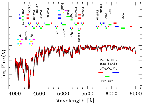
Figure 1: A global view of the Lick-index wavelength distribution. The original set of 21 indices (Worthey et al., 1994) has been complemented by the four Worthey & Ottaviani (1997) new Balmer indices (namely, H$\delta$ and H$\gamma$, in their “wide” and “narrow” version) and the González (1993) [OIII] index, as labelled in the plot. The index map is superposed to a synthetic stellar spectrum with $[T_{\rm eff},\log g,Z]=[4750~{}{\rm K},2.00,Z_{\odot}]$ from the Bluered theoretical library (Bertone et al., 2004, 2008), degraded to match the Lick spectral resolution of 8.5 Å FWHM.

For all these reasons, narrow-band spectrophotometry still remains, in most cases, the elective (and often the only viable) tool to assess in finer detail the evolutionary status of galaxies and other unresolved stellar aggregates both in local and high-redshift environments (see Bernardi et al., 2006; Carson & Nichol, 2010; Dobos et al., 2012, for recent contributions). Such a broad range of applications urges, however, a more careful in-depth analysis of the inherent properties of the Lick system in order to enable its appropriate use in the investigation of single stars and integrated stellar systems. This motivated the present work.

When dealing with Lick indices, two intervening difficulties may in principle affect our conclusions. A first, and often underrated issue (discussed here in Sec. 2) deals with the index standardization, that is with the process to make index measurements, from different sources or observing circumstances, to consistently compare eachother. Quite importantly, this process should not be confused with the calibration procedure, as the first requires ab initio that index definition could lead anytime to a “fair” statistical realization of a normal statistical variable according to the Central Limit Theorem (see, e.g. Sachs, 1984, for a more rigorous theoretical settlement of the problem.) While a satisfactory attention is devoted in the relevant literature to suitably calibrate observing data (Worthey et al., 1994; Trager et al., 1998; Cardiel et al., 1998), this cannot assure, by itself, that a “standard” settlement of the derived index estimates is always achieved.

The latter feature we have to remind is that indices may not be completely independent each one and, how we will show in Sec. 3, some degree of redundancy occurs in many cases. For instance, sometimes two indices may share the same pseudo-continuum window, or two feature windows are partly or fully superposed etc.. Even more sneaky, some redundancy may also appear when, under certain conditions, the same chemical element that constrains the main feature also affect the surrounding pseudo-continuum, thus masking or vanishing the index sensitivity to its abundance. When changing temperature or other fundamental parameters of stars, a “hidden” chemical element may abruptly appear at some point with its lines, and superpose to the other absorption features affecting the corresponding indices. This is, for instance, the classical case of the onset of TiO molecular bands in cool stars perturbing, among others, the Mg₂ and Fe5270 indices (Buzzoni, Gariboldi, & Mantegazza, 1992; Tantalo & Chiosi, 2004; Buzzoni, Bertone, & Chavez, 2009a).

A further range of problems deal with more physical environment conditions of stellar populations. Most importantly, a natural effect of fresh star formation on the integrated spectrum of galaxies is line emission driven by the residual interstellar gas. Along the Lick-index range, this results in enhanced Hydrogen Balmer lines and, depending on the overall thermodynamical conditions, also in [OIII] forbidden emission at 4363, 4959 and 5007 Å (see Kennicutt, 1992, for excellent explanatory examples). On the other hand, Oxygen and $H\beta$ emission is triggered even at the vanishing star formation rates observed in most elliptical galaxies (Caldwell, 1984; Phillips et al., 1986; Bettoni & Buson, 1987; Volkov, 1990; Sarzi et al., 2010; Crocker et al., 2011) due, at the very least, to the contribution of the planetary nebulae (see Kehrig et al., 2012, for an example), and this could easily bias our conclusions if we use $H\beta$ (absorption) strength to constrain galaxy age.

In this paper we will carry on our analysis from two independent points of view, starting from the expected behaviour according to index properties and checking theoretical predictions by means of a tuned set of spectroscopic observations for a sample of twenty elliptical galaxies. Our relevant conclusions, and a reasoned summary of the the manifold variables at work is proposed in Sec. 4 of the paper.

2 Index technicalities

Up to the 70’s, low-resolution sampling of galaxy and stellar energy distribution was mainly pursued by narrow-band photometry. Popular multicolor systems included, for instance, those of Strömgren (1956), the DDO system of McClure & van den Bergh (1968), the multicolor set of Spinrad & Taylor (1969) or the 10-color system of Faber (1973). In this framework, the Lick system stands out for its innovative approach to the problem, tackled now from a purely spectroscopic point of view.

Indeed, such a new “spectroscopic mood” is inherent in the Lick-index definition. The procedure applies in fact to low-resolution ($R\sim 500$) spectra and aims at deriving the strength of a number of absorption features through a measure of their pseudo-equivalent width. Indices are therefore measured in Å, maintaining the magnitude scale only for those few cases of molecular bands (Worthey et al., 1994). The original set of 21 indices was defined by Worthey et al. (1994) and slightly adapted to more suitably fit with extragalactic targets by Trager et al. (1998). A complement to include the full Balmer line series in the optical wavelength range led Worthey & Ottaviani (1997) to add four new indices, that match $H\gamma$ and $H\delta$ lines with “narrow” and “wide” windows. With these additions, the full Lick system consists of 25 indices. Apart, it is worth including in our analysis also an extemporary addition to the standard set due to González (1993), in order to account for [OIII] emission in the spectrum of star-forming galaxies. Note that this is the only index aimed at measuring an emission feature (see Fig. 1).

According to Worthey’s (1994) original precepts, the key quantity of any Lick index is the ratio

$${\cal R}=\overline{\big{(}{f\over f_{c}}\big{)}}={1\over w}\ \int_{w}\left({f\over f_{c}}\right)_{\lambda}d\lambda.$$ (1)

$\cal R$ is therefore an average, along the $w$-wide feature window, of the apparent flux density, $f(\lambda)$, normalized to the (pseudo)-continuum level, $f_{c}(\lambda)$, linearly interpolated at the same wavelength. Two adjacent bands, on both side of the feature, provide the baseline for the interpolated process. With these prescriptions, the index then directly follows either as

$$I({\rm\AA})=w\ \big{(}1-{\cal R}\big{)}$$ (2)

or

$$I({\rm mag})=-2.5\ \log{\cal R}$$ (3)

depending whether we want to express it in Å, as pseudo-equivalent width, or in magnitude scale. Clearly, both definitions are fully equivalent and easily reversible as

$$I({\rm\AA})=w\ \big{[}1-10^{-0.4\ {\rm I(mag)}}\big{]}$$ (4)

or

$$I({\rm mag})=-2.5\ \log\big{[}1-{{\rm I(\AA)}\over w}\big{]},$$ (5)

and the use of Å or magnitudes is just a matter of “flavor”, as we have been mentioning above (see, for instance, Brodie & Huchra 1990, Colless et al. 1999, or Sánchez-Blázquez et al. 2006a for alternative non-standard notations). As a rule, both eq. (2) and (3) are positive for absorption features and negative for emission ones.

2.1 Standardization constraints

In spite of its established popularity and extensive use in a broad range of stellar and extra-galactic studies, a well recognized drawback of the Lick system is its ambigous standardization procedure. A meticulous analysis in this sense has been attempted by Trager et al. (1998) to account for the macroscopic limits of the IDS database due to the somewhat fickle technical performance of the instrument. Some inconstancy in the spectrum wavelength scale is, for instance, a recognized issue, and even the spectral resolution (about 8.5 Å FWHM, see Worthey & Ottaviani, 1997) cannot be firmly established due to slightly unpredictable behaviour of the instrument output with time (Worthey et al., 1994). In addition, and quite importantly, one has to notice that the whole IDS data set is in fact not flux-calibrated (Worthey et al., 1994), thus taking over the instrument (slightly variable) response curve. For all this, any comparison between external data sources in the literature must forcedly rely, as a minimum, on the observation of a common grid of standard stars (e.g. Worthey et al., 1994; Gorgas et al., 1993; Buzzoni, Gariboldi, & Mantegazza, 1992; Buzzoni, Mantegazza, & Gariboldi, 1994; Buzzoni et al., 2001, among others).

A few attempts have been made, in the recent literature, to refine the index estimates from the operational point of view to secure on more solid bases the observed output. The work of Rogers et al. (2010) is certainly the most relevant one, in this sense, as it especially focus on the problem of a fair settlment of the pseudo-continuum level (through the so-called “boosted median continuum” method) to derive a more confident feature strength, also overcoming those recognized cases of unphysical output (for example with nominally “emission” indices tracing, in fact, absoption features etc.).

As a matter of fact, any more or less elaborated empirical matching procedure, however, cannot overcome a more subtle but inherent difficulty in the standardization process of the Lick system. In fact, the way one leads to compute $\cal R$ according to eq. (1) is a direct “heritage” of high-resolution spectroscopy, where the measure is always carried out on preliminarily continuum-rectified spectra. However, this is clearly not the case for the (unfluxed) Lick spectra, where possibly steep continuum gradients are in principle an issue. According to statistics theory, the consequence is that ratio $\cal R$ may display strongly non-Gaussian properties (see Marsiglia, 1964, and especially Fig. 1 therein for an eloquent example) making the analysis of its distribution a hard (and in some cases hopeless) task. In other words, this implies that, in general, any effort to reproduce the system may not obey the Central Limit Theorem so that its convergence is not assured a priori (Marsiglia, 1965).

In this framework, it is therefore of central interest to explore the real contraints that make $\cal R$ behave normally. For this, let us briefly consider the more general problem of the stochastic behaviour of a statistical variable $r$ being the ratio of two normal variables $x$ and $y$, namely $r=y/x$. It has been firmly demonstrated (Geary, 1930; Hinkley, 1969; Hayya, Armstrong, & Gressis, 1975) that $r$ tends to behave like $y$ if the range of variation of $x$ (that is $dx/\overline{x}$), approaches zero and the $x$ variable is “unlikely to assume negative values” (Geary, 1930). If this is the case, then $x$ tends to behave as a (positive) “constant” and $xr$ would resemble the $y$ distribution (Hayya, Armstrong, & Gressis, 1975). Under these assumptions, the $r^{\prime}=\overline{y}/\overline{x}$ ratio will display a normal distribution and its average $\overline{r^{\prime}}$ tends to be an unbiased proxy of $\overline{r}$. In our terms, therefore, the crucial constraints that ensure both index Gaussianity and its fair reproducibility directly deals with two issues: from one hand we need a “small” range of variation for $df_{c}/\overline{f_{c}}$; on the other hand, we need to assess the condition for which $\overline{r^{\prime}}\to\overline{r}$.

To further proceed with our analysis, let us preliminarily assume the relative variation of $f_{c}$ to be “small”, indeed, so that we are allowed to set up a linear expansion for $f_{c}$ around $\lambda_{o}$, the central wavelength within the feature window of width $w$:

$${1\over f_{c}}=\big{[}\ {1\over\overline{f_{c}}}-{1\over\overline{f_{c}}^{2}}\ {\partial f_{c}\over\partial\lambda}\ (\lambda-\lambda_{o})\big{]}={1\over\overline{f_{c}}}\ \big{[}1-{{\alpha(\lambda-\lambda_{o})}\over\overline{f_{c}}}\big{]}.$$ (6)

In previous equation, $\alpha=\partial f_{c}/\partial\lambda$ and, by definition, $({\alpha w})=df_{c}$ is the maximum excursion of $f_{c}(\lambda)$ within the feature window.

By implementing eq. (6) into eq. (1) we have

$${\cal R}={1\over\overline{f_{c}}}\big{[}{{\int_{w}f(\lambda)d\lambda}\over w}-{\alpha\over{w\overline{f_{c}}}}\int_{w}f(\lambda)(\lambda-\lambda_{o})d\lambda\big{]}.$$ (7)

If we now multiply and divide by $w\int f(\lambda)d\lambda$ the last term of the equation, with little arithmetic we can re-arrange the equation and write

$${\cal R}={\cal R^{\prime}}\big{[}1-{{\alpha w}\over\overline{f_{c}}}{{\langle\delta\lambda\rangle}\over w}\big{]}={\cal R^{\prime}}\big{[}1-{{\langle\delta\lambda\rangle}\over w}\left({{df_{c}}\over\overline{f_{c}}}\right)^{\rm max}\big{]}$$ (8)

being

$${\cal R^{\prime}}=\big{(}{\overline{f}\over\overline{f_{c}}}\big{)},$$ (9)

and $\langle\delta\lambda\rangle/w$ the relative displacement, within the feature window, of the line centroid with respect to $\lambda_{o}$, in consequence of symmetry departure due to the spectral slope. According to eq. (8), therefore, ${\cal R^{\prime}}$ tends to become a fair proxy of ${\cal R}$ if

$$\Big{|}1-{{\cal R}\over{\cal R^{\prime}}}\Big{|}\la\left({{\langle\delta\lambda\rangle}\over w}\right)\left({{df_{c}}\over\overline{f_{c}}}\right)^{\rm max}.$$ (10)

The maximim relative excursion $(df_{c}/\overline{f_{c}})^{\rm max}$ is, evidently, the key figure in this process as it directly constrains both r.h. factors in eq. (10). It may be wise to assess the allowed range of this parameter in terms of the stochastic fluctuation range of $f_{c}$ within the same window, the latter being directly related to the signal-to-noise ratio ($S/N$) of our data, so that we can set

$$\big{(}{df_{c}\over\overline{f_{c}}}\big{)}^{\rm max}\la\ k\big{[}{\sigma(f_{c})\over\overline{f_{c}}}\big{]}={k\over S/N},$$ (11)

with $k$ a tuning factor. We will show, in the next section, that a minimum signal-to-noise ratio of $S/N\sim 20$ is required for ${\cal R^{\prime}}$ to behave normally (Hayya, Armstrong, & Gressis, 1975). With this figure, if we choose to tentatively accept a pseudocontinuum excursion within a $\pm 3\sigma$ range of the random noise, then $k\la 6$ and $(df_{c}/\overline{f_{c}})^{\rm max}\la 0.3$, so that one could actually verify numerically that

$$\Big{|}1-{{\cal R}\over{\cal R^{\prime}}}\Big{|}\la 0.01.$$ (12)

With the previous assumptions, this means that, within a 1% accuracy, the ratio ${\cal R^{\prime}}$ eventually becomes an unbiased estimator of ${\cal R}$, thus assuring ${\cal R}$ to behave normally, too. Our first conclusion is therefore that Geary’s (1930) prescriptions require pseudo-continumm not to exceed a $\pm 30$% relative variation within the feature window for any Lick index to obey the Central Limit Theorem, and display a Gaussian distribution.

2.2 Random-error estimate

A range of more or less entangled attempts have been proposed across the literature to derive a general and self-consistent estimate of the statistical uncertainty to be related to narrow-band indices (Rich, 1988; Brodie & Huchra, 1990; Carollo, Danziger, & Buson, 1993; González, 1993; Cardiel et al., 1998; Trager et al., 1998). Yet, this effort does not seem to have led to any firm and straightforward pathway to assess the index random-error estimate. Quite different formal approaches can be found among authors depending whether the intervening noise sources (including photon statistics, flat-fielding procedure, sky subtraction etc.) are considered individually or to a somewhat aggregated level in the analysis. In addition, as we have been discussing in previous section, with the Lick system one has to deal with the duality of index definition, sometimes seen in terms of pseudo-colors and sometimes in terms of pseudo-equivalent widths.

In its general form, by simple differentiation of eq. (2) and (3), the expected internal uncertainty of a Lick index expressed in magnitude is

$$\sigma(I)_{\rm mag}=1.08\big{[}{\sigma({\cal R})\over{\cal R}}\big{]}.$$ (13)

On the contrary, if we chose to express the index in pseudo-equivalent width, then

$$\sigma(I)_{\rm{\AA}}=\big{[}{\sigma({\cal R})\over{\cal R}}\big{]}(w-I_{\rm{\AA}})$$ (14)

In both cases, the crucial quantity that we have to assess is the $\sigma({\cal R})/{\cal R}$ ratio. A useful contribution to settle the problem has come from Vollmann & Eversberg (2006), dealing with the error estimate in equivalent-width measurements from high-resolution spectroscopy. Under many aspects, their results directly apply to our framework providing the caveats of previous section to be properly accounted for in our analysis and to observe at “sufficient S/N within the continuum” (Vollmann & Eversberg, 2006). If the ${\cal R}^{\prime}$ ratio could be an effective proxy of ${\cal R}$, then the variance of ${\cal R}$ directly derives from error propagation as

$$\sigma^{2}({\cal R})=\big{[}{\partial{\cal R}\over\partial f}\sigma(f)\big{]}^{2}+\big{[}{\partial{\cal R}\over\partial f_{c}}\sigma(f_{c})\big{]}^{2},$$ (15)

which implies

$$\sigma^{2}({\cal R})=\big{(}{1\over f^{2}_{c}}\sigma^{2}_{f}\big{)}+\big{(}{f^{2}\over f^{4}_{c}}\sigma^{2}_{fc}\big{)}={f^{2}\over f^{2}_{c}}\ {\sigma^{2}_{f}\over f^{2}}+{f^{2}\over f^{2}_{c}}\ {\sigma^{2}_{fc}\over f^{2}_{c}}.$$ (16)

In case a similar S/N ratio along the relevant range of our spectrum can be assumed, so that $({\sigma(f)/f})\sim({\sigma(fc)/f_{c}})$, a final compact form can be achieved for previous equations such as

$${\sigma({\cal R})\over{\cal R}}\simeq{\sigma({\cal R})\over{\cal R}^{\prime}}={\sqrt{2}\over(S/N)_{idx}}.$$ (17)

Quite importantly, note that the value of $S/N$ in eq. (17) refers to the integrated figure along the feature and continuum windows. Providing to observe a spectrum with an original $(S/N)_{obs}$ ratio per pixel and a dispersion $\theta$ Å px^-1, the resulting $(S/N)_{idx}$ by sampling flux along a window $w$ Å wide is, of course,

$$(S/N)_{idx}=(S/N)_{obs}\sqrt{{w\over\theta}}$$ (18)

Table 1: Harmonic average^(a) (${\cal W}$), feature (w) and continuum (W) window width for the extended set of Lick indices

Index	${\cal W}$	w	W	Index	${\cal W}$	w	W
	[Å]				[Å]
H$\delta_{W}$	50.1	38.8	70.6	$[{\rm OIII}]$	32.7	20.0	90.0
H$\delta_{N}$	30.5	21.3	53.8	Fe5015	54.6	76.3	42.5
CN1	48.2	35.0	77.5	Mg1	86.1	65.0	127.5
CN2	42.0	35.0	52.5	Mg2	63.8	42.5	127.5
Ca4227	15.0	12.5	18.8	Mgb	33.1	32.5	33.7
G4300	33.7	35.0	32.5	Fe5270	43.4	40.0	47.5
H$\gamma_{W}$	58.6	43.8	88.8	Fe5335	27.8	40.0	21.2
H$\gamma_{N}$	31.9	21.0	66.3	Fe5406	24.0	27.5	21.3
Fe4383	32.5	51.3	23.8	Fe5709	29.1	23.8	37.5
Ca4455	23.1	22.5	23.7	Fe5782	21.7	20.0	23.7
Fe4531	35.1	45.0	28.8	NaD	36.3	32.5	41.0
Fe4668	47.3	86.3	32.5	TiO1	72.3	57.5	97.5
H$\beta$	31.6	28.8	35.0	TiO2	97.0	82.5	117.5
(a) According to eq. (21).

In their work, (Hayya, Armstrong, & Gressis, 1975) set the limit of general validity of this formal approach through a detailed Monte Carlo analysis. Converting their results to our specific framework (see, in particular, their Fig. 1), we conclude that eq. (17) is a robust estimator of the relative standard deviation of ${\cal R}$ providing to work with $(S/N)_{idx}>20$.

On the basis of our discussion we can eventually re-arrange previous eq. (13) and (14) in their final form, respectively:

$$\sigma(I)_{\rm mag}={\sqrt{2\theta\over{\cal W}}}\ \ {1.09~{}~{}~{}~{}\over(S/N)_{obs}},$$ (19)

and

$$\sigma(I)_{\rm\AA}={\sqrt{2\theta\over{\cal W}}}\ \ {w\over(S/N)_{obs}}\ \big{(}1-{I_{\rm\AA}\over w}\big{)}.$$ (20)

For “shallow” lines (that is those with $[I({\rm\AA})/w]\ll 1$), we can simply neglect the last factor in previous equation, thus leading to an even more compact (though slightly overestimated) form for the standard deviation.

In both eq. (19) and (20), ${\cal W}$ is the harmonic average of the feature ($w$) and continuum ($W$) window widths:

$${2\over{\cal W}}=\big{(}{1\over w}+{1\over W}\big{)}.$$ (21)

For reader’s better convenience, the value of $\cal W$, together with the feature and the full (i.e. red+blue) continuum windows for the extended set of Lick indices is summarized in Table 1.

Taking eq. (19) and (20) as a reference, in Fig. 2 we compare the observed standard deviation of primary Lick stellar calibrators, according to Worthey et al. (1994, see, in particular, Table 1 therein) and Worthey & Ottaviani (1997) with our expected error distribution for a spectrum of $(S/N)_{\rm obs}=30$.

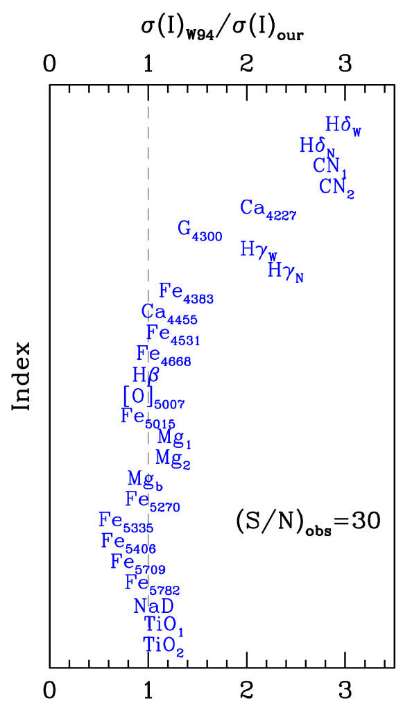
Figure 2: The expected index standard deviation $\sigma(I)_{our}$, according to eq. (20), for an assumed spectral $S/N\sim 30$ is compared with the empirical estimate from the Lick primary calibrators, as from Table 1 of Worthey (1994) and Worthey & Ottaviani (1997). The uncertainty for [OIII]₅₀₀₇ has been estimated from the González (1993) data, as from Table 4.1 therein, by scaling down his figures to $S/N=30$. Notice that Lick IDS spectra lack any stable intensity response, a feature that prevents any firm assessment of the S/N ratio of the original data (Faber & Jackson, 1976; Worthey et al., 1994). A remarkably good agreement is found, however, with our theoretical predictions, as far as “red” indices (about $\lambda\ga 4350$ Å) are concerned. A notable worsening in the Lick calibration accuracy is evident at shorter wavelength, likely due to poorer detector performance and statistical drawbacks inherent to index definition, as discussed in the text.

Although no firm appraisal can be done of original IDS data in terms of S/N ratio, a problem extensively discussed by Worthey et al. (1994), nonetheless there is point to believe that the S/N assumed in the present derivation is similar to the floor imposed on the IDS spectra by small-scale flat-fielding problems. In this framework one could recognize our statistical analysis as an instructive excercise to put in a more standard context the inherent uncertainty of Worthey’s et al reference dataset, at least as far as indices “redder” than $\sim 4350$ Å are concerned.

Note, however, a dramatic worsening of the IDS performance in the blue, where index accuracy quickly degrades. This trend can now easily be understood on the basis of our previous statistical arguments. At shorter wavelength, in fact, the combined effects of a worse IDS response and an intrinsic drop of SED for stars of intermediate and late spectral type all conspire in the sense of exacerbating any spectral slope, thus departing from the standard Gaussian scenario (in force of eq. 10), and adding further extra-volatility to Lick-index calculation.

3 Index entanglement and redundancy

A closer look to Fig. 1 data shows that about 25% of the covered wavelength range actually contributes to the definition of two or more indices leading, on average, to a  $1.5$ oversampling fraction. Such a redundancy evidently calls for a more detailed analysis of the possible bias effects that in some cases make indices inter-dependent in their stochastic fluctuation, that is beyond any strictly physical relationship.

This is certainly the case of some intervening emission, that superposes to absorption features ($H\beta$ is a typical example in this sense), but also partly or fully overlapping pseudo-continuum windows, in common with different indices, may induce some degree of correlation in the corresponding output (as for the blue sidebands of Ca4455 or Fe5335, fully comprised within the Fe4383 and Fe5270 red sidebands, respectively). This may also happen to feature windows, as shown for instance by Mgb, fully comprised within the Mg₂ central band. Finally, a further possibility is that the entire feature contributes to the pseudo-continuum window of another index: the case of Fe5335, is explanatory in this regard being fully nested into the red sideband of Mg₂ and Mg₁.

In this section we want therefore to assess some illustrative cases giving, when possible, a guideline for a more general application of our results. The theoretical predictions that come from the reference discussion of Sec. 2, will be accompanied by an empirical check, that could allow us a clean assessment of the different situations sketched above.

3.1 Radial spectroscopy of elliptical galaxies as a robust empirical check

For our aims it is convenient to rely on a set of spectroscopic data for a sample of 20 early-type (mainly elliticals) galaxies observed with the 2.12m telescope of the “G. Haro” Observatory of Cananea (Mexico) in a series of runs along years 1996/97. These observations are part of a more general exhaustive study on spectroscopic gradients across the surface of galaxies and its physical implications for galaxy evolution (Carrasco et al., 1995; Buzzoni et al., 2009b, 2015). It is clearly beyond the scope of this work to dig further into the original scientific issue and the detailed data reduction analysis (the reader could be addressed to the cited references for a full review). We just want to recall here the basic information to characterize the sample in view of its possible relevance as an independent tool to probe our theoretical output.

The spectra have been collected with a long-slit Böller & Chivens Cassegrain spectrograph equipped with a 300 gr/mm grating, that provided a dispersion of 67 Å/mm along a 4200-6000 Å  wavelength interval. Spectral resolution was set to 5 Å (FWHM) throughout ($R=\lambda/\Delta\lambda\sim 1000$) Galaxy targets were typically exposed along one hour ($3\times 1200^{\prime\prime}$ frames) centering along galaxy major axis. The resulting spectra have been wavelength- and flux-calibrated according to standard procedures, and have then been rebinned in the spatial domain such as to sample galaxy radius at 3-5 values of distance symmetrically placed with respect to the center, roughly up to one effective radius (see Buzzoni et al., 2009b, for an example). The rebinning procedure allowed us to greatly improve the $S/N$ ratio especially in the outermost regions such as to work there with $S/N\ga 25$ px^-1, a figure that quickly improved to $S/N\ga 80$ px^-1 toward the center.

The relevant information of the galaxy sample is summarized in Table 2. From the RC3 catalog (de Vaucouleurs et al., 1991) we report morphological classification, absolute $B$-band magnitude (M_B), and apparent $(B-V)$ color within one effective radius ($r_{e}$). In addition, in the last two columns we added, respectively, the radial fraction sampled with our spectra (r/r_e) (see Buzzoni et al., 2009b, for further details), and a flag for galaxies with reported emission. In this regard, one asterisk mark a confirmed [OII]₃₇₂₇ emission, as in the Bettoni & Buson (1987) catalog, while with a double asterisk we marked targets with evident [OIII]₅₀₀₇ and/or H$\beta$ central emission in our spectra.

Table 2: The galaxy database

NGC	Type	MB	(B-V)	$r_{max}/r_{e}$	emission?
1587	E1p	-21.19	1.04	0.2	* *
1588	Ep	-19.91	1.00	0.5
2685	S0-a	-19.09	0.94	0.8	*
2764	S0	-19.55	0.71	1.2	* *
3245	S0	-20.09	0.89	1.0
3489	S0-a	-19.23	0.85	0.8	* *
3607	E-S0	-20.00	0.93	0.4	*
4111	S0-a	-19.16	0.88	3.0	*
4125	E6p	-21.27	0.94	0.4	*
4278	E1	-19.35	0.96	1.0	* *
4374	E1	-21.05	1.00	0.6	*
4382	S0-a	-20.50	0.89	0.3
4472	E2	-21.71	0.98	0.8
4649	E2	-21.47	1.00	0.5
4742	E4	-19.35	0.79	1.3	*
5576	E3	-20.14	0.90	0.4
5812	E0	-20.44	1.04	0.4
5866	S0-a	-20.00	0.93	0.7	* *
5982	E3	-21.38	0.94	0.7	*
6166	E2p	-22.96	1.03	0.4	*

For the galaxies of Table 2, Buzzoni et al. (2009b, 2015) have derived the complete set of 17 standard Lick indices (including the [OIII]₅₀₀₇ feature), from G4300 to Fe5709. These data provide us with a useful reference to perform, for each index, a series of statistically equivalent realizations. This can be carried out in force of the supposed central symmetry of the galaxy spectral properties. Even in case of spectroscopic radial gradients, in fact, a similar stellar population has to be hosted at the same distance on opposite sides of the galaxy leading to a nominally identical set of absorption indices. Clearly, any systematic deviation from this pure folding effect may be worth of attention in our analysis.

Note that, as we deal with index differences, our method is quite insensitive to standardization problems (zero points settlement, calibration drifts etc.), although we obviously magnify the internal random errors of our analysis by a factor of $\sqrt{2}$. About 80 couples of index differences have been computed across the full galaxy sample, for a total of roughly 1400 measures for the full set of 17 indices.

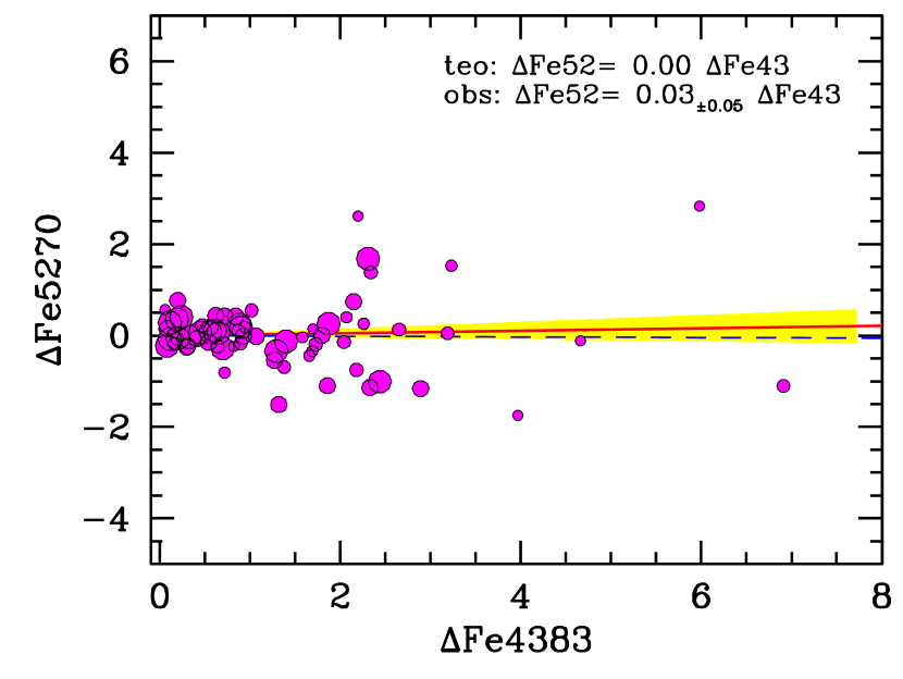
Figure 3: The envisaged $\Delta$-$\Delta$ test among galaxy spectroscopic indices in the (Buzzoni et al., 2009b, 2015) galaxy sample (see text for details) is explained here for the illustrative case of Fe4383 (index “x”) and Fe5270 (index “y”). If we assume the source of “left – right” index difference to be only of stochastic nature, then no correlation has to be expected between $\Delta$ Fe4383 and $\Delta$ Fe5270. A least-square linear fit to the data, in the form of $\Delta y=\alpha\Delta x$, actually provides $\alpha=0.03_{\pm 0.05}$ (solid line with the yellow fan marking the $\pm 1\sigma$ standard deviation of the slope estimator), fully consistent with a flat trend (dashed line), as expected for this case. Just as a guideline, notice that the dot size in the plot is smaller for index measurements at farther radial distances from galaxy center.

Just as an explanatory example, to illustrate our approach, we show in Fig. 3 the $\Delta$-$\Delta$ index distribution for two FeI indices, namely Fe5270 versus Fe4383. Each point in the plot comes from the following procedure. For two slices at the same radial distance (on opposite side) of a given galaxy, we computed $\delta x$ as the “left – right” difference of the Fe4383 index measurements. The same is done for Fe5270, deriving $\delta y$. We then set $\Delta x=|\delta x|$ and obtain the sign of $\delta x$ as ${\rm sign}_{x}=\delta(x)/\Delta(x)$, so that $\Delta y={\rm sign}_{x}\delta y$. Though, from a physical point of view, both indices should correlate with Iron abundance, no mutual influence can exist for their relative variation. As a consequence, their “left-right” differences must be statistically independent over the entire galaxy sample. This is actually confirmed by the least-square fit to the data in the figure (68 points in total), which provides $\alpha=0.03_{\pm 0.05}$.

3.2 Ménage à trois: H$\beta$, [OIII]₅₀₀₇ and Fe5015

The wavelength region of galaxy spectra around 5000 Å may be heavily prone to the effects of gas emission. In particular, the $H\beta$ and Fe5015 strengths could be affected, the first resulting from the parallel action of stellar absorption and gas emission, the latter because of the possible [OIII] 5007Å appearence (see Fig. 4). This issue is of central relevance as, within the Lick system, the $H\beta$ index is the most suitable one to place strong constraints to the age of unresolved stellar aggregates (e.g. Buzzoni, Mantegazza, & Gariboldi, 1994; Bressan, Chiosi, & Tantalo, 1996; Vazdekis et al., 1996; Tantalo, Chiosi, & Bressan, 1998; Kobayashi & Arimoto, 1999; Maraston & Thomas, 2000; Trager et al., 2000; Thomas et al., 2005; Fusi Pecci et al., 2005; Sánchez-Blázquez et al., 2006b; Peletier et al., 2007, and many others) due to its close response to the temperature location of the Main Sequence Turn Off stars (Gorgas et al., 1993; Buzzoni, 1995; Buzzoni, Bertone, & Chavez, 2009a).

A proper correction of this effect is not quite a straightforward task, especially when modest amounts of emission do not appear as “surging” features in the spectra and rather hide making absorption line-depth artificially shallower. If uncorrected, this effect would bias age estimates toward older values. A first attempt to account for $H\beta_{e}$ residual emission is due to González (1993), who assumed the [OIII]₅₀₀₇ index to be a confident proxy for $H\beta$ correction. A simple scheme was devised in this sense, where the observed Balmer index should be offset by $\Delta H\beta=H\beta_{e}=-0.7[OIII]_{5007}$ (González, 1993). This approach relies on the fact that [OIII] emission would be much more clearly recognizable than possibly hidden $H\beta$ emission, and [OIII] and Balmer emission do somewhat correlate as they ostensibly originate in the same regions of the galaxies. One has to note, however, that later attempts to settle the problem empirically (Carrasco et al., 1995; Trager et al., 2000; Kuntschner et al., 2006) reached puzzling conclusions, at odds with Gonzalez’ predictions.

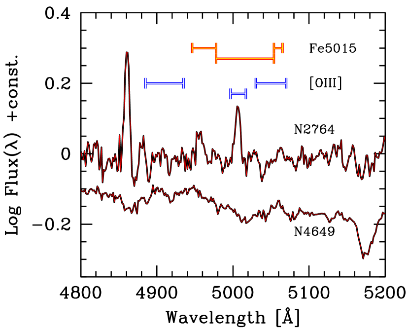
Figure 4: The nested configuration of the [OIII]₅₀₀₇ and Fe5015 indices. For each index the two blue and red pseudo-continuum sideband are reported, flanking the main feature window. Two representative spectra of active (NGC 2764) and quiescent (NGC 4649) elliptical galaxies, from our observed database (Buzzoni et al., 2009b), are superposed to the index sketch, for the sake of comparison. In addition to the [OIII] emission, note for NGC 2764 also a prominent H$\beta$ emission at the nominal $\lambda\lambda\,4861$ Å.

To a closer analysis, things may actually be much more entangled as i) apparent [OIII] emission is partly at odds with Fe5015 absorption, as both indices partly overlap (see Fig. 4); ii) fresh star formation could likely trigger both [OIII] and Balmer emission but on different timescales (Moustakas, Kennicutt, & Tremonti, 2006; Buzzoni et al., 2015), and depending on Oxygen abundance and ionization parameters (Osterbrock, 1974; Pagel et al., 1979; Kewley & Dopita, 2002). For all these reasons, the combined behaviour of the three indices, H$\beta$, [OIII]₅₀₀₇ and Fe5015, needs to be assessed self-consistently.

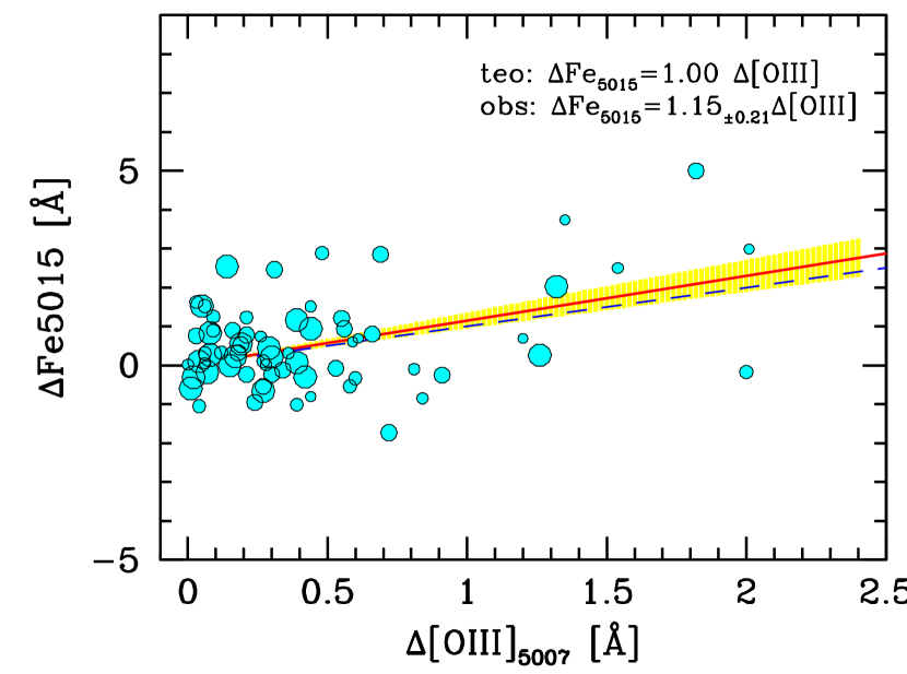
Figure 5: The $\Delta$-$\Delta$ correlation test, as for Fig. 3, for the [OIII]₅₀₀₇ and Fe5015 indices. The expected statistical prediction, according to eq. (28) (dashed line), is well matched by the observations, the latter ones providing a fully consistent $\alpha=1.15_{\pm 0.21}$ fitting line slope (solid line within a $\pm 1\sigma$ yellow fan), as reported top right in the plot.

It is useful to start our analysis first with the [OIII]₅₀₀₇ versus Fe5015 interaction. Figure 4 clearly shows that Oxygen emission may be systematically underestimated as the [OIII]₅₀₀₇ continuum sidebands cannot account for Fe5015 absorption. This is especially true if one considers that Fe5015 strengthens in old stellar systems (Trager et al., 2000; Beuing et al., 2002; Ogando et al., 2008; Buzzoni et al., 2015) (see, for instance, the illustrative case of galaxy NGC 4649, also displayed in Fig. 4). Let us then compute the observed flux density within the [OIII] and Fe5015 feature windows (of width $w_{O}$ and $w_{50}$, respectively).

By recalling eq. (2) and (9), and omitting the “average” overlined notation for flux density symbols, as well as the suffix to the Oxygen index, for better legibility of the formulae, we have

$${f_{O}\over f_{c}}=\big{(}1-{[OIII]\over w_{O}}\big{)},\qquad{f_{50}\over f_{c}}=\big{(}1-{Fe5015\over w_{50}}\big{)}.$$ (22)

Note that $f_{O}$ is in fact a sum of the genuine contribution of O emission plus the contribution of the intrinsic Fe5015 feature. Similarly, the intrinsic Fe5015 flux density (i.e. after fully removing O emission) is

$${f^{\prime}_{50}\over f_{c}}=\big{(}1-{Fe5015^{\prime}\over w_{50}}\big{)},$$ (23)

where Fe5015’ stands for the corrected Fe5015 index strength. By definition, it must be

$$f^{\prime}_{50}(w_{50}-w_{O})=f_{50}\,w_{50}-f_{O}\,w_{O}$$ (24)

so that, after matching eq. (22),

$${f^{\prime}_{50}\over f_{c}}=\Big{[}{{w_{50}\big{(}1-{Fe5015\over w_{50}}\big{)}-w_{O}\big{(}1-{[OIII]\over w_{O}}\big{)}}\over{(w_{50}-w_{O})}}\Big{]}.$$ (25)

When combining eq. (23) and (25) this lead to

$$Fe5015^{\prime}=w_{50}\ \big{(}1-{f^{\prime}_{50}\over f_{c}}\big{)}={w_{50}\over{w_{50}-w_{O}}}\ \big{(}Fe5015-[OIII]\big{)}.$$ (26)

By replacing the corresponding width of each feature window (namely $w_{O}=20$ Å and $w_{50}=76.3$ Å, see Table 1), the intrinsic Fe5015 index can eventually be written explicitely in terms of the observed quantities as

$$Fe5015^{\prime}=1.36\ \big{(}Fe5015-[OIII]\big{)}.$$ (27)

As far as the $\Delta$-$\Delta$ index distribution is concerned, if the same (intrinsic) value of Fe5015’ has to be expected in the galaxy “left” and “right” side, at fixed radial distances, then any difference in the observed Fe5015 index may be induced by a change in the [OIII] emission. By simply differentiating eq. (27), we obtain a straight positive correlation such as

$$\Delta Fe5015=\Delta[OIII].$$ (28)

Again, when comparing in Fig. 5 with our data, a least-square solution on 68 selected points in total (after a $3\sigma$ clipping) provides a fully consistent slope value $\alpha=1.15_{\pm 0.21}$.

Quite importantly, turning back for a moment to eq. (27), one has to notice that, when [OIII] emission fades and Fe5015 tends to Fe5015’, then the [OIII] index does not vanish. In fact, if we set $Fe5015=Fe5015^{\prime}$ in eq. (26), one obtains

$$[OIII]_{\rm min}={w_{O}\over w_{50}}Fe5015^{\prime}=0.26\ Fe5015^{\prime}$$ (29)

More generally, if some emission occurs, then $[OIII]^{\prime}=[OIII]-[OIII]_{\rm min}$, and

$$[OIII]^{\prime}=[OIII]-0.26\ Fe5015^{\prime},$$ (30)

or

$$[OIII]^{\prime}=1.36\ [OIII]-0.36\ Fe5015$$ (31)

putting it in terms of the observed quantities. Equation (30) gives the locus in the Fe5015 versus [OIII] plane for any intrinsic emission strength $[OIII]^{\prime}$.

By combining eq. (26) and (30), an obvious self-consistency constraint implies that

$$Fe5015^{\prime}=Fe5015-[OIII]^{\prime}.$$ (32)

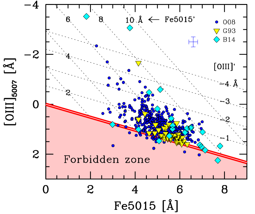
Figure 6: The observed (raw) [OIII]₅₀₀₇ versus Fe5015 index distribution for the Ogando et al. (2008) (solid dots), González (1993) (triangles) and (Buzzoni et al., 2009b, 2015) (rombs) samples of early-type galaxies. The forbidden zone in the index domain is shaded, according to eq. (31), while a more general parameterization versus intrinsic Fe5015 and [OIII]₅₀₀₇ strength (primed indices in the plot) is displayed, in force of eq. (27) and (31). An indicative error box for the observations is reported top right.

A graphical summary of our theoretical scheme is sketched in Fig. 6, where we compare the [OIII] versus Fe5015 distribution for the galaxies of Table 2 with the observed distribution of an extended sample of 509 ellipticals from Ogando et al. (2008) and with the González’ (1993) original bulk of 41 ellipticals. The trend seems quite encouraging, and actually calls for an important property of ellipticals. Within the limits of Ogando’s et al. (2008) calibration (see in particular Table 7 and 8 therein), in fact, these data indicate that a substantial fraction of galaxies displays some residual Oxygen emission (Sarzi et al., 2006; Papaderos et al., 2013). This important issue can be better assessed by means of Fig. 7, where we derive the distribution of the intrinsic emission $[OIII]^{\prime}$ as from eq. (31) The whole sample of 498 galaxies with available Fe5015 and [OIII]₅₀₀₇ indices leads to a mean index strength $\langle{[OIII]^{\prime}}\rangle=-0.70\pm 0.54$ Å, with an evident skewness toward enhanced [OIII] emissions. Just as a reference, 16 objects out of 498 (3%) in the figure display an intrinsic [OIII] feature stronger than 2 Å, while for 107 galaxies (21%) the [OIII] emission exceeds 1 Å.

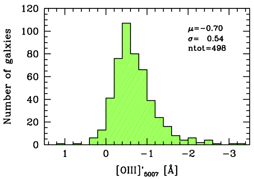
Figure 7: The [OIII]₅₀₀₇ distribution of the intrinsic (“primed”) index among the Ogando et al. (2008) early-type galaxy sample. A total of 498 galaxies, with available [OIII]₅₀₀₇ and Fe5015 observations are displayed. The [OIII] observations have been corrected according to eq. (31). On average, ellipticals display a weak residual gas emission with $\langle[OIII]^{\prime}_{5007}\rangle=-0.70_{\pm 0.54}$ Å. For a fraction of 21% of the total sample, the intrinsic [OIII] pseudo-equivalent width is in excess of 1 Å, while about 1/7 of these galaxies (16 out of 498) display a striking (star-formation) activity, with [OIII]’${}_{5007}\la-2$ Å.

After disentangling the combined behaviour of [OIII] emission and Fe5015 absorption, we are now in a better position to tune up an H$\beta$ correction scheme. Again, our $\Delta$-$\Delta$ diagnostic plot may add useful hints to tackle the problem. The rationale, in this case, is that the observed $\Delta[OIII]_{5007}$ should directly trace the corresponding [OIII]’ intrinsic change, via eq. (30), providing the Fe5015’ strength is the same at symmetric distances from the galaxy center. We could therefore probe the $\Delta H\beta$ data set for any possible correlation with the corresponding $\Delta[OIII]_{5007}$ output in a fully empirical way.

For this task, we divided the whole galaxy set of Table 2 (Sample “A”) in different subsamples according to the “activity level” as traced by the overall spectral characteristics. In particular, we considered three refence samples. Sample “B” consists of the 7 “quiescent” galaxies with no reported emission lines. Sample “C” includes, on the contrary, the 8 “moderately active” objects, marked with one asterisk in the table, wich are reportedly emitting at least the [OII] 3727 Å feature. Finally, the 5 “most active” ellipticals (that is those marked with double asterisk in Table 2) are included in Sample “D”. They display [OII] 3727 Å emission accompanied by the strongest [OIII]’ index in Fig. 6. Our results are summarized in the four panels of Fig. 8. As usual, the fitting slope after $3\sigma$ data clipping is presented in Table 3 together with the mean of central corrected [OIII] emission, (as from Buzzoni et al., 2015).

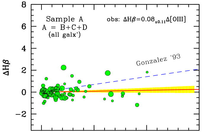
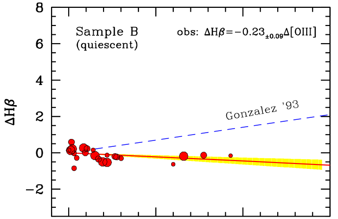
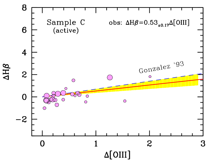
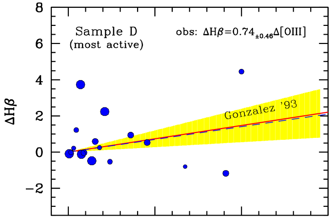
Figure 8: The $\Delta$-$\Delta$ correlation test, as for Fig. 3, for the [OIII]₅₀₀₇ and H$\beta$ indices in the adopted Buzzoni et al. (2009b, 2015) sample of early-type galaxies. The whole Sample A, of the 20 objects (upper panel), is split into three groups (i.e. Samples “B”, “C” and “D”, from top to bottom) consisting, respectively of 7, 8, and 5 galaxies with increasing gas emission activity. Groups have been assembled according to the asterisk ranking of Table 1, that combines the Bettoni & Buson (1987) empirical classification with the [OIII] index strength in our observations. The dashed line, in each plot, marks the González (1993) $\Delta$-$\Delta$ correction slope. Our least-square fit is reported top right in each panel, and displayed (solid line) together with its corresponding $\pm 1\sigma$ uncertainty (yellow fan). Our output is summarized in Table 3.

Table 3: Core [OIII]’ emission strength and observed $\Delta H\beta$ versus $\Delta[OIII]$ fitting slope

Sample	$\langle$[OIII]’$\rangle^{\dagger}$	$\alpha$	n‡
A - All galaxies (20 obj)	–1.1	0.08	(68)
	$\pm 1.7$	$\pm 11$
B - Quiescent only (7 obj)	–0.15	–0.23	(23)
	$~{}\pm 74$	$\pm 9$
C - Interm. active (8 obj)	–0.67	0.53	(25)
	$~{}\pm 49$	$\pm 17$
D - Most active (5 obj)	–3.1	0.74	(17)
	$\pm 2.3$	$\pm 46$
† Mean core [OIII]’ index, in Å, as from Buzzoni et al. (2015)
‡ Number of available pairs of points in the $\alpha$ fit

A firm important conclusion of our analysis, is that no striking correlation seems in place across the whole galaxy sample between H$\beta$ and [OIII]₅₀₀₇. A mild positive slope is found overall (Sample “A”, upper left panel in Fig. 8), only marginally in excess to the flat-slope case ($\alpha=0.0$-0.2). The flattening effect is clearly induced by the fraction of “quiescent” ellipticals (Sample “B”, upper right panel), for which we even notice a slight anti-correlation ($\alpha\sim-0.2$). However, with increasing stellar activity, as in Sample “C” and “D” galaxies, one has to notice some hints of a change. Although with increased scatter and a much blurred trend, the data seem to point to a steeper slope $\alpha$ and, at least for Sample “D” (lower left panel in the figure), our results nominally match González’ (1993) value.

As a plain “thumb rule”, we could state that González’ (1993) correction scheme fully holds for the most active strong-lined ellipticals, where $[OIII]^{\prime}$ emission roughly exceeds 2 Å. For intermediate cases (say for [OIII]’ emission strength about 1 Å) a flatter slope ($\alpha\sim 0.3$-0.5) might be more appropriate, while a negligible H$\beta$ correction ($\alpha\sim 0.1$) is required for weaker [OIII] emission. As shown in Fig. 9, a logistic curve could be adopted as a convenient analytical fit of this scheme, such as

$$\alpha={{0.75}\over{1+e^{k}}},$$ (33)

with $k=([OIII]^{\prime}+1)/0.25$, and [OIII] emission assumes, of course, negative values. The corrected H$\beta$ index therefore derives as

$$H\beta_{\rm corr}=H\beta_{\rm obs}-H\beta_{e}=H\beta_{\rm obs}-\alpha\,[OIII]^{\prime}.$$ (34)

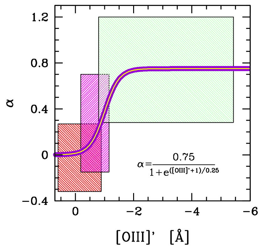
Figure 9: The devised correction scheme for H$\beta$ in the form of a logistic curve versus intrinsic [OIII]’ emission, as from eq. (33). The “quiescent”, “active” and “most active” galaxy samples of Fig. 8 are sketched by the three shaded boxes, with [OIII]’ mean central values and $\alpha$ error bars as from Table 3.

3.3 Mg₁ + Mgb = Mg₂?

The prominent Magnesium feature about 5200 Å is by far the most popular target in optical spectroscopy of elliptical galaxies and other old stellar systems. As explored in full detail by Mould (1978), from a theoretical point of view, this feature is in fact a blend of both the atomic contribution of the Mgb triplet at 5178 Å, and the (1,1) $A^{2}\Pi\ X^{2}\Sigma^{+}$ vibrational band head of the MgH molecule. This transition of Magnesium Hydride has a dissociation energy of 1.34 eV (Coelho et al., 2005, as from Huber & Herzberg, 1979 data), a much lower threshold than the first-ionization potential of 7.65 eV for atomic Mg. As a consequence, the Mgb absorption tends to be the prevailing one in warmer (type F-G) stars, while it accompanies the surging MgH absorption at the much cooler temperature regime of K-M stars. In addition, the relatively more flimsy structure of the molecule makes MgH very sensitive to stellar luminosity class (Buzzoni et al., 2001), as gravity acts on electron pressure of the stellar plasma and slightly modulate the dissociation energy threshold. This dependence, however, is severely tackled by the intervening appearence of TiO bands among M-type stars, which substantially affect the pseudo-continuum level (Tantalo & Chiosi, 2004; Buzzoni, Gariboldi, & Mantegazza, 1992, see, for instance Fig. 5 therein).

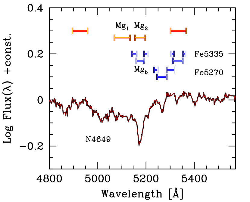
Figure 10: An illustrative sketch of the Mg index set, and the two Fe5270 and Fe5335 indices. For each index, the blue and red sidebands are marked, flanking the relevant feature window. The nested configuration of the Mgb, Fe5335 and Mg₂ indices is well evident, as discussed in the text. The representative spectrum of the elliptical galaxy NGC 4649 (from the Buzzoni et al., 2009b, data) is superposed for the sake of comparison.

The Magnesium complex is sampled by three Lick indices, namely Mg₁, Mg₂, and Mgb. The strategy is for Mg₂ to somewhat bridge the other two, with Mg₁ especially suited to probe the molecular contribution, and the Mgb index better tuned on the atomic triplet (see Fig. 10). Within this configuration, Mg₂ shares its feature window with Mgb, and its pseudo-continuum windows with the Mg₁ index. From its side, Mgb aims at recovering the genuine atomic contribution by setting its pseudo-continuum level about the Mg₁ bottom (see again Fig. 10 for an immediate sketch).

Similarly to what discussed in previous section, we can further expand our scheme to assess in a more straightforward way the Mg₂-Mgb-Mg₁ index entanglement. First of all, as both Mg₂ and Mg₁ are expressed in magnitudes and Mgb in Å, it is convenient to recall the basic relations of eq. (3) and (4) and write

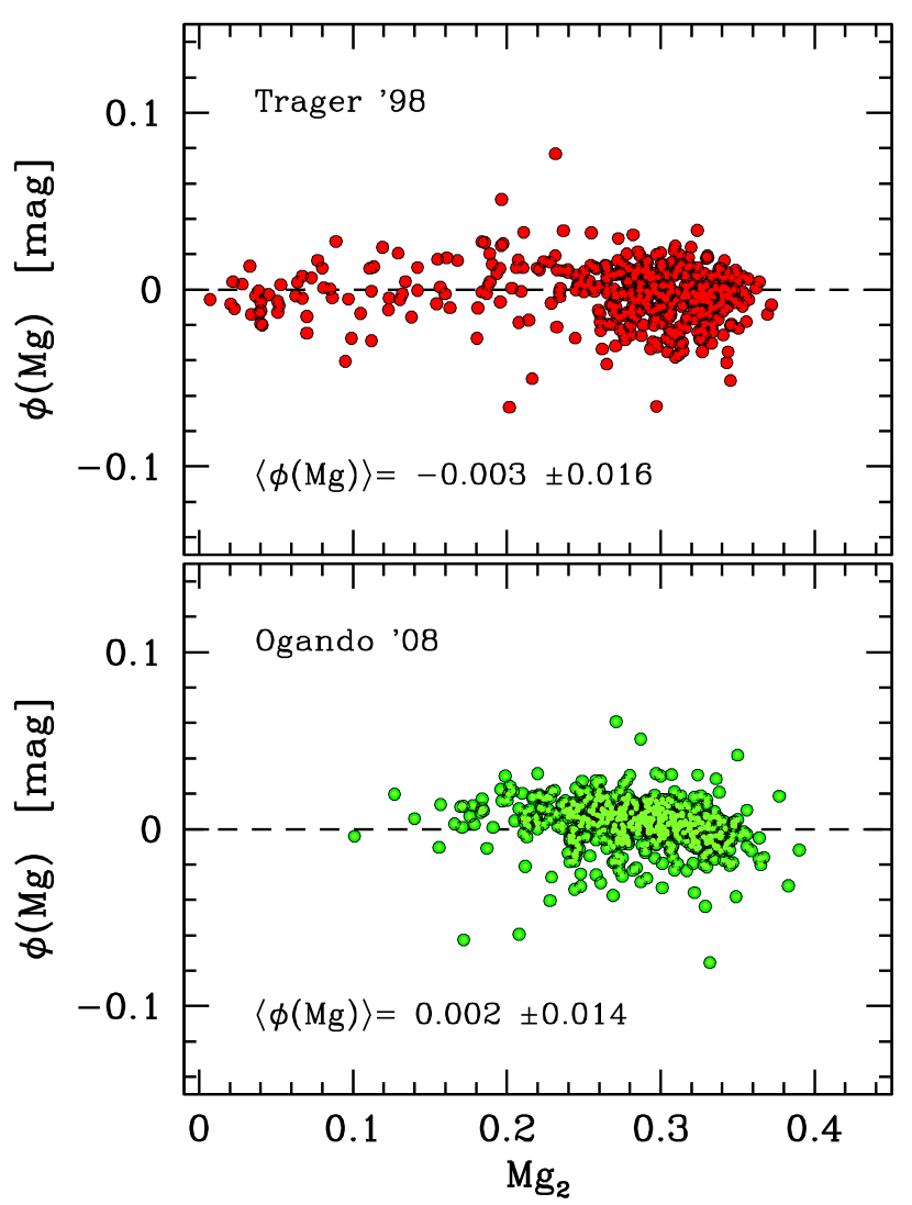
Figure 11: An empirical check of the expected relationship among the three popular Mg indices sampled by the Lick system. The synthesis function $\phi(Mg)$ of eq. (44) has been scrutinized by means of the two extended early-type galaxy samples of Trager et al. (1998) (406 galaxies with complete Mg₁, Mg₂ and Mgb data, see upper panel), and Ogando et al. (2008) (481 galaxies, lower panel). The match with both samples allowed us to obtain the fine-tuning offset in the theoretical relationship, such as $k=0.03$ mag. After offset application, notice for both plots the lack of any drift in the point distribution, a feature that assures the correct parameterization of our theoretical relationship. In addition, the point scatter around the zero line indicates that index mutual relationship can be obtained within a $\sim$1.5% internal accuracy.

$$\left\{\begin{array}[]{lcl}{f_{2}/f_{c}}&=&10^{-0.4\,\mathrm{Mg}_{2}}\\ \\ {f_{1}/f_{c}}&=&10^{-0.4\,\mathrm{Mg}_{1}}\\ \\ {f_{b}/f_{1}}&=&\left(1-{{\rm Mgb}/w_{b}}\right).\end{array}\right.$$ (40)

We can also combine the last two equations above to obtain

$${f_{b}\over f_{c}}=\left({f_{b}\over f_{1}}\right)\left({f_{1}\over f_{c}}\right)=\left(1-{{\rm Mgb}\over w_{b}}\right)\,10^{-0.4\,{\rm Mg}_{1}}.$$ (41)

Quantities $f_{2},f_{1}$, and $f_{b}$ in previous equations refer to the flux density of Mg₂, Mg₁ and Mgb feature windows, respectively, and $w_{b}$ is the width of the Mgb feature window. For Mg₁ and Mg₂ this flux is normalized to the same pseudo-continuum, f_c, while the f₁ bottom level can also be seen as a proxy of the Mgb pseudo-continuum.

Likewise eq. (24), also for the Mg case we can write

$$f_{2}\,w_{2}=f_{1}\,(w_{2}-w_{b})+\left({f_{b}\over f_{1}}\right)\,f_{1}\,w_{b},$$ (42)

being $w_{2}=42.5$ Å and $w_{b}=32.5$ Å (from Table 1) the width of the Mg₂ and Mgb feature windows, respectively. By matching eq. (40), (41) and (42) and taking the logarithm, after little arithmetic, we lead to the final form that links the three indices:

$${\rm Mg}_{2}-{\rm Mg}_{1}=-2.5\,\log\left(1-{{\rm Mgb}\over w_{2}}\right)+k.$$ (43)

In the equation we left a fine-tuning offset ($k$) in order to account for the little aproximation we made in eq. (40) for f₁ to be an exact proxy of the Mgb pseudo-continuum level. It is interesting to verify, on empirical basis, the invariancy of the function

$$\phi({\rm Mg})={\rm Mg}_{2}-{\rm Mg}_{1}+2.5\,\log\left(1-{{\rm Mgb}\over w_{2}}\right)-k.$$ (44)

Again, the Ogando et al. (2008) together with the Trager et al. (1998) galaxy database provide us with an excellent reference tool. Our results are summarized in the two panels of Fig. 11. As predicted, the lack of any drift of $\phi({\rm Mg})$ versus Mg₂ (and versus Mg₁ and Mgb, as well) indicates that no residual dependency has been left unaccounted in our analysis. By searching the least-square fit to the data, we also get an empirical estimate for the fine-tuning offset, that is $k=0.03$ mag. Providing to observe two indices, eq. (43) allows us to secure the third one within a $\sim 1.5$% internal accuracy.

A further check can be carried out in terms of our $\Delta$-$\Delta$ test. By differentiating eq. (43), and considering that, in general, Mgb $\ll w_{2}$, we obtain, in fact

$$d{\rm Mg}_{2}-d{\rm Mg}_{1}\simeq{1\over w_{2}}\,{d{\rm Mgb}\over(1-{\rm Mgb}/w_{2})}\approx 0.024\,d{\rm Mgb},$$ (45)

The thoretical relationship is probed in Fig. 12 with our galaxy sample of Table 2. The usual least-square fit procedure to a total of 66 points provides a value of the slope $\alpha=0.019_{\pm 0.003}$.

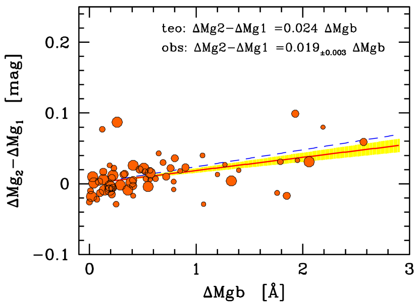
Figure 12: The $\Delta$-$\Delta$ correlation test, as for Fig. 3, for the Mg index complex. The $\Delta Mg_{1}$, $\Delta Mg_{2}$ and $\Delta$ Mgb variation across the Buzzoni et al. (2009b, 2015) galaxy sample of Table 2 is probed in terms of the expected relationsip, as from eq.(45) (dashed line in the plot). Our least-square fit is reported top right, and displayed (solid line) together with its corresponding $\pm 1\sigma$ statistical uncertainty (yellow fan).

3.3.1 The [NI]₅₁₉₉ hidden bias

As for the case of the [OIII]₅₀₀₇ perturbing emission to the Fe5015 index, also for the Mgb index one may expect a shifty, and mostly neglected, bias from overlapping gaseous emission lines. This is the case of the [NI] forbidden doublet at 5198/5200 Å (hereafter [NI]₅₁₉₉), a somewhat ominous weak feature that characterizes the spectra of LINER galaxies (Osterbrock, 1974, see Appendix 4 therein), including ellipticals, either due to residual star formation activity (Sarzi et al., 2006; Cappellari et al., 2011), or simply supplied by the post-AGB stellar component (Kaler, 1980; Ferland et al., 2012; Kehrig et al., 2012; Papaderos et al., 2013).

Goudfrooij & Emsellem (1996) have been discussing in some detail the perturbing effect of [NI]₅₁₉₉ on the computed Mgb index in the spectra of elliptical galaxies. Differently from the [OIII]₅₀₀₇ versus Fe5015 interplay, the [NI]₅₁₉₉ emission positively correlates with the affected Mgb as [NI] luminosity enhances the pseudo-continuum level in the red side band of Mgb (see Fig. 10), thus leading to a stronger index.

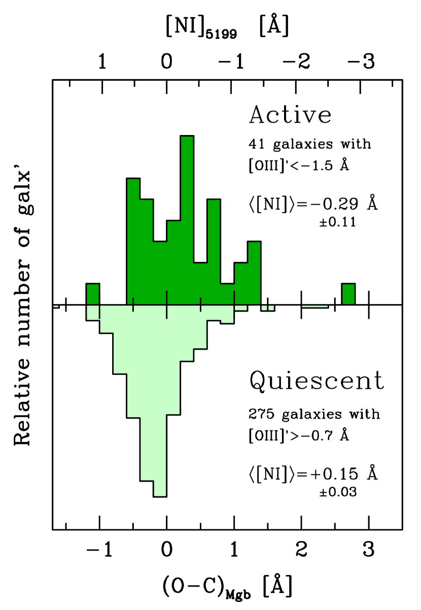
Figure 13: The inferred distribution of the “hidden” [NI]₅₁₉₉ gas emission in the Ogando et al. (2008) galaxy sample. In case of intervening [NI] emission, the Mgb index is expected to enhance, on average, by the amount of eq. (48) with respect to its theoretical figure, as from eq. (43). This excess (in the sense “Observed – Computed”, see lower x axis), and the related [NI] strength (upper x axis) is probed by contrasting the subsample of 41 “active” galaxies (as traced by explicit [OIII] emission stronger than 1.5 Å, as in the upper histogram) with the population of 275 “quiescent” galaxies with vanishing [OIII] (see the lower histogram). See text for a discussion.

A simple correction scheme can be devised, to size up the [NI]₅₁₉₉ bias just relying on the third relation of eq. (40) (and, again, assuming $f_{1}$ as the reference Mgb pseudo-continuum flux density). By passing to logarithms we have:

$$\ln\left(1-{{\rm Mgb}\over w_{b}}\right)=\ln(f_{b})-\ln(f_{1})$$ (46)

Again, considering that Mgb $\ll w_{b}$, the l.h. term of the equation can be approximated by $-({\rm Mgb}/w_{b})$ so that, by differentiating with respect to f₁, we have

$${d{\rm Mgb}\over w_{b}}\simeq{df_{1}\over f_{1}}.$$ (47)

If [NI]₅₁₉₉ emission appears, then a supplementary flux F_N is added to the Mgb pseudo-continuum, and its reference flux density changes by $df_{1}=F_{N}/W_{b}$, where $W_{b}=33.7$ Å, as from Table 1. As, by definition, the [NI] equivalent width is $[NI]_{5199}\simeq-{F_{N}/f_{1}}$, eq. (47) can eventually be re-arranged in its final form

$${\rm dMgb}=-[NI]_{5199}\left(w_{b}\over W_{b}\right)\simeq-0.96\,[NI]_{5199}.$$ (48)

Our result nicely compares with Goudfrooij & Emsellem (1996), who led to a more crude analytical estimate of the effect such as ${\rm dMgb}\simeq-1.1\,[NI]_{5199}$.

The Ogando et al. (2008) extended galaxy database allows us a further independennt assessment of the [NI]₅₁₉₉ bias among elliptical galaxies. In this regard, we set up a simple test aimed at comparing the observed Mgb index for the entire galaxy dataset with the corresponding “predicted” output as from eq. (43). Galaxies with intervening [NI] emission are expected to display (on average) a stronger-than-predicted Mgb index, and one could envisage to detect this signature in the index (O-C) (i.e. “observed - computed”) residual distribution.

In order to get a cleaner piece of information, we only restrained our analysis to the galaxy sub-sample with stronger and poorer [OIII]₅₀₀₇ emission, assuming [OIII]₅₀₀₇ to be also a confident proxy for [NI]₅₁₉₉ activity (Osterbrock, 1974). According to the [OIII]’₅₀₀₇ distribution of Fig. 7, we therefore selected a sample of 41 “active” galaxies with [OIII]’${}_{5007}<-1.5$ Å emission, to be compared with a group of 275 objects with average or less-than-average (i.e. [OIII]’${}_{5007}>-0.7$ Å) emission. For each galaxy with observed Mg₂ and Mg₁ indices we then computed the corresponding Mgb, via eq. (43) (by setting $k=0.03$ therein), and compared it with the observed entry in the catalog. The output distribution for the “active” and “quiescent” galaxy samples is displayed in Fig. 13. According to eq. (48), the (O-C) residuals have been directly converted into a fiducial [NI]₅₁₉₉ emission strength, as in the upper x-axis scale of the figure. Within the uncertainty of our theoretical procedure, just a glance to Fig. 13 confirms the lack of any [NI] emission among “quiescent” galaxies ($\langle[NI]_{5199}\rangle=+0.15$$\pm 0.03$ Å, on average), while a weak but significant ($>3\sigma$) activity has to be reported, on the contrary for “active” systems, with $\langle[NI]_{5199}\rangle=-0.29$$\pm 0.11$ Å. Interestingly enough, the [NI]/[OIII] $\sim 0.3/1.5$ observed ratio for the “active” sub-sample matches in the right sense the corresponding empirical figure for the LINER galaxies, as suggested by Goudfrooij & Emsellem (1996, see Table 1 therein).

3.4 Spectral duality: the case of Fe5335

Due to wavelength oversampling, along the Lick-index sequence it may even happen that individual spectral features are accounted twice being also included in some pseudo-continuum windows of other indices. One relevant case, in this sense, is the Fe5335 index, which is fully comprised inside the (red) pseudo-continuum window of both the Mg₂ and Mg₁ indices. In addition, it also entirely shares its own red pseudo-continuum with the blue side-window of Fe5270 (see, again, Fig. 10). Evidently, this makes both the Fe5270 and the Mg indices to somewhat correlate with the Fe5335 strength. To explore this effect let us start first with the simpler case of Fe5335-Fe5270 entanglement.

According to Table 1, the Fe5270 pseudo-continuum is sampled along a total of 47.5 Å (i.e. red+blue side-windows, $W_{52}$), whose 11.3 Å are shared with the Fe5335 red side-band ($W_{53}^{\rm red}$). The total side-windows for Fe5335 (i.e. $W_{53}=W_{53}^{\rm red}+W_{53}^{\rm blue}$) amount to 21.2 Å, and both features are sampled within similar wavelength windows ($w_{52}$ and $w_{53}$) of 40 Å each. By recalling eq. (2) and passing to logarithm, for Fe5270 we have

$$\ln\left(1-{Fe5270\over w_{52}}\right)=\ln(f_{52})-\ln(f_{52}^{c}).$$ (49)

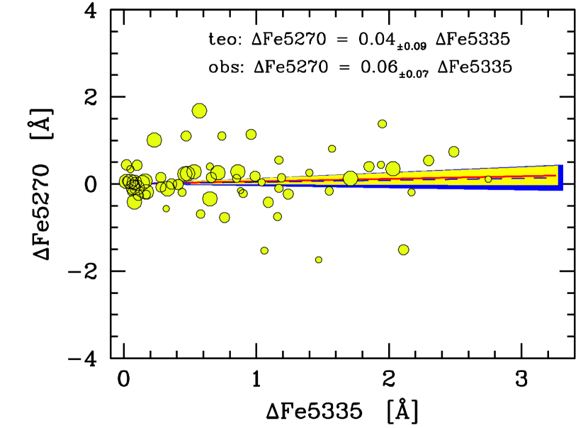
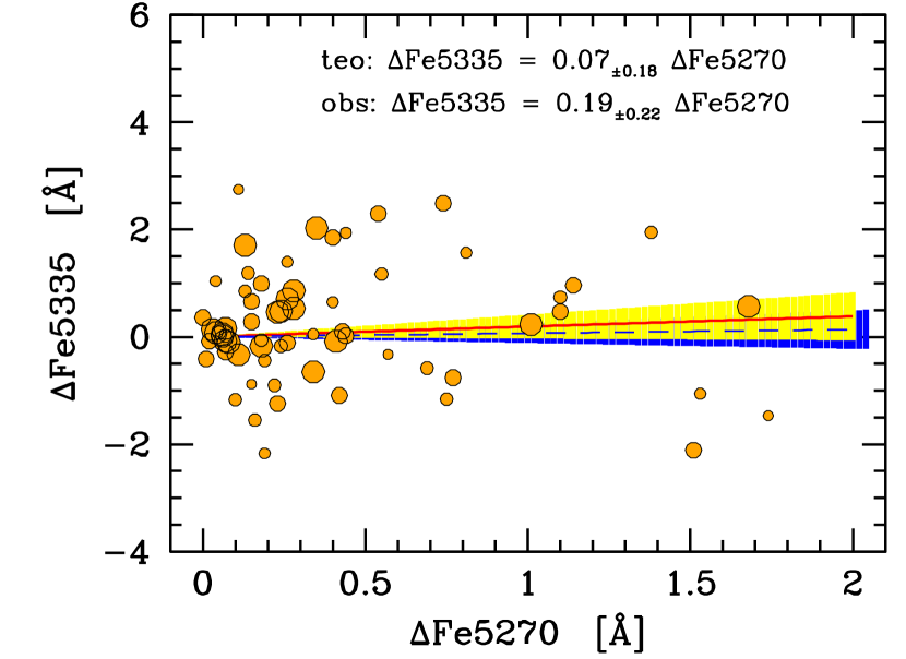
Figure 14: The $\Delta$-$\Delta$ correlation test, as for Fig. 3, for the Fe5270 and Fe5335 indices. The low correlation between index variation, as predicted by eq. (53) and (56) (dashed lines in the two plots, with their corresponding $\pm 1\sigma$ Bayesian uncertainties, as from the blue fans) is consistently resumed by our observing test on the galaxy sample of Table 2 (solid lines with their corresponding $\pm 1\sigma$ statistical uncertainties, as from the yellow fans). See text for a discussion.

As we are dealing with a weak absorption line (so that $Fe5270/w_{52}\ll 1$) the l.h. term of the equation can be approximated by $-(Fe5270/w_{52})$. By differentiating,

$$\big{(}{dFe5270\over w_{52}})={df_{52}^{c}\over f_{52}^{c}}-{df_{52}\over f_{52}}.$$ (50)

A similar notation holds for Fe5335, too. Any change (for whatever reason) in the $f_{53}^{c}$ flux density, would therefore reverberate into a change in the Fe5270 and Fe5335 strengths as well, so that

$$\big{(}{dFe5270\over w_{52}}\big{)}={df_{52}^{c}\over f_{52}^{c}}\sim{df_{53}^{c}\over f_{53}^{c}}{W_{53}^{\rm red}\over W_{52}}\sim\big{(}{dFe5335\over w_{53}}\big{)}\big{(}{W_{53}^{\rm red}\over W_{52}}\big{)},$$ (51)

or

$$dFe5270=\big{(}{11.3\over 47.5}\big{)}\,dFe5335=0.238\,dFe5335.$$ (52)

The chance for Fe5335 to entangle Fe5270 depends on the probability for any random change in the Fe5335 index bands to affect the wavelength range in common with the Fe5270 pseudo-continuum. This can be be estimated of the order of $W_{53}^{\rm red}/(W_{53}+w_{53})\sim 11.3/61.2=18$% being, therefore, 82% the probability for no entanglment at all between the two indices. By accounting for these figures, the average expected relationship between Fe5270 and Fe5335 eventually results in

$$\begin{array}[]{rl}dFe5270&=(0.238\times 0.18)+(0\times 0.82)\,dFe5335\\ &=0.043_{\pm 0.091}\,dFe5335.\\ \end{array}$$ (53)

This value has to be compared with the $\Delta$-$\Delta$ test as displayed in the upper panel of Fig. 14. From our data (66 points in total) we obtain $\alpha=0.059_{\pm 0.068}$.

Quite importantly, note that eq. (53) cannot be simply reversed, once considering the impact of the overlapping window on the Fe5335 strength (because $W_{53}\neq W_{52}$). By reversing the indices in eq. (51), in fact we have

$$\big{(}{dFe5335\over w_{53}}\big{)}={df_{53}^{c}\over f_{53}^{c}}\sim{df_{52}^{c}\over f_{52}^{c}}{W_{53}^{\rm red}\over W_{53}}\sim\big{(}{dFe5270\over w_{52}}\big{)}\big{(}{W_{53}^{\rm red}\over W_{53}}\big{)},$$ (54)

or

$$dFe5335=\big{(}{11.3\over 21.2}\big{)}\,dFe5270=0.533\,dFe5270.$$ (55)

This interaction has a probability of the order of $W_{53}^{\rm red}/(W_{52}+w_{52})\sim 11.3/87.5=13$%. so that, similar to eq. (53), the eventual relationship, by reversing the indices in a $\Delta$-$\Delta$ test becomes

$$\begin{array}[]{rl}dFe5335&=(0.533\times 0.13)+(0\times 0.87)\,dFe5270\\ &=0.07_{\pm 0.18}\,dFe5270.\end{array}$$ (56)

Again, this relationship can be probed by means of our $\Delta$-$\Delta$ test, as shown in the lower panel of Fig. 14, suggesting $\alpha=0.19_{\pm 0.22}$.

As far as the Mg₂- (or Mg₁-) Fe5335 entanglement is concerned, we can proceed in a similar way, depending whether a change occurs in the feature or in the side-band windows of the FeI index. According to Table 1, the Mg₂ (or Mg₁) pseudo-continuum is sampled along a total of $W_{2}=127.5$ Å. Of these, 40 Å and 21.2 Å are shared, respectively, with the feature ($w_{53}$) and the side bands ($W_{53}$) of the Fe5335 index.

By recalling that Mg₂ (and Mg₁) are expressed in magnitude, the equivalent of previous eq. (51), in case of an intervening change in the Fe5335 pseudo-continuum flux, becomes

$$d{\rm Mg}_{2}\sim{df_{2}^{c}\over f_{2}^{c}}\sim{df_{53}^{c}\over f_{53}^{c}}{W_{53}\over W_{2}}\sim\big{(}{dFe5335\over w_{53}}\big{)}\big{(}{W_{53}\over W_{2}}\big{)},$$ (57)

which leads to

$$d{\rm Mg}_{2}=\big{(}{21.2\over 40\times 127.5}\big{)}\,dFe5335=+0.0042\,dFe5335.\\$$ (58)

This outcome has a probability of the order of $W_{53}/(W_{53}+w_{53})\sim 21.2/61.2=35$%.

On the other hand, any change in the Fe5335 feature window will affect the Mg₂ (Mg₁) strength by

$$d{\rm Mg}_{2}\sim{df_{2}^{c}\over f_{2}^{c}}\sim{df_{53}\over f_{53}}{w_{53}\over W_{2}}\sim-\big{(}{dFe5335\over w_{53}}\big{)}\big{(}{w_{53}\over W_{2}}\big{)}.$$ (59)

By replacing the relevant quantities, in this case we have

$$d{\rm Mg}_{2}=-\big{(}{1\over 127.5}\big{)}\,dFe5335=-0.0078\,dFe5335,$$ (60)

with a probability of $w_{53}/(W_{53}+w_{53})\sim 40/61.2=65$%. Therefore, if a random process (of whatever origin) is at work by changing Fe5335, then the weighted average of eq. (58) and (60) eventually provides us with the expected relationship for Mg₂ (and similarly, for Mg₁, as well):

$$dMg_{2}=dMg_{1}=-0.0036_{\pm 0.0057}\,dFe5335.\\$$ (61)

Our theoretical output is probed in Fig. 15, by averaging the $\Delta$Mg₁ and $\Delta$Mg₂ versus $\Delta$Fe5335 variations for a cleaner display of the effect. Observations actually confirm the nearly vanishing relationship in place across the whole galaxy sample, making the expected impact of Fe5335 random change on Mg indices negligible.

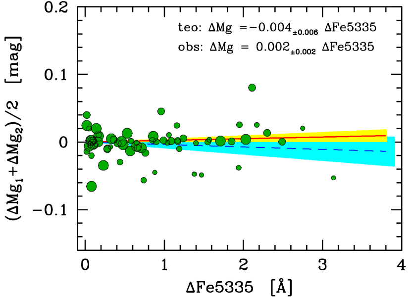
Figure 15: The $\Delta$-$\Delta$ correlation test, as for Fig. 3, for the Fe5335 and Mg indices. The observed relationship for Mg₁ and Mg₂ is averaged, to gain a cleaner view of the effect. In spite of the average low correlation, as predicted by eq. (61) (dashed line) one has to notice the important Bayesian uncertainty (blue fan in the plot, tracing the $\pm 1\sigma$ uncertainty), which makes the bias effect of Mg-Fe5335 entanglement possibly of non-negligible impact on individual galaxies.

On the other hand, if a change in the Fe5335 feature occurs as a result of a genuine (selective) variation of Fe abundance, then only eq. (60) has to be taken as a reference. Although small, the induced bias on Mg₂ (and Mg₁) may be an issue in this case, expecially if we aim at carefully investigating the [$\alpha$/Fe] ratio in a galaxy sample. In fact, any stronger Fe5335 index would induce, by itself, a shallower Mg index.

3.5 Mr. Iron, I suppose…

About half of the total Lick indices are meant to trace Iron as a main elemental contributor to the index feature. The ominous presence of weak (i.e. non-saturated) absorption lines of FeI and FeII in the optical/UV wavelength region is, of course, a well established property of stellar spectra (e.g. Pagel, 1997), that can be exploited by high-res spectroscopy to set up the linear branch of the spectral curve of growth, thus leading to an accurate measure of the elemental abundance. This figure is usually taken as an empirical proxy of stellar “metallicity”, at large, assuming Iron to scale according to all the other metals. On the same line, also UBV broad-band photometry may rely on the “blanketing” effect, mainly driven by the Iron contribution, to constrain stellar metallicity (e.g. Sandage, 1969; Golay, 1974).

As far as low-res spectroscopy or narrow-band photometry is concerned, as for the Lick indices, however, such a huge number of low-strength Fe lines may reveal a quite tricky feature, as Iron markers actually come heavily blended with other elements. The potential drawback has already been emphasized, at least in a qualitative way, in earlier works dealing with the Lick-system assessment (Burstein et al., 1984; Faber et al., 1985; Gorgas et al., 1993; Worthey et al., 1994, among others). This analysis has then been further carried on by Tripicco & Bell (1995); Worthey (1996); Trager et al. (1998), and Serven, Worthey, & Briley (2005), urging in some cases a revision of the index label, as for the original Fe4668 index (Worthey, 1996; Trager et al., 1998), now redefined as C₂4668 according to the real prevailing contribution in the evolutionary context of old stellar populations, as in elliptical galaxies.

The Trager et al. (1998) revision process has been intentionally left at the highest conservative level, likely to avoid any massive re-definition of the original index set. However, we want to retake here some arguments of Worthey’s (1996) preliminary analysis to show that, at least for some relevant cases dealing with bona fide Fe features, an important update effort seems yet to impose. We will defer this delicate task to a forthcoming paper discussing here, just as an illustrative excercise, the case of index Fe4531.

3.5.1 Absolute and net index sensitivity

The main rationale for Lick-index set up (Worthey et al., 1994) aims at catching all the prominent absorption features in the optical spectra of late-type (type G-K) stars. This uniquely requires the feature to be easily recognized at a $\sim 8.5$ Å (FWHM) resolving power. If a blend could be envisaged for a feature, the latter is tacitly assumed to be named after the element contributing with the deepest line, as recognized from the list of theoretical atomic transitions (e.g. Smith et al., 1996; Piskunov et al., 1995; Kupka et al., 1999). The deepest line also defines the feature centroid, which is reported in the Worthey et al. (1994) original Table 1. No special requirement is demanded to the two index side-bands, set to sample a nearby pseudo-continuum, other than being suitably “feature-free” and sufficiently extended in wavelength such as to be insensitive to stellar velocity dispersion broadening (Worthey et al., 1994).

So, while the main focus is on the feature prominence, that is on feature’s absolute sensitivity to the “leading” chemical element, one should not neglect the fact that it is the index “net” sensitivity (that is by netting the feature sensitivity to a given element with the impact of the latter on the pseudo-continuum bands, too) that eventually set the real index response to a given chemical species.

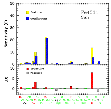
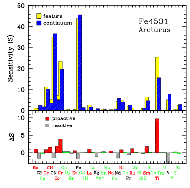
Figure 16: The Fe4531 index sensitivity to the 40 most prominent chemical elements (as sequenced in the x axis, disregarding their ionization states) in the Sun (left panel) and Arcturus (right panel) spectrum. In both panels, the yellow histograms refer to the elemental contribution (${\cal S}^{f}_{X}$) to the feature window, according to the definition of eq. (62), while the blue histograms are for the elemental contribution (${\cal S}^{c}_{X}$) to the flanking pseudo-continuum index sidebands, according to eq. (63). The net contribution to the index strength ($\Delta{\cal S}_{X}$), as from eq. (64), is displayed in the lower plots, where “proactive” elements are displayed in red and “reactive” elements in grey. Note the leading role of Titanium and the reactive action of Vanadium and Magnesium. See text for a full discussion.

Like Serven, Worthey, & Briley (2005), in order to explore this important point we performed a test by probing the spectral wavelength region around the Fe4531 feature in the high-res spectra of two reference templates for old stellar populations, namely the Sun (type G2V, seen at $R\sim 350,000$ resolving power) and the star Arcturus (type K1.5III, observed at $R\sim 80,000$). For our analysis we relied on the Spectroweb 1.0 interactive database of spectral standard star atlases (Lobel, 2007, 2008, 2011). The Web program interface allows an accurate fit of the observed spectra of these stars, supplying a detailed identification of all the chemical species with absorption features within the wavelength range (feature plus pseudo-continuum windows) of the Lick Fe4531 index.

The sensitivity of both the feature- and the continuum windows to the first 40 most important absorbers has been quantified by summing up all the relevant line depths ($d=1-I(\lambda)/I_{c}(\lambda)$) as from the high-res spectrum. As we always are dealing with weak (i.e. non-saturated) lines, one could assume, with sufficient accuracy, the equivalent width to simply scale with the line depth. So, a measure of the absorbing strength of element $X$ (disregarding its different ionization states, in case) in the feature window of the index (of width $w$, as from Table 1) can be written as

$${\cal S}^{f}_{X}={\sum^{w}d_{x}}$$ (62)

The same can be done for the pseudo-continuum sensitivity to the corresponding element:

$${\cal S}^{c}_{X}=\left({w\over W}\right){\sum^{W}d_{x}},$$ (63)

where the width $W$ comes again from Table 1. As, in general, $w\neq W$, in the latter case ${\cal S}^{c}_{X}$ should be normalized by a factor $(w/W)$ to consistently compare with ${\cal S}^{f}_{X}$, as displayed in eq. (63).

Clearly, the net sensitivity of the index to element $X$ is probed by the difference

$$\Delta{\cal S}_{X}={\cal S}^{f}_{X}-{\cal S}^{c}_{X},$$ (64)

or

$${\Delta{\cal S}_{X}\over w}={\sum^{w}d_{x}\over w}-{\sum^{W}d_{x}\over W}.$$ (65)

If $\Delta{\cal S}_{X}>0$, then element $X$ is “proactive” to the index strength (that is the index strengthens if $X$ abundance increases) otherwise, for $\Delta{\cal S}_{X}<0$, $X$ is “reactive” (that is the index weakens if $X$ abundance increases, as $X$ more strongly absorbs the pseudo-continuum than the feature window). The results of our test on the Fe4531 index, are displayed in the two panels of Fig. 16, for the Sun and Arcturus, respectively.

Accordingly, in Table 4 we list the five most prominent absorbers to the feature window alone in the Sun and Arcturus. These data definitely show that Fe is the strongest contributor to the 4531 Å blend itself. On the other hand, Fig. 16 also show that Fe lines affect with a similar strength also the pseudo-continuum flux density. When netting both contributions, as in Table 5, one is left with a quite different list of prevailing chemical species that really settle the Fe5431 behaviour. In particular, the main driver of the index appears to be Titanium (!), followed to a lesser extent by Chromium. Note, in addition, the weak but steady inverse correlation of the index with the Vanadium abundance, which acts therefore as a “reactive” element.

We could further carry on our analysis by probing the Fe4531 index response to homogeneous groups of chemical elements, like for instance the $\alpha$-element chain, more directly related to SNII nucleosynthesis (Woosley & Weaver, 1995), (including the combined contribution of Ca, Mg, MgH, Na, Si, SiH), or the Fe-Ni group (including Co, Cr, Fe, Mn, Ni, V), as a main by-product of SNIa activity (Nomoto et al., 1997). This is summarized in the bottom lines of Table 5. While Ti is definitely the main element that modulates Fe4531 strength, the other SNII $\alpha$ elements act as very weak “reactive” contributors, opposite to SNIa elemental group, which “proactively” contributes to the index strength, mainly in force of Cr, Co and Ni contributions. Definitely, in spite of its outstanding rôle, our conclusion is that Fe plays as a quite dull actor in this game.

Table 4: The five chemical species most important contributors to the 4531 Å blend in the Sun and Arcturus spectra

Sun			Arcturus
Chemical			Chemical
species	${\cal S}^{\dagger}$		species	${\cal S}^{\dagger}$
Fe	22.3		Fe	44.0
Ti	13.5		CN	35.3
Cr	10.1		Ti	25.6
Ni	2.6		Cr	23.7
Co	2.2		Ce	11.2
† According to eq. (62).

4 Discussion & conclusions

Since its definitive settlement, in the early 90ies (Gorgas et al., 1993; Worthey et al., 1994), the Lick-index system has broadly imposed as the standard in the study of stars and old stellar systems. As a winning strategy, it linked the low-resolution spectroscopic approach to the narrow-band photometry such as to deliver at a time a condensed yet essential piece of information about all the relevant absorption features that mark the SED of an astronomical target in the 4000-6000 Å wavelength range.

Nowadays, the Lick-index analysis consistently flanks other resources of modern extragalactic astronomy at optical wavelength, including high-resolution spectral synthesis (e.g. Vazdekis, 2001; Buzzoni et al., 2005; Rodríguez-Merino et al., 2005; Bertone et al., 2008; Vazdekis et al., 2010; Maraston & Strömbäck, 2011) and low-resolution global fitting of galaxy spectral energy distribution (SED) (e.g. Massarotti, Iovino, & Buzzoni, 2001; Bolzonella et al., 2010; Domínguez Sánchez et al., 2011; Pforr, Maraston, & Tonini, 2012; González et al., 2012; Scoville et al., 2013). However, as we have being discussing before, none of these is free from some limitations so that narrow-band spectrophotometry still remains, in most cases, the only viable diagnostic tool to tackle with some confidence the evolutionary status of unresolved distant galaxies.

Along the original bulk of 21 indices, later on (Worthey & Ottaviani, 1997), the Lick system has been complemented by including some higher-order Balmer lines (namely, H$\gamma$ and H$\delta$), with the aim of overcoming the possible perturbation of gas emission on the other optical features (especially H$\beta$) in the galaxy spectra. An alternative approach to the same problem was already attempted by González (1993), to size up the H$\beta$ emission component in the spectra of active elliptical galaxies, by using [OIII] 5007 Å emission as a proxy. Although nominally not part of the original Lick system (being the only index that explicitely covers an emission feature), the González (1993) [OIII] index is often included in the extragalactic studies accompanying more classical Lick analysis (e.g. Kuntschner et al., 2001; Prugniel, Maubon, & Simien, 2001; Beuing et al., 2002; Nelan et al., 2005; Ogando et al., 2008; Wegner & Grogin, 2008). To all extent, we can consider it as a further addition to the standard system, which amounts, allover, to a total of 26 indices (see their wavelength distribution in Fig. 1).

A recognized difficulty, when using Lick indices from different observing environments, deals with the standardization procedure. As we have being discussing in Sec. 2.1, such a trouble comes out, from one hand, from the inherent difficulty with the Lick IDS set of primary stellar calibrators, originally generated by the analogical output of a video camera tube (Robinson & Wampler, 1972). As a result, IDS spectra lack any stable wavelength scale and intensity response, a limitation that, by itself, constrains calibration accuracy and prevents any consistent assessment of the spectra S/N ratio (Faber & Jackson, 1976; Worthey et al., 1994).

Table 5: The five chemical species with the most prominent net sensitivity in the the Fe4531 index for the Sun and Arcturus spectra

Sun			Arcturus
Chemical			Chemical
species	$\Delta{\cal S}^{\dagger}$		species	$\Delta{\cal S}^{\dagger}$
Ti	7.9		Ti	9.8
Cr	3.3		Cr	4.0
V	–1.4		V	–2.7
Ni	1.1		Co	1.9
Mg	–0.9		Sm	1.8
SNIa group	4.4			2.7
SNII group	–1.4			–1.0
† According to eq. (64).

On the other hand, the problem of index standardization intimately relates to a tricky and yet not fully realized theoretical drawback. In fact, even if both feature ($f$) and pseudo-continuum ($f_{c}$) density fluxes, as of eq. (1), obey a normal distribution, the ${\cal R}=\overline{(f/f_{c})}$ ratio may not. The index definition, in terms of ratio ${\cal R}$, is a direct legacy of the “spectroscopic mood” of the Lick system, and it closely recalls the standard procedure to derive line equivalent width as in high-resolution spectra. Given the different conditions of low-resolution unfluxed spectra, however, we have demonstrated that a somewhat alternate “photometric mood” should be preferred, with feature strength assessed in terms of ratio ${\cal R}^{\prime}=(\overline{f}/\overline{f_{c}})$. The latter is a far more suitable and robust statistical estimator, which displays a Gaussian distribution and turns index strength in terms of a narrow-band “color”. Under certain conditions, we have shown that ${\cal R}$ tends to ${\cal R}^{\prime}$ providing a spectrum is nearly “flat” and overcomes a minimum S/N threshold, such as

$$(S/N)_{obs}\ga\ 22\left({\theta\over{\cal W}}\right)^{1/2}\,\approx\,5\,\theta^{1/2}\quad[px^{-1}],$$ (66)

being $\theta$ the spectral dispersion (that is the observed wavelength pixel scale), and ${\cal W}$ the average index window size as from eq. (21) and Table 1. This means, for example, that for a resolving power $R\sim 2000$, a minimum $(S/N)_{obs}\sim 5$ px^-1 ratio has to be reached, assuming a Bayesian pixel fair sampling.

A relevant conclusion of our analysis is therefore that, in an effort to revise the Lick system, one should better consider to compute indices either in the classical form of pseudo-equivalent width, relying on the classical ${\cal R}$ ratio of eq. (1), but from previously linearized spectra according to eq. (11), or (more safely) in the form of “narrow-band” colors of simply fluxed spectra, that is in terms of the ${\cal R}^{\prime}$ ratio of eq. (9), and express them in magnitude scale, as from eq. (3).

As a further issue in our analysis, in Sec. 3 we assessed the possible redundancy in the index delivered information when matching for instance galaxy spectra. About 25% of the covered wavelength range, in fact, contributes to the definition of two or more Lick indices, a feature that may lead index changes to correlate, in some cases, beyond any strictly physical relationship. A relevant case has been explored, for instance, dealing with the nested configuration of the Fe5335, Fe5270 and Mg₂ indices, a classical triad often involved in literature studies to define “global” metallicity indices, such as the $\langle Fe\rangle=(Fe5270+Fe5335)/2$ of Gorgas, Efstathiou, & Aragon Salamanca (1990), or the perused $[MgFe]=[{{\rm Mgb}\,(Fe5270+Fe5335)/2}]^{1/2}$ meta-index of González (1993), in its manifold variants (see, e.g. Fritze-v. Alvensleben, 1998; Thomas, Maraston, & Bender, 2003; Clemens et al., 2006). We have shown, in Sec. 3.4, that any intervening change in the Fe5335 strength also reflects in the Mg₂ index (and in Mg₁, as well) in quite a puzzling way. From one hand, if a flux addition increases the pseudo-continuum level in common, then both Mg₂ and Fe5335 strengths are seen to increase, according to eq. (58). On the other hand, if the Fe5335 index becomes stronger due to a deeper corresponding feature, then Mg₂ is seen to decrease, as from eq. (60).

To further embroil the situation, in Sec. 3.3 we made a point dealing with the the Mgb index as a tracer of the galaxy metallicity, for instance within the [MgFe] meta-index. As shown by Goudfrooij & Emsellem (1996), the strength of the Mg atomic feature itself could be tacitely modulated by the intervening gas emission, even in relatively quiescent stellar environments. The forbidden [NI] line emission about 5199 Å adds flux to the red Mgb pseudo-continuum (see the sketch in Fig. 10), thus leading to a stronger Mg absorption feature, overall. In Fig. 13 the effect has been clearly detected on a statistical basis by relying on the Ogando et al. (2008) extended galaxy database. The [NI] emission is seen to correlate with the [OIII] strength, roughly in a ratio 1:5, and it appears to be in excess of about 0.4 Å among the most “active” (i.e. [OIII]-strong) objects in the sample compared with the quiescent ellipticals. According to eq. (48), the Mgb strength is increased by a similar figure. When relying, for instance, on the Pipino & Danziger (2011) empirical calibration to convert Lick indices into metal abundance (see, in particular Table 5, therein), this leads to predict a slightly higher metallicity, even in excess of some 0.2 dex in star-forming galaxy environments.

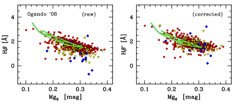
Figure 17: The devised scheme for H$\beta$ correction, as in Fig. 9, is applied to the Ogando et al. (2008) early-type galaxy sample, displayed in the H$\beta$ versus Mg₂ index plane. The strength of H$\beta_{e}$ gas emission is sized up and subtracted according to eq. (34), taking the observed [OIII]’₅₀₀₇ emission as a proxy. To better appreciate the correction effect, we adopted three different galaxy markers for nearly “quiescent” (i.e. [OIII]’${}_{5007}>-1$ Å, or H$\beta_{e}\ga-0.4$ Å, solid dots), “moderately active” ($-2\leq$[OIII]’${}_{5007}\leq-1$ Å, or $-1.5\la$ H$\beta_{e}\la-0.4$ Å, triangles), and “active” (i.e. [OIII]’${}_{5007}<-2$ Å or H$\beta_{e}\la-1.5$ Å, rombs) galaxies. As a guideline, in both panels we also displayed the Buzzoni, Mantegazza, & Gariboldi (1994) synthesis models for a standard Salpeter IMF and [Fe/H] metallicity parameter between $-0.25$ (upper line) and $+0.22$ dex (lower line). “Ladders” across model sequences tick galaxy age for values of 2, 5, 10, and 15 Gyr, with increasing Mg₂. After correction (right panel), galaxy H$\beta$ index is increased, on average, by $0.25\pm 0.20$ Å along the whole sample, making galaxies to appear, on average, about 20-30% younger and 0.2-0.3 dex metal poorer.

Like the [NI] case, hidden emission can subtly plague the nominal diagnostic scheme for other Lick indices. Indeed, the most debated issue, in this regard, deals with a fair correction of H$\beta$ absorption in the spectra of elliptical galaxies. Compared to all the other Lick indices, H$\beta$ (and its weaker Balmer companions, like H$\gamma$ and H$\delta$, see Worthey & Ottaviani, 1997) is the only feature that positively correlates with the effective temperature of stars (see, e.g. Fig. 4 in Trager et al., 1998). As it becomes strongest among A-type stars, this makes the index of special interest to break model degeneracy in the age diagnostic of old- and intermediate- ($t\la 1$ Gyr) age galaxies (Buzzoni, Mantegazza, & Gariboldi, 1994; Worthey, 1994; Maraston & Thomas, 2000; Tantalo & Chiosi, 2004). On the other hand, as gas and stars within a galaxy are conflicting in their line contribution (the first, by emitting, the latter ones by absorbing), the integrated H$\beta$ strength displays the net effect of this interplay.

In Sec. 3.2 we tackled the González (1993) well experienced correction procedure, that relies on the measure of the adjacent [OIII] forbidden emission at 5007 Å, as a proxy to infer the H$\beta$ gaseous contribution. Several physical arguments can be advocated to question such a straightforward relationship between the two emission lines, in consequence of a range of different evolutionary mechanisms (in primis LINER activity) at work. However, one can admittedly assume [OIII] emission to be a generic (but not exclusive) tracer of star-forming activity (and the implied presence of HII gas clouds) within a young stellar population.

Taking a set of spectroscopic observations of 20 bright elliptical galaxies, originally aimed at studying radial spectrophotometric gradients (Carrasco et al., 1995; Buzzoni et al., 2009b, 2015), we devised a simple and robust diagnostic scheme to probe the possible [OIII] versus H$\beta$ entanglement. As observations were taken symmetrically across the galaxy major axis, one can reasonably assume that, whatever the distinctive evolutionary properties, the same stellar population (and, on average, gas content) is sampled at the same radial distance, on opposite sides from the galaxy center. If this is the case, then the H$\beta$ and [OIII]₅₀₀₇ index differences between the two galaxy sides can be contrasted in search for possible statistically correlations. One major advantage of this approach is that it is nominally free from zero-point and other calibration problems with the data, just relying on the assumed central symmetry of the galaxy stellar population.

Our results, summarized in Fig. 8 and Table 3, basically confirm González’ (1993) correction figure of $\Delta H\beta/\Delta[OIII]_{5007}\sim 0.7\pm 0.5$, but only for those ellipticals with established on-going star-formation activity and stronger core emission (i.e. $[OIII]_{5007}\la-1.5$ Å). As far as more quiescent galaxies are considered, any H$\beta$ emission is found to fade out more quickly than [OIII]₅₀₀₇ emission, and this suggests a milder correction scheme, that we parameterized by means of a logistic curve (see Fig. 9), as in eq. (33) and (34).

The effect of our H$\beta$ correction can be appreciated by looking again at the Ogando et al. (2008) sample of elliptical galaxies, as in Fig. 17. The corrected galaxy distribution in the H$\beta$ versus Mg₂ plane is shown in the right panel of the figure, compared with the original sample, as in the left panel. Just as a guideline, the Buzzoni, Mantegazza, & Gariboldi (1994) models are overplotted, throughout. One can notice that most of those galaxies with “shallow” (or negative) H$\beta$ in the left panel are effectively recovered by the procedure, leading eventually to a much cleaner H$\beta$ versus Mg₂ relationship. Along the whole galaxy sample, the corrected H$\beta$ index slightly increases, on average, by $\Delta H\beta\simeq 0.25\pm 0.20$ Å. Although apparently negligible, this figure has important impacts on the inferred galaxy age, which typically shifts toward 20-30% younger values with a 0.2-0.3 dex poorer inferred metallicity (Buzzoni, Mantegazza, & Gariboldi, 1994; Worthey, 1994).

Aside the H$\beta$ problem, the striking importance of the [OIII]₅₀₀₇ forbidden line also emerged along our discussion on Sec. 3.2 when dealing with the intrinsic strength of the Fe5015 index. From one hand, any intervening [OIII]₅₀₀₇ emission will decrease Fe5015 strength as it adds flux to the feature window of the latter. On the other hand, the broader and stronger Fe5015 absorption in the integrated spectrum of old stellar populations may artificially depress the apparent [OIII]₅₀₀₇ luminosity, thus leading to underestimate its equivalent width. In our analysis, we tackled in some detail the problem of a mutual correction of the two indices devising a general procedure that could straightforwardly be applied to other similar contexts, as well. The intrinsic [OIII]₅₀₀₇ strength can therefore be derived in terms of observed quantities, via eq.(31), while the intrinsic Fe5015 index, corrected for O-emission, simply derives from eq. (27).

One important consequence of our analysis is that corrected Fe5015 index is generally expected to increase in the galaxy spectrum, opposite to Mgb trend. This feature may have some impact when combining the two indices, like in the [MgFe50] meta-index, so extensively used for instance in the Sauron studies (Kuntschner et al., 2010; Falcón-Barroso et al., 2011). An intersting comparison can be done, in this regard, with Peletier et al. (2007, see, in particular, Fig. 3, therein). In the plot, when taking the Thomas, Maraston, & Bender (2003) stellar population synthesis models as a reference in the Fe5015 vs. Mgb domain, it appears that Sauron ellipticals better match the $\alpha$-enhanced models with respect to the standard solar chemical partition. On the other hand, one may argue that this is the natural consequence of a relatively “strong” Mgb and “shallow” Fe5015 so that, when accounting for the envisaged corrections, the net effect on the fit is to mitigate any inferred $\alpha$-element enhancement of the galaxy population.

For its relevance, the Mg index complex (including Mgb, Mg₁, and Mg₂ indices) has been the focus of our specific analysis in Sec. 3.3. In its original intention, the Lick system aimed at singling out the atomic and molecular contribution to the broad “Mg valley” about 5150 Å (Faber, Burstein, & Dressler, 1977). This evidently leads to conceive some entanglement among the three indices, that we theoretically assessed, for the first time, by means of eq. (43). This inherent relationship can be usefully relied upon in case of incomplete spectral observations, either to derive the missing index (within a $\sim$1.5% internal accuracy) given the other two or, even more importantly, to assess any possible deviation from the standard scheme, as due to intervening bias effects in the spectra. This has actually been our approach, for instance, to single out the [NI]₅₁₉₉ contribution, as shown in Fig. 13.

As far as low-resolution spectra are dealt with, as in any Lick analysis, we are left with the unescapable consequence that any absorption feature is in fact a blend of a coarse elemental contribution. As we have shown in Sec. 3.5, this problem has been widely explored, from a theoretical point of view, in the recent literature (the work of Serven, Worthey, & Briley, 2005, is probably the most up-to-date attempt in this sense) in order to assess index “responsiveness” to the different chemical species that may potentially intervene at the relevant wavelength of the blended absorption feature. On the other hand, one has to notice in this regard that, for its inherent definition, Lick-index strength directly stems from the residual “in-band” elemental contribution to the feature itself, compensated by the corresponding “off-band” contribution to the flanking pseudo-continuum. Contrary to high-resolution spectroscopy, therefore, a tricky situation may actually set in, where the Lick-index christening element (that is the one with the deepest absorption within the feature window) is not necessarily the representative one that constrains the index strength, as a whole.

As a recognized example (Trager et al., 1998; Serven, Worthey, & Briley, 2005), in Sec. 3.5 we retook in somewhat finer detail the case of Fe4531, one among the many bona fide Iron tracers in the optical spectrum of galaxies, according to the classical Lick scheme. For our analysis we relied on the Sun and Arcturus observed spectra as typical main-sequence and red-giant stellar templates, in an attempt to extend our conclusions also to the old-galaxy framework, according to more elaborated stellar population synthesis models. The comparison of Table 4 and 5 is illuminating to catch the sense of our analysis.

One sees, in fact (Table 4) that, both in the Sun and Arcturus (and, by inference, in the spectrum of elliptical galaxies, for instance), Iron is undoubtedly the leading contributor to the absorption feature at 4531 Å, but once clearing the Fe coarse absorption in the nearby pseudo-continuum as well, it is actually Titanium that, almost solely, commands the game (Table 5) and eventually modulates Fe4531 index behaviour. As a final consideration, the case of Fe4531 and more generally the essence of all our previous discussion, evidently urge an important rethinking process of the Lick-index tool, to bring it fresh life and even better tuned diagnostic performance in view of its updated application to the new-generation spectral data to come.

References

- Bernardi et al. (2006) Bernardi M., Nichol R. C., Sheth R. K., Miller C. J., Brinkmann J., 2006, AJ, 131, 1288
- Bertone et al. (2004) Bertone E., Buzzoni A., Rodríguez-Merino L. H., Chávez M., 2004, MmSAI, 75, 158
- Bertone et al. (2008) Bertone E., Buzzoni A., Chávez M., Rodríguez-Merino L. H., 2008, A&A, 485, 823
- Bettoni & Buson (1987) Bettoni D., Buson L. M., 1987, A&AS, 67, 341
- Beuing et al. (2002) Beuing J., Bender R., Mendes de Oliveira C., Thomas D., Maraston C., 2002, A&A, 395, 431
- Bolzonella et al. (2010) Bolzonella M., et al., 2010, A&A, 524, AA76
- Bressan, Chiosi, & Tantalo (1996) Bressan A., Chiosi C., Tantalo R., 1996, A&A, 311, 425
- Brodie & Huchra (1990) Brodie J. P., Huchra J. P., 1990, ApJ, 362, 503
- Burstein et al. (1984) Burstein D., Faber S. M., Gaskell C. M., Krumm N., 1984, ApJ, 287, 586
- Buzzoni (1995) Buzzoni A., 1995, ApJS, 98, 69
- Buzzoni, Gariboldi, & Mantegazza (1992) Buzzoni A., Gariboldi G., Mantegazza L., 1992, AJ, 103, 1814
- Buzzoni, Mantegazza, & Gariboldi (1994) Buzzoni A., Mantegazza L., Gariboldi G., 1994, AJ, 107, 513
- Buzzoni et al. (2001) Buzzoni A., Chavez M., Malagnini M. L., Morossi C., 2001, PASP, 113, 1365
- Buzzoni et al. (2005) Buzzoni A., Bertone E. Rodríguez-Merino L. H., Chávez M., 2005, in Multiwavelength mapping of galaxy formation and evolution, proc. of the ESO Workshop, ed. A. Renzini and R. Bender (ESO: Garching) p. 361
- Buzzoni, Bertone, & Chavez (2009a) Buzzoni A., Bertone E., Chavez M., 2009, ApJ, 703, L127
- Buzzoni et al. (2009b) Buzzoni A., Battistini C., Carrasco L., Recillas E., 2009b, RMxAC, 37, 110
- Buzzoni et al. (2015) Buzzoni A., Salsa, M., Battistini C., Carrasco L., Recillas E., 2015, ApJ, in preparation
- Caldwell (1984) Caldwell N., 1984, PASP, 96, 287
- Cappellari et al. (2011) Cappellari M., et al., 2011, MNRAS, 413, 813
- Cardiel et al. (1998) Cardiel N., Gorgas J., Cenarro J., Gonzalez J. J., 1998, A&AS, 127, 597
- Carollo, Danziger, & Buson (1993) Carollo C. M., Danziger I. J., Buson L., 1993, MNRAS, 265, 553
- Carson & Nichol (2010) Carson D. P., Nichol R. C., 2010, MNRAS, 408, 213
- Clemens et al. (2006) Clemens M. S., Bressan A., Nikolic B., Alexander P., Annibali F., Rampazzo R., 2006, MNRAS, 370, 702
- Crocker et al. (2011) Crocker A. F., Bureau M., Young L. M., Combes F., 2011, MNRAS, 410, 1197
- Carrasco et al. (1995) Carrasco L., Buzzoni A., Salsa M., Recillas-Cruz E., 1995, ASPC, 86, 235
- Coelho et al. (2005) Coelho P., Barbuy B., Meléndez J., Schiavon R. P., Castilho B. V., 2005, A&A, 443, 735
- Colless et al. (1999) Colless M., Burstein D., Davies R. L., McMahan R. K., Saglia R. P., Wegner G., 1999, MNRAS, 303, 813
- Conroy (2013) Conroy C., 2013, ARA&A, 51, 393
- Davies et al. (1987) Davies R. L., Burstein D., Dressler A., Faber S. M., Lynden-Bell D., Terlevich R. J., Wegner G., 1987, ApJS, 64, 581
- de Vaucouleurs et al. (1991) de Vaucouleurs, G., de Vaucouleurs, A., Corwin, H.G. Jr., Buta, R.J., Paturel, G., Fouque, P. 1991, Third Reference Catalog of Bright Galaxies. Springer Verlag, Heidelberg
- Dobos et al. (2012) Dobos L., Csabai I., Yip C.-W., Budavári T., Wild V., Szalay A. S., 2012, MNRAS, 420, 1217
- Domínguez Sánchez et al. (2011) Domínguez Sánchez H., et al., 2011, MNRAS, 417, 900
- Faber (1973) Faber S. M., 1973, A&AS, 10, 201
- Faber & Jackson (1976) Faber S. M., Jackson R. E., 1976, ApJ, 204, 668
- Faber, Burstein, & Dressler (1977) Faber S. M., Burstein D., Dressler A., 1977, AJ, 82, 941
- Faber et al. (1985) Faber S. M., Friel E. D., Burstein D., Gaskell C. M., 1985, ApJS, 57, 711
- Falcón-Barroso et al. (2011) Falcón-Barroso J., et al., 2011, MNRAS, 417, 1787
- Ferland et al. (2012) Ferland G. J., Henney W. J., O’Dell C. R., Porter R. L., van Hoof P. A. M., Williams R. J. R., 2012, ApJ, 757, 79
- Fritze-v. Alvensleben (1998) Fritze-v. Alvensleben U., 1998, HiA, 11, 78
- Fusi Pecci et al. (2005) Fusi Pecci F., Bellazzini M., Buzzoni A., De Simone E., Federici L., Galleti S., 2005, AJ, 130, 554
- Geary (1930) Geary R. C., 1930, Journal of the Royal Stat. Soc., 93, 442
- Golay (1974) Golay M., 1974, Introduction to Astronomical Photometry, Astroph. & Sp. Sc. Lib., Vol. 41, (Reidel, Dordrecht)
- González (1993) González J. J., 1993, PhD Thesis, Univ. of Santa Cruz
- González et al. (2012) González V., Bouwens R. J., Labbé I., Illingworth G., Oesch P., Franx M., Magee D., 2012, ApJ, 755, 148
- Gorgas, Efstathiou, & Aragon Salamanca (1990) Gorgas J., Efstathiou G., Aragon Salamanca A., 1990, MNRAS, 245, 217
- Gorgas et al. (1993) Gorgas J., Faber S. M., Burstein D., Gonzalez J. J., Courteau S., Prosser C., 1993, ApJS, 86, 153