Order and disorder in irreversible decay processes

Abstract

Dynamical disorder motivates fluctuating rate coefficients in phenomenological, mass-action rate equations. The reaction order in these rate equations is the fixed exponent controlling the dependence of the rate on the number of species. Here we clarify the relationship between these notions of (dis)order in irreversible decay, $n\,A\to B$, $n=1,2,3,\ldots$, by extending a theoretical measure of fluctuations in the rate coefficient. The measure, $\mathcal{J}_{n}-\mathcal{L}_{n}^{2}\geq 0$, is the magnitude of the inequality between $\mathcal{J}_{n}$, the time-integrated square of the rate coefficient multiplied by the time interval of interest, and $\mathcal{L}_{n}^{2}$, the square of the time-integrated rate coefficient. Applying the inequality to empirical models for non-exponential relaxation, we demonstrate that it quantifies the cumulative deviation in a rate coefficient from a constant, and so the degree of dynamical disorder. The equality is a bound satisfied by traditional kinetics where a single rate constant is sufficient. For these models, we show how increasing the reaction order can increase or decrease dynamical disorder and how, in either case, the inequality $\mathcal{J}_{n}-\mathcal{L}_{n}^{2}\geq 0$ can indicate the ability to deduce the reaction order in dynamically disordered kinetics.

I Introduction

Observing the natural world, one constant seems to be that systems have the capacity for chemical and physical change, though the mechanisms for change vary. Measuring rates of change is a common approach for deducing the mechanism of kinetic processes. Complex chemical reactions are an example where the rate equation governing molecular transformations can be evidence of a particular mechanism. Houston (2006) For this reason, chemical kinetics provides a set of methods to quantify the parameters of the rate equation: the rate coefficient and the order(s). Steinfeld, Francisco, and Hase (1989) These empirical parameters define the dynamical equations, which are the typical mass-action rate equations, provided the reaction system is homogeneous – as in a solution phase chemical reaction under standard conditions with uniform concentration(s) throughout. Rate processes with “disorder”, however, deviate from traditional rate equations. Ross (2008) In disordered rate processes, Zwanzig (1990) it is necessary to replace the rate constant in the rate equation with an effective time-dependent rate coefficient. The origin of this deviation from classical kinetics is often microscopic structural and energetic changes in the host environment, which occur on a time scale comparable to the chemical change. Plonka (2001)

An early example of disordered or dispersed kinetics is the rebinding of carbon monoxide to hemeproteins following photodissociation. Austin et al. (1975) Experiments showed the complexity of this process is due to a multitude of energy barriers and reaction pathways. More recent advances in single-molecule techniques are bringing attention to the disordered decay Chakrabarti and Bagchi (2003) of structural correlations in biomolecules during electron transfer reactions Luo et al. (2006) and enzyme catalyzed reactions. Terentyeva et al. (2012); English et al. (2005); Min et al. (2005); Flomenbom et al. (2005) Experimental techniques have also inspired new theoretical approaches to disordered kinetics Wang and Wolynes (1994, 1993, 1995) in the forced unfolding Kuo et al. (2010); Chatterjee and Cherayil (2011) and spontaneous folding Lee, Stell, and Wang (2003); Zhou et al. (2003) of biomolecules. Disordered kinetics is also of interest in the charge transfer through molecular assemblies because of their potential use in molecular electronics, solar cells, and artificial photosynthesis. Berlin et al. (2008); *GrozemaBSR10 These diverse applications motivate the search for organizing principles and theoretical frameworks for extracting mechanistic information that extend chemical kinetics. The present work develops such a framework.

In the examples above, “disorder” can be the result of an intrinsically time-dependent reaction environment (pure dynamical disorder, homogeneous), a spatially-dependent reaction environment with an underlying, unknown distribution of rate coefficients (static disorder, heterogeneous), or both. In any case, the overall kinetics is describable by a single time-dependent rate coefficient, with underlying rate coefficients that can fluctuate in time or space. The reaction order of the overall kinetics, however, is a constant; as in traditional kinetics, the reaction “order” in the rate equation is the power of the concentration dependence of the rate. While the reaction order can be evidence of a particular mechanism in traditional kinetics, it is not clear whether the reaction order might provide mechanistic clues in kinetics with dynamical disorder. As a step in this direction, our interest here is in the temporal variation of an effective, overall rate coefficient for disordered kinetic processes, and how this disorder relates to reaction order.

Relaxation or irreversible decay phenomena have been the primary focus of theoretical and computational works in disordered kinetics. Ross (2008) There has been a particular theoretical emphasis on first-order decay Zwanzig (1990); however, under some circumstances, disordered processes can have higher-order rate equations; for example, this was shown for a case of dispersive, early stage protein folding kinetics. Metzler et al. (1998); Plonka (2000) Complicating the mechanistic insights that can come from rates, is that experimental data may agree with both first- and second-order rate equations when the rate coefficient is time dependent. A further complication is that multiple microscopic models can lead to the same macroscopic relaxation behavior; an example for first-order decay are the mechanisms consistent with the stretched-(non)-exponential decay. Klafter and Shlesinger (1986) These findings stimulate our investigation into how meaningful the traditional notion of reaction-order is for phenomenological, non-exponential kinetic data.

Here we consider the dynamic disorder in the macroscopic kinetics of the irreversible processes

$$n\,A\to B\quad\quad\textrm{for}\quad n=1,2,3,\ldots.$$ (1)

We assume the concentration, $C_{n}(t)$, of the species $A$ obey the (non-)linear differential rate equations

$$\frac{dC_{n}(t)}{dt}=-k_{n}(t)\left[C_{n}(t)\right]^{n}$$ (2)

with time-dependent, effective rate coefficients $k_{n}(t)$. That is, the rates are $n^{\textrm{th}}$-order in $A$. [The subscript $n$ will distinguish variables and parameters of rate processes of different reaction order.] Since these rate equations are solvable for any $n$, we will consider the entire class of reactions. However, the highest known order of a chemical reaction is third order in traditional kinetics, $k(t)\to k$. Steinfeld, Francisco, and Hase (1989) In disordered kinetics, second-order seems to be the highest known order in agreement with experimental results. For example, power law decays describing recombination reactions and peptide folding satisfy second-order rate equations, Plonka, Kroh, and Berlin (1988); Plonka, Berlin, and Chekunaev (1989); Hamill (1981) though stretched exponential functions also fit the available data. Metzler et al. (1998); Plonka (2000) Generalized functions, encompassing both stretched exponential and power law decay are also known. Brouers and Sotolongo-Costa (2006)

II Theoretical background

Static and dynamic disorder lead to an observed rate coefficient, $k_{n}(t)$, that depends on time in macroscopic rate equations. The time dependence can stem from fluctuations in the rate coefficient, fluctuations due to the heterogeneity of the system and/or the reaction environments. Measuring the dispersion of the rate coefficients is therefore a natural approach to quantify the involvement of the environment in the mechanism or the structural disorder of the medium. Dewey (1992) The degree of variation in the observed rate coefficient also quantifies the fidelity of a rate coefficient or rate equation, assuming rate coefficients that vary less over the observational time scale are more desirable.

A cumulative measure of disorder that we extend here, originally in Reference Flynn, Zhao, and Green, 2014, is the magnitude of the inequality

$$\mathcal{J}_{n}(\Delta{t})\geq\mathcal{L}_{n}(\Delta{t})^{2}$$ (3)

between the statistical length (squared)

$$\mathcal{L}_{n}(\Delta{t})^{2}\equiv\left[\int_{t_{i}}^{t_{f}}k_{n}(t)dt\right]^{2}$$ (4)

and the divergence

$$\mathcal{J}_{n}(\Delta{t})\equiv\Delta{t}\int_{t_{i}}^{t_{f}}k_{n}(t)^{2}dt$$ (5)

over a time interval $\Delta t=t_{f}-t_{i}$. From these definitions, $\mathcal{L}_{n}$ and $\mathcal{J}_{n}$ are functions of a possibly time-dependent rate coefficient. The statistical length, $\mathcal{L}_{n}$, we use is the cumulative time-dependent rate coefficient over a period of time $\Delta{t}$, and the divergence, $\mathcal{J}_{n}$, is the cumulative square of the rate coefficient, multiplied by the time interval. These definitions are independent of the particular system and could be applied to any disordered kinetic process with a time-dependent rate coefficient. The difference, $\mathcal{J}_{n}-\mathcal{L}_{n}^{2}$, quantifies both the variation of $k_{n}(t)$ in time and the fraction of the observation time where those changes occur. As a measure of disorder, the inequality is complementary to other information theoretic measures of dynamic disorder. Li and Komatsuzaki (2013); Chekmarev (2008)

The representation of $\mathcal{J}_{n}$ and $\mathcal{L}_{n}$ we define above is just one from our earlier work on first-order ($n=1$) rate processes, Flynn, Zhao, and Green (2014) which established a connection between the rate coefficient and a modified Fisher information. Frieden (2004) For first-order rate processes, the inequality above has two important features: (1) $\mathcal{J}_{1}-\mathcal{L}^{2}_{1}$ measures the variation of the rate coefficient in statically or dynamically disordered decay kinetics over a time interval of interest, and (2) the lower bound, $\mathcal{J}_{1}=\mathcal{L}^{2}_{1}$, holds only when the effective rate coefficient is constant. These features are sensitive to the definition of the time-dependent rate coefficient, $k_{n}(t)$, but we will show that defining it appropriately, the inequality applies to irreversible decay kinetics with non-linear rate laws (i.e., kinetics with total reaction-order greater than unity). We illustrate this framework with proof-of-principle models for irreversible decay phenomena of total reaction-order greater than one.

In macroscopic chemical kinetics, experimental data are typically a concentration profile corresponding to the integrated rate equation. For a population of species irreversibly decaying over time, we define the survival function for $n^{\textrm{th}}$-order decay,

$$S_{n}(t)=\frac{C_{n}(t)}{C_{n}(0)}.$$ (6)

For truly irreversible decay, this is the probability the initial population survives up to a time $t$. In traditional first-order kinetics the survival probability, $e^{-\omega_{1}t}$, is characterized by a rate constant $\omega_{1}$. Linear fitting methods of survival data are a standard approach to find an empirical rate equation. For example, for a first-order process, a plot of $\ln S_{1}(t)$ versus time $t$ is linear with a slope of $-\omega_{1}$ only if the traditional first-order rate equation is valid. If the graph is non-linear, it is natural to search for a higher-order rate equation that gives a linear graph. Houston (2006) Another approach is to introduce a time-dependent rate coefficient $k_{1}(t)$ describing the non-exponential decay, when one suspects members of the population decay in different structural or energetic environments or in a local environment that fluctuates in time. This approach should extend to higher reaction orders, but seems to have received less attention than the case of first-order kinetics.

We define the effective rate coefficient, $k_{n}(t)$, through an appropriate time derivative of the survival function, depending on the reaction-order, $n$,

$$k_{n}(t)\equiv\begin{cases}\displaystyle-\frac{d}{dt}\ln S_{1}(t)&\text{if }n=1\\[10.0pt] \displaystyle+\frac{1}{n-1}\frac{d}{dt}\frac{1}{S_{n}(t)^{n-1}}&\text{if }n\geq 2.\end{cases}$$ (7)

In any case, $k_{n}(t)$ has dimensions of inverse time. The survival function is dimensionless, which prevents $k_{1}(t)$ from having a logarithmic argument with units. While the survival function is not necessary on the grounds of units for $n\geq 2$, we use it to keep the interpretation of $S(t)$ as a survival probability and to maintain consistency with our previous work. Flynn, Zhao, and Green (2014)

With these $k_{n}(t)$, we can express the statistical length, $\mathcal{L}_{n}$, and the divergence, $\mathcal{J}_{n}$, for any reaction order. It is then straightforward to show these $k_{n}(t)$, give the bound $\mathcal{J}_{n}=\mathcal{L}_{n}^{2}$ if $k_{n}(t)$ is independent of time. As an example, consider an $n^{th}$-order reaction where $n\geq 2$. The traditional integrated rate equation is the time dependence of the concentration, $C_{n}(t)$,

$$\frac{1}{C_{n}(t)^{n-1}}=\frac{1}{C_{n}(0)^{n-1}}+(n-1)\omega_{n}t.$$ (8)

When $n\neq 1$, the rate constant, $\omega_{n}$, has dimensions of [time]^-1 $\cdot$ [concentration]^-(n-1). From the general definition in Equation 6, the survival function is

$$S_{n}(t)=\sqrt[n-1]{\frac{1}{1+(n-1)\omega_{n}C_{n}(0)^{n-1}t}}$$ (9)

and the definition of the effective rate coefficient is $k_{n}(t)\to\omega_{n}C_{n}(0)^{n-1}$. This time-independent rate coefficient gives $\left[\omega_{n}\Delta tC_{n}(0)^{n-1}\right]^{2}$ for both the statistical length squared and the divergence. That is, the bound $\mathcal{J}_{n}=\mathcal{L}_{n}^{2}$ holds when there is no static or dynamic disorder, and a single rate coefficient, $\omega_{n}$, is sufficient to characterize irreversible decay. When the kinetics are statically or dynamically disordered, the rate coefficient governing irreversible decay is not constant and one must work with the above definitions of $k_{n}(t)$.

III Results and discussion

III.1 Kinetic model with disorder

To study the effect of dynamical disorder on kinetics with reaction orders greater than one, we adapt the Kohlrausch-Williams-Watts (KWW) model. Kohlrausch (1854); Williams and Watts (1970); Plonka (2001) The procedure is similar to that of first-order kinetics where exponential decay is “stretched” to characterize non-exponential decays with a two-parameter survival function $\exp[-(\omega_{1}t)^{\beta}]$. The parameter $\omega_{1}$ is a characteristic rate constant or inverse time scale and the parameter $\beta$ is a measure of the degree of stretching; both parameters depend on the system and can depend on external variables such as temperature and pressure. Plonka (2001) This procedure for modifying traditional kinetics introduces a time-dependent rate coefficient, $k_{1,\beta}(t)=\beta(\omega_{1}t)^{\beta}/t$, into the empirical model. While different mechanisms can lead to stretched exponential decay, Klafter and Shlesinger (1986) and any model with a time-dependent rate coefficient can be subject to our analysis, this type of decay is a good example for our purposes, given its generality. Brouers and Sotolongo-Costa (2006)

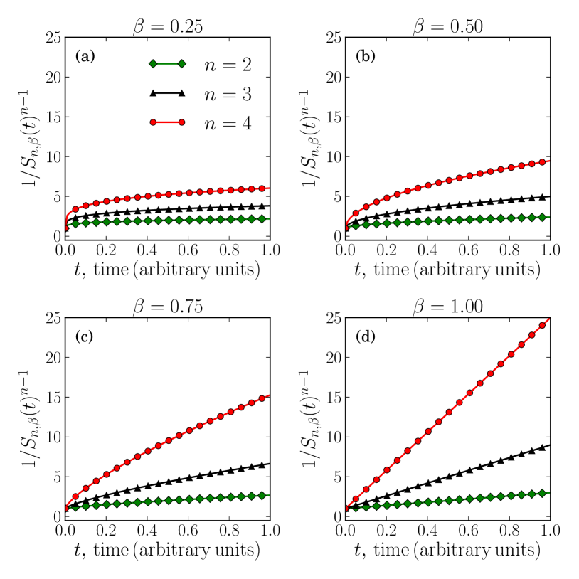
Figure 1: When the disorder parameter, $\beta$, is (a) $0.25$, (b) $0.50$, or (c) $0.75$ the function $1/S_{n,\beta}^{n-1}(t)$ is non-linear in time. This non-linearity motivates the use of an effective time-dependent rate coefficient for the overall decay when the rate equation is known to be $n^{\textrm{th}}$-order in the decaying population. Traditional $n^{\textrm{th}}$-order kinetics corresponds to the special case of (d) $\beta=1$, where the rate coefficient is time independent and comes from the slope of these plots, $\omega_{n}C_{n}(0)^{n-1}$. Here $C_{n}(0)=2$ and $\omega_{n}=1$ in arbitrary units. The effective, time-dependent rate coefficient is proportional to the slope at a given time.

We introduce disorder and a time-dependent rate coefficient into “higher-order” kinetics through the $n^{\textrm{th}}$-order survival function

$$S_{n,\beta}(t)=\sqrt[n-1]{\frac{1}{1+(n-1)\left[\omega_{n}C_{n}(0)^{n-1}t\right]^{\beta}}}.$$ (10)

Again there is a characteristic rate constant $\omega_{n}$ and disorder parameter $0<\beta\leq 1$. We chose $\omega_{n}=1$ and a fixed observational time scale to simplify the presentation of our results. Plonka and coworkers interpret the stretching parameter for $n=2$, as the result of a time-dependent energy barrier height, and as the result of a superposition of second-order decays. Plonka, Berlin, and Chekunaev (1989) For $n\geq 2$, the characteristic kinetic plot – a graph of $1/S_{n,\beta}^{n-1}$ versus $t$ – is shown in Figure 1. As these graphs illustrate, decreasing the parameter $\beta$ stretches the survival plot for $n^{\textrm{th}}$-order kinetics, just as it does for first-order processes. Another similarity with first-order kinetics is that the limit $\beta=1$ corresponds to traditional kinetics, the absence of disorder, and when the effective rate coefficient, $k_{n}(t)\to\omega_{n}C_{n}(0)^{n-1}$, corresponds to the constant slope of the graph.

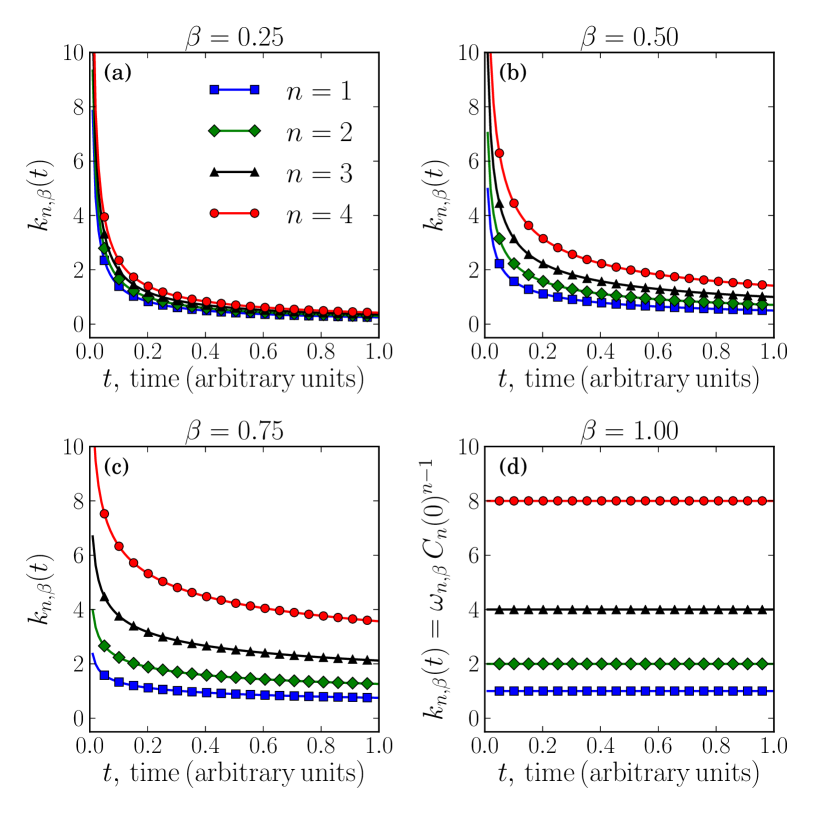
Figure 2: Time-dependence of the effective rate coefficient $k_{n,\beta}(t)$ for varying reaction orders $n=1$, $2$, $3$, and $4$ when $\beta$ is (a) $0.25$, (b) $0.50$, (c) $0.75$, and (d) $1.00$. The $k_{n,\beta}(t)$ of different order $n$ become the same function of time as $\beta\to 0$ and time independent as $\beta\to 1$. In all cases the initial concentration is $C_{n}(0)=2.0$ and the rate constant is $\omega_{n}=1$ in arbitrary units.

At and away from the limit $\beta=1$, the survival functions satisfy rate equations

$$\frac{dS_{n,\beta}(t)}{dt}=-k_{n,\beta}(t)S_{n,\beta}(t)^{n}$$ (11)

with the same form as Equation 2. The effective rate coefficients in these cases are

$$k_{n,\beta}(t) = \beta\left[\omega_{n}C_{n}(0)^{n-1}t\right]^{\beta}/t$$ (12)

$$= C_{n}(0)^{\beta\left(n-1\right)}k_{1,\beta}(t).$$

This definition of the time-dependent rate coefficients differs from that of other authors Metzler et al. (1998) to satisfy the rate equations above. Keep in mind, we define the effective rate coefficient in terms of the dimensionless survival function $S_{n,\beta}(t)$. If we instead define the effective rate coefficient in terms of the concentration, $C_{n,\beta}(t)$, then the effective rate coefficient becomes a constant as $\beta\to 1$, with dimensions of [concentration]^-(n-1) $\cdot$ [time]^-1. We will use the former definition of the effective rate coefficient because the subsequent results will depend on the initial concentration of the decaying species, which is consistent with other results in traditional kinetics (e.g., the half-life depends on the initial concentration in kinetics with $n\geq 2$). Houston (2006)

III.2 Inequality for disorder in irreversible kinetics

Having laid out the details and main aspects of the model, we turn to the application of the theory. For this class of disordered kinetics, it can be difficult to distinguish the survival curves for different $n$ when $\beta$ is small. For example, experimental $\beta$ values around $0.1$ are necessary to fit peptide folding data to a stretched exponential. Metzler et al. (1998); Plonka (2000) In this case, the data are also well fit by an asymptotic power law decay (the integrated form of a second-order rate equation). Our results support this fact, and show it is also true of irreversible decay for higher $n$. Figure 2, shows the time dependence of $k_{n,\beta}(t)$ for $n=1$, $2$, $3$, and $4$ when $\beta$ is (a) $0.25$, (b) $0.50$, (c) $0.75$, and (d) $1.00$. These data are for an initial concentration of $C_{n}(0)=2.0$ and $\omega_{n}=1.0$ in arbitrary units. As $\beta\to 0$ the effective rate coefficient $k_{n,\beta}(t)\to k_{\beta}(t)$, and the corresponding survival plots of all reaction order converge, $S_{n,\beta}(t)\to S_{\beta}(t)$. That is, it can become difficult to distinguish the order of a reaction when $\beta$ is small, which can be taken to mean decay events are highly cooperative or correlated.

When a $\beta$ approaching zero is necessary to fit the available survival data, processes with an order $n\geq 2$ may not be distinguishable from first-order processes. That is, for this widespread type of kinetics, higher-order kinetics may be an equally valid description of experimental data when $\beta$ is small, unless the modeller has more information about the underlying mechanism to suggest a particular reaction order. The greater the value of $\beta$ is, than say $0.1$, the easier it should be to discern rate equations with $n\geq 2$ within the experimental uncertainty. Exactly how small $\beta$ must be for the reaction order to lose meaning will depend on the value of $\omega_{n}$, which we take to be unity, and the observational time scale. When the rate equations of different orders are distinguishable, we will show there is an interesting interplay between order, $n$, and the disorder parameter, $\beta$, that we can disentangle with the measure of dynamical disorder, $\mathcal{J}_{n,\beta}-\mathcal{L}_{n,\beta}$. To do this, we will need the length and divergence.

From the effective rate coefficient for $n\geq 2$, the statistical length is

$$\mathcal{L}_{n,\beta}(\Delta{t})=\left[\omega_{n}C_{n}(0)^{n-1}t\right]^{\beta}\big{|}_{t_{i}}^{t_{f}}$$ (13)

and the divergence is

$$\frac{\mathcal{J}_{n,\beta}(\Delta{t})}{\Delta t}=\beta^{2}\left[\omega_{n}C_{n}(0)^{n-1}\right]^{2\beta}\\ \times\begin{cases}\displaystyle\frac{t^{2\beta-1}}{2\beta-1}\bigg{|}_{t_{i}}^{t_{f}}&\text{if }\beta\neq\tfrac{1}{2}\\[10.0pt] \displaystyle\ln t\big{|}_{t_{i}}^{t_{f}}&\text{if }\beta=\tfrac{1}{2}.\end{cases}$$ (14)

The effective, time-dependent rate coefficient depends on the initial concentration, which carries through to $\mathcal{J}_{n,\beta}$ and $\mathcal{L}_{n,\beta}$. Comparing the inequality for first-order kinetics Flynn, Zhao, and Green (2014) to that of higher-order kinetics, we see the inequalities are related:

$$\mathcal{J}_{n,\beta}-\mathcal{L}_{n,\beta}^{2}=C_{n}(0)^{2\beta\left(n-1\right)}\left[\mathcal{J}_{1,\beta}-\mathcal{L}_{1,\beta}^{2}\right].$$ (15)

The initial concentration, and its dependence upon $n$ and $\beta$, distinguishes the inequality of higher-order kinetics from first-order kinetics. We will examine this relation as a means of determining the reaction order, $n$, in disordered kinetics after exploring the effect of $n$ and $\beta$ on the inequality.

III.3 Disorder and the parameters $\bm{\beta}$ and $\bm{n}$

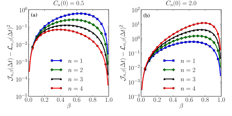
Figure 3: The magnitude of the inequality, $\mathcal{J}_{n,\beta}-\mathcal{L}^{2}_{n,\beta}$, on a logarithmic scale over the range of the disorder parameter, $\beta$, when the initial concentration $C_{n}(0)$ is (a) $0.5$ and (b) $2.0$. Here $\omega_{n}=1$, $t_{i}=1$, and $t_{f}=10$ in arbitrary, but consistent, units. Increasing the reaction order, $n$, can increase or decrease the dynamical disorder, as measured by the inequality, depending on the initial concentration. The inequality correctly reflects the absence of dynamical disorder in the limits $\beta\to 0$ and $\beta=1$.

From these results we can show $\mathcal{J}_{n,\beta}-\mathcal{L}_{n,\beta}^{2}$ measures dynamical disorder for irreversible decay kinetics with $n\geq 1$. A minimum criterion a reasonable measure of disorder must have is that it be zero in the absence of disorder. For the present model, this means the measure must then be zero when $\beta=1$ and tend to zero as $\beta\to 0$, since the rate coefficient $k_{n,\beta}(t)$ is time independent in these limits. Indeed, we find the inequality satisfies this requirement, and the lower bound $\mathcal{J}_{n,\beta}-\mathcal{L}_{n,\beta}^{2}=0$ holds when $\beta=0$, $1$ irrespective of the reaction-order, $n$. It is important to note that this is true when $k_{n}(t)$ is defined as in Equation 12.

Away from the limits $\beta=0$ and $1$, we find the statistical length and divergence are not equal, $\mathcal{J}_{n,\beta}-\mathcal{L}_{n,\beta}^{2}\geq 0$ (Figure 3). Interestingly, for all $n$, their difference initially increases with decreasing $\beta$ from one to zero, since this stretches the survival plot and increases the variation in the effective rate coefficient over the observational time window. However, as $\beta$ decreases further, there is eventually a point at which the rate coefficient is effectively constant over the majority of the observational time window. This leads to an eventual decrease in disorder when stretching $n^{\textrm{th}}$-order kinetics due to the separation of decay into “fast” and “slow” components. The inequality accurately reflects this effect and, consequently, has a maximum in its dependence upon $\beta$, tending to the lower bound $\mathcal{J}_{n,\beta}-\mathcal{L}_{n,\beta}^{2}=0$ as $\beta\to 0$. Another interpretation of the inequality is as a measure of the deviations of the $n^{\textrm{th}}$-order characteristic kinetic plot from linear during observational time window, and the portion of the time window when those deviations occur. The maximum in the inequality results from the competition of these factors. These findings are evidence that the inequality measures the amount of dynamical disorder in irreversible decay processes of any reaction-order.

Figure 3 shows the dependence of the degree of dynamical disorder on the disorder parameter, $\beta$. The inequality reveals a main feature of dynamical disorder: the disorder parameter, $\beta$ does not linearly increase the amount of dynamical disorder in irreversible relaxations describable by stretched exponential and power law ($n\geq 2$, Equation 10) decay. Further, the amount of dynamical disorder measured by the inequality does not uniquely determine the value of $\beta$. Increasing (for $\beta$ values greater than that corresponding to the maximum in $\mathcal{J}_{n,\beta}-\mathcal{L}^{2}_{n,\beta}$) or decreasing $\beta$ (for $\beta$ values less than that corresponding to the maximum in $\mathcal{J}_{n,\beta}-\mathcal{L}^{2}_{n,\beta}$) can improve the approximation of the decay over the observational time scale with a single rate coefficient. We take this as further evidence that the inequality is a useful measure of dynamical disorder.

Comparing panel (a) and (b) in Figure 3, we see the initial concentration dictates whether increasing the reaction-order increases or decreases the inequality, and so, the dynamical disorder for a given $\beta$, $\omega_{n}$, and observational time scale. Panel (a) shows that for an initial concentration $C_{n}(0)<1$, $\mathcal{J}_{n,\beta}-\mathcal{L}_{n,\beta}^{2}$ decreases with reaction order, $n$, at a given $\beta\neq 0$ or $1$. This suggests that for a given $\beta$, higher-order the kinetics will have an effective rate coefficient $k_{n,\beta}(t)$ that varies less over the observational time scale: there is less dynamical disorder with increasing reaction order. In contrast, panel (b) shows the converse is true when the initial concentration $C_{n}(0)>1$: $\mathcal{J}_{n,\beta}-\mathcal{L}_{n,\beta}^{2}$ increases with reaction order, $n$, suggesting $k_{n,\beta}(t)$ varies more over the observational time scale the higher-order the kinetics. Overall, higher reaction-order processes can have more or less disorder for a given ($\beta$, $\omega_{n}$, $\Delta t$) depending on the initial concentration. The reaction-order is not the opposite of dynamical disorder.

Among the growing number of disordered systems, Plonka (2001); Ross (2008) a couple of interesting applications of our approach would be peptide folding Metzler et al. (1998) and low-temperature recombination reactions, such as the recombination of carbon monoxide with myoglobin, Austin et al. (1975) which have small stretching parameters ($\beta\approx 0.1$). Inspecting Figure 3 around $\beta=0.1$ we find there are $n$-dependent differences in the $\mathcal{J}_{n,\beta}-\mathcal{L}_{n,\beta}^{2}$ curves. At $\beta=0.1$ the inequality is small and only weakly dependent on the reaction order. This is quantitative evidence of why experimental peptide folding data that is well fit by a stretched exponential ($n=1$) with a $\beta$ value around $0.1$ is also fit by an asymptotic power law decay ($n=2$). The near equivalence of $\mathcal{J}_{1,\beta}-\mathcal{L}^{2}_{1,\beta}$ and $\mathcal{J}_{2,\beta}-\mathcal{L}^{2}_{2,\beta}$ for reactions of different $n$ suggests the degree of disorder is approximately the same within experimental uncertainties. This result also suggests higher-reaction-orders may fit this data.

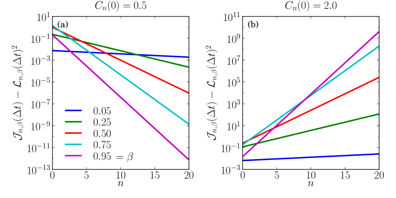
Figure 4: The magnitude of the inequality, $\mathcal{J}_{n,\beta}-\mathcal{L}^{2}_{n,\beta}$, on a logarithmic scale over the range of the reaction-order, $n$, when the initial concentration $C_{n}(0)$ is (a) $0.5$ and (b) $2.0$. Here $\omega_{n}=1$, $t_{i}=1$, and $t_{f}=10$ in arbitrary, but consistent, units. The disorder parameter, $\beta$, controls how strongly the dynamical disorder, as measured by the inequality, depends on the reaction-order, $n$, regardless of the initial concentration. When $\beta=1$, $\mathcal{J}_{n,\beta}=\mathcal{L}^{2}_{n,\beta}$ for all $n$.

Using this model for irreversible decay, we can also consider the dependence of the inequality on the reaction-order parameter, $n$. Figure 4 shows that $\beta$ determines how strongly the inequality (dynamical disorder) depends on the reaction order. We see increasing $\beta$ strengthens the dependence of the dynamical disorder on the reaction-order – whether the dynamical disorder increases or decreases with $n$. In particular, as $\beta\to 0$ the degree of dynamical disorder, as measured by the inequality, becomes more uniform over the range of $n$; the dynamical disorder becomes independent of the reaction order. Furthermore, this finding is independent of the initial concentration, as the two panels show. We also saw that as $\beta\to 0$, the $n$-dependent variations in the effective rate coefficient vanish, $k_{n,\beta}(t)\to 0$ in Figure 2, which is why $\mathcal{J}_{n,\beta}-\mathcal{L}_{n,\beta}^{2}$ also becomes independent of $n$. Since the parameter $\beta$ determines the rate of change of $\mathcal{J}_{n,\beta}-\mathcal{L}_{n,\beta}^{2}$ with $n$, for small $\beta$, the lack of variation of the inequality with $n$ suggests a fundamental difficulty in determining the reaction order. These results are another reflection of the difficulty in determining the reaction order in non-exponential kinetics when $\beta$ is small.

III.4 Disorder and the initial concentration, $\bm{C_{n}(0)}$

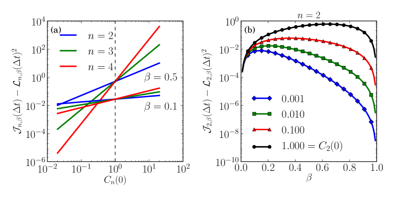
Figure 5: (a) A log-log plot of the inequality, $\mathcal{J}_{n,\beta}-\mathcal{L}^{2}_{n,\beta}$, as a function of the initial concentration, $C_{n}(0)$, for $n=2-4$ and $\beta=0.1$, $0.5$. (b) The inequality, $\mathcal{J}_{2,\beta}-\mathcal{L}^{2}_{2,\beta}$, for second-order kinetics on a log scale versus the disorder parameter, $\beta$, for initial concentrations, $C_{n}(0)$, spanning four orders of magnitude and a fixed observational time scale ($t_{i}=1$, $t_{f}=10$).

In traditional macroscopic kinetics, initial rate methods are a standard means of determining the order(s) in the rate equation. Initial rate methods involve varying the initial concentration of a particular reactant, and measuring the initial rate. Through a series of such measurements, an experimenter can find the order of a hypothesized rate equation through algebraic manipulation, and gain clues about the mechanism of the reaction. We take a similar approach for the present model of disordered kinetics. Figure 5(a) shows a log-log plot of $\mathcal{J}_{n,\beta}-\mathcal{L}^{2}_{n,\beta}$ as a function of the initial concentration, $C_{n}(0)$, for $n=2-4$ and $\beta=0.1$, $0.5$. The inequality is over the observational time window, $t_{i}=1$ and $t_{f}=10$.

Most immediate from these data is that the magnitude of the inequality, and the dynamical disorder it represents, directly correlates with $C_{n}(0)$ for all $\beta$ and $n$. At a given $\beta$, $\mathcal{J}_{n,\beta}-\mathcal{L}_{n,\beta}^{2}$ may increase or decrease with reaction-order, $n$, depending on the initial concentration: the inequality increases with $n$ for $C_{n}(0)>1$ and decreases for $C_{n}(0)<1$, as shown in Figures 3 and 4. Also of note is that while $\mathcal{J}_{n,\beta}-\mathcal{L}_{n,\beta}^{2}$ increases more rapidly for $n=4$ than $n=2$, the difference can be offset by a small $\beta$, e.g., $0.1$. This detail reflects the more general finding that the “strength” of the increase or decrease of the inequality depends on $\beta$; decreasing the value of $\beta$ suppresses the concentration dependence of the dynamical disorder (inequality) for all reaction orders, and the differences in the inequality for different $n$. Thus, even the initial concentration dependence may not be sufficient to distinguish the disordered kinetics of reactions with different reaction order.

Figure 5(b), shows how the inequality for second-order kinetics, $\mathcal{J}_{2,\beta}-\mathcal{L}^{2}_{2,\beta}$, varies with the disorder parameter, $\beta$, for initial concentrations, $\omega_{n}C_{n}(0)$, spanning four orders of magnitude and a fixed observational time scale. The maximum in the inequality at $\beta_{\textrm{max}}$ shifts to larger $\beta$ values with increasing $C_{2}(0)$. Similar behavior results from increasing $\omega_{2}$, which we have set to one. For $\beta<\beta_{\textrm{max}}$, $\beta$ and $n$ have the opposite effect on the dynamical disorder: increasing $\beta$ and decreasing $n$ will increase the dynamical disorder. But if $\beta>\beta_{\textrm{max}}$, $\beta$ and $n$ have the same effect on the dynamical disorder: decreasing $\beta$ and decreasing $n$ will increase the dynamical disorder. We conclude that $n$ and $\beta$ are not strictly opposed parameters of order and disorder, and the inequality, a measure of dynamical disorder is necessary to disentangle these subtleties of disordered kinetics.

Measuring the initial concentration dependence of the inequality is a straightforward procedure to try to determine the reaction order, and a clue to the underlying mechanism, even if the kinetics is disordered. However, the inequality reveals that in disordered kinetics there is a fundamental difficulty in identifying a unique assignment of the reaction order from survival data. The difficulty will surely increase when there is uncertainty in the survival function, as will be the case in experiments and simulations. Under these circumstances, the fluctuations in the survival function will also likely impact the inequality, though here the concentrations and survival functions are non-fluctuating quantities. Even under ideal conditions, as we have shown, the reaction order is less meaningful when a small disorder parameter, $\beta$, is necessary.

IV Conclusions

In summary, we have considered the inequality, $\mathcal{J}_{n}\geq\mathcal{L}_{n}^{2}$, between two functions of the effective time-dependent rate coefficient, the statistical length and divergence. We have extended the scope of the inequality to irreversible decay processes with any reaction-order, by appropriately defining $k_{n}(t)$. A redefinition of $k_{n}(t)$ preserves the advantageous features of the inequality. First, the inequality quantifies both the variation of $k_{n}(t)$ in time and the fraction of the observation time where those changes occur – the amount of dynamical disorder. Second, the lower bound of the inequality, $\mathcal{J}_{n}=\mathcal{L}_{n}^{2}$, is a condition for traditional kinetics to hold, and for rate coefficient to be unique. Leveraging this measure, we have found for stretched exponential and power law decay that the dynamical disorder can increase or decrease with the reaction order. Higher reaction order does not imply lower dynamical disorder, and vice-versa. Instead, the parameter $\beta$ determines the ability to distinguish kinetics of different reaction order in the types of decay considered. As in traditional kinetics, the initial concentration may be used to distinguish reactions of different overall order. Here, for dynamically disordered decay, the initial concentration dependence of the inequality proved to be a useful way to determine the reaction order (when such a parameter is meaningful), establish a rate equation, and gain clues about the reaction mechanism. From our results, it seems justifiable to consider higher-order, $n>1$, processes for experimental measurements of decay, even when there is disorder.

V Acknowledgements

This material is based upon work supported by the U.S. Army Research Laboratory and the U.S. Army Research Office under grant number W911NF-14-1-0359.

References

- Houston (2006) P. L. Houston, Chemical Kinetics and Reaction Dynamics (Dover Publications, 2006).
- Steinfeld, Francisco, and Hase (1989) J. I. Steinfeld, J. S. Francisco, and W. L. Hase, Chemical Kinetics and Dynamics (Prentice Hall, Inc., 1989).
- Ross (2008) J. Ross, Thermodynamics and Fluctuations far from Equilibrium (Springer, 2008).
- Zwanzig (1990) R. Zwanzig, Acc. Chem. Res. 23, 148 (1990).
- Plonka (2001) A. Plonka, Dispersive Kinetics (Springer, 2001).
- Austin et al. (1975) R. H. Austin, K. W. Beeson, L. Eisenstein, H. Frauenfelder, and I. C. Gunsalus, Biochemistry 14, 5355 (1975).
- Chakrabarti and Bagchi (2003) D. Chakrabarti and B. Bagchi, J. Chem. Phys. 118, 7965 (2003).
- Luo et al. (2006) G. Luo, I. Andricioaei, X. S. Xi, and M. Karplus, J. Phys. Chem. B 110, 9363 (2006).
- Terentyeva et al. (2012) T. G. Terentyeva, H. Engelkamp, A. E. Rowan, T. Komatsuzaki, J. Hofkens, C.-B. Li, and K. Blank, ACS Nano 6, 346 (2012).
- English et al. (2005) B. P. English, W. Min, A. M. V. Oijen, K. T. Lee, G. Luo, H. Sun, B. J. Cherayil, S. C. Kou, and S. X. Xie, Nat. Chem. Biol. 2, 87 (2005).
- Min et al. (2005) W. Min, B. P. English, G. Luo, B. J. Cherayil, S. C. Kuo, and X. S. Xie, Acc. Chem. Res. 38, 923 (2005).
- Flomenbom et al. (2005) O. Flomenbom, K. Velonia, D. Loos, S. Masuo, M. Cotlet, Y. Engelborghs, J. Hofkens, A. E. Rowan, R. J. M. Nolte, M. Van der Auweraer, F. C. de Schryver, and J. Klafter, Proc. Natl. Acad. Sci. U.S.A. 102, 2368 (2005).
- Wang and Wolynes (1994) J. Wang and P. G. Wolynes, Chem. Phys. 180, 141 (1994).
- Wang and Wolynes (1993) J. Wang and P. G. Wolynes, Chem. Phys. Lett. 212, 427 (1993).
- Wang and Wolynes (1995) J. Wang and P. Wolynes, Phys. Rev. Lett. 74, 4317 (1995).
- Kuo et al. (2010) T.-L. Kuo, S. Garcia-Manyes, J. Li, I. Barel, H. Lu, B. J. Berne, M. Urbakh, J. Klafter, and J. M. Fernández, Proc. Natl. Acad. Sci. U.S.A. 107, 11336 (2010).
- Chatterjee and Cherayil (2011) D. Chatterjee and B. J. Cherayil, J. Chem. Phys. 134, 165104 (2011).
- Lee, Stell, and Wang (2003) C.-L. Lee, G. Stell, and J. Wang, J. Chem. Phys. 118, 959 (2003).
- Zhou et al. (2003) Y. Zhou, C. Zhang, G. Stell, and J. Wang, J. Am. Chem. Soc. 125, 6300 (2003).
- Berlin et al. (2008) Y. A. Berlin, F. C. Grozema, L. D. A. Siebbeles, and M. A. Ratner, J. Phys. Chem. C 112, 10988 (2008).
- Grozema et al. (2010) F. C. Grozema, Y. A. Berlin, L. D. A. Siebbeles, and M. A. Ratner, J. Phys. Chem. B 114, 14564 (2010).
- Metzler et al. (1998) R. Metzler, J. Klafter, J. Jortner, and M. Volk, Chem. Phys. Lett. 293, 477 (1998).
- Plonka (2000) A. Plonka, Chem. Phys. Lett. 328, 124 (2000).
- Klafter and Shlesinger (1986) J. Klafter and M. F. Shlesinger, Proc. Natl. Acad. Sci. U.S.A. 83, 848 (1986).
- Plonka, Kroh, and Berlin (1988) A. Plonka, J. Kroh, and Y. A. Berlin, Chem. Phys. Lett. 153, 433 (1988).
- Plonka, Berlin, and Chekunaev (1989) A. Plonka, Y. A. Berlin, and N. I. Chekunaev, Chem. Phys. Lett. 158, 380 (1989).
- Hamill (1981) W. H. Hamill, Chem. Phys. Lett. 77, 467 (1981).
- Brouers and Sotolongo-Costa (2006) F. Brouers and O. Sotolongo-Costa, Physica A 368, 165 (2006).
- Dewey (1992) T. G. Dewey, Chem. Phys. 161, 339 (1992).
- Flynn, Zhao, and Green (2014) S. W. Flynn, H. C. Zhao, and J. R. Green, J. Chem. Phys. 141, 104107 (2014).
- Li and Komatsuzaki (2013) C.-B. Li and T. Komatsuzaki, Phys. Rev. Lett. 111, 058301 (2013).
- Chekmarev (2008) S. Chekmarev, Phys. Rev. E 78, 066113 (2008).
- Frieden (2004) B. R. Frieden, Science from Fisher Information: A Unification, 2nd ed. (Cambridge University Press, 2004).
- Kohlrausch (1854) R. Kohlrausch, Annalen der Physik 167, 56 (1854).
- Williams and Watts (1970) G. Williams and D. C. Watts, Trans. Faraday Soc. 66, 80 (1970).