The Ising chain constrained to an even or odd number of positive spins

Abstract

We investigate the statistical mechanics of the periodic one-dimensional Ising chain when the number of positive spins is constrained to be either an even or an odd number. We calculate the partition function using a generalization of the transfer matrix method. On this basis, we derive the exact magnetization, susceptibility, internal energy, heat capacity and correlation function. We show that in general the constraints substantially slow down convergence to the thermodynamic limit. By taking the thermodynamic limit together with the limit of zero temperature and zero magnetic field, the constraints lead to new scaling functions and different probability distributions for the magnetization. We demonstrate how these results solve a stochastic version of the one-dimensional voter model.

1 Introduction

For almost one century, the Ising model of ferromagnetism has been a cornerstone of statistical mechanics [2]. It is one of very few problems that can, at least in one and two dimensions, be solved exactly [3]. Its applications range from solid state physics [4] over neuroscience [5] to collective social phenomena [6]. In its basic form the Ising model is based on the Hamiltonian

$$E(\boldsymbol{\sigma})=-J\sum_{i=1}^{N}{\sigma_{i}\sigma_{i+1}}-H\sum_{i=1}^{N}\sigma_{i},$$ (1)

where each spin in the vector $\boldsymbol{\sigma}=(\sigma_{1},\ldots,\sigma_{N})$ can take only the values $\pm 1$ and we assume periodic boundary conditions so that $\sigma_{N+1}=\sigma_{1}$. The parameter $J$ is the strength of interactions between spins and $H$ an external magnetic field. We allow $J$ to take positive and negative values, thereby considering both the ferro- and antiferromagnetic case.

Many generalizations of the model have been investigated since Ising’s groundbreaking publication, for example long-range interactions [7], spin glasses [8] and permitting more than two possible spin states [9]. In this article we investigate two different variations of the Ising model. First, we restrict the number of positive spins

$$N_{+}(\boldsymbol{\sigma})=\frac{1}{2}\left(N+\sum_{i=1}^{N}\sigma_{i}\right)$$ (2)

to an even number. That is, the Hamiltonian is given by Eq. 1 if $N_{+}$ is even and $E=\infty$ if it is odd. In the second model, Eq. 1 holds if $N_{+}$ is odd, whereas an even $N_{+}$ is forbidden. We will refer to these two models as “even” or “odd” Ising model respectively .

In Sec. 2–4 we will motivate the even and odd model by showing that they are equivalent to a simple opinion formation model. In Sec. 5 we demonstrate how the transfer matrix method for the unconstrained Ising model can be modified to derive the partition functions of the even and odd model. Section 6 contains a derivation of the magnetization and susceptibility of both models. We deduce the nearest-neighbour correlations, internal energy and heat capacity in Sec. 7 and the correlation function in Sec. 8. As we show in Sec. 9 and 10, the constrained models approach the thermodynamic limit in a different manner than the usual unconstrained model when the temperature and magnetic field simultaneously go to zero. We apply these results to the opinion formation model in Sec. 11 before summarizing the key findings in Sec. 12.

Before proceeding, we emphasize that $N_{+}$ is not a fixed number, neither in the even nor odd model. It is still permitted to take a multitude of values (e.g. in the even model $N_{+}=0,2,4,\ldots,2\lfloor N/2\rfloor$), but with the restriction that configurations with either odd or even $N_{+}$ are excluded. In a Monte Carlo simulation, this restriction could be imposed by initializing the spins with an even or odd $N_{+}$ and subsequently flipping two distinct spins simultaneously in each update. Because such a Markov chain is not ergodically exploring the configurations of the conventional (i.e. unconstrained) Ising model, we should not expect that the equilibrium properties are equal. One purpose of this article is to convince ourselves that the thermodynamic limits (i.e. $N\to\infty$) of the even and odd models are indeed the limits of the unconstrained model for fixed temperature. However, we will point out differences when the thermodynamic limit is taken simultaneously with the limit of zero temperature and zero magnetic field.

2 Motivation: Stochastic synchronous voter model

We consider a version of the voter model with stochastic opinion updates. Individuals are placed on the $N$ sites of a one-dimensional chain with periodic boundary conditions. Each individual holds one of two possible opinions: “black” or “white”. We associate each site $i$ with a binary variable $\omega_{i}$ whose values are

$$\omega_{i}(t)=\begin{cases}1&\text{if $i$ is black at time $t$,}\\ -1&\text{if $i$ is white at time $t$.}\end{cases}$$ (3)

At each discrete time step $t$, all individuals synchronously update their opinions [10]. (We will discuss asynchronous updates in Sec. 4.) Each individual randomly chooses one of their two nearest neighbours and adopts her opinion with probability $p_{+}$ or chooses the opposite opinion with probability $p_{-}=1-p_{+}$. Thus, the probability that $i$’s next opinion is $\Omega=\pm 1$ can be expressed as

$$\Pr\left[\omega_{i}(t+1)=\Omega\,|\,\omega_{i-1}(t),\omega_{i+1}(t)\right]=\begin{cases}p_{+}&\text{ if $\frac{\Omega}{2}\left(\omega_{i-1}(t)+\omega_{i+1}(t)\right)=1$},\\ \frac{1}{2}&\text{ if $\omega_{i-1}(t)+\omega_{i+1}(t)=0$},\\ p_{-}&\text{ if $\frac{\Omega}{2}\left(\omega_{i-1}(t)+\omega_{i+1}(t)\right)=-1$},\end{cases}$$ (4)

where the subindices are interpreted modulo $N$ to satisfy the periodic boundary conditions.

What are the equilibrium properties of this model? For example, how many pairs of neighbours will on average disagree? And what are the typical fluctuations around this average value? We will demonstrate that these questions can be analytically answered by mapping the problem to an Ising model on the dual lattice with an even number of negative spins. (We will explain the origin of the even-numbered constraint in Sec. 3.) For even (odd) $N$, the opinion model will consequently map onto the even (odd) Ising model.

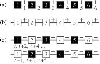
Figure 1: The (a), (b) stationary and (c) periodic states of the opinion dynamics of Eq. 4 in the limit $p_{+}=1$ with synchronous updates. A site $i$ with $\omega_{i}=\pm 1$ is represented by a black (white) square. The spins of the associated Ising model are shown as $+$ or $-$ signs above the links.

Let us first clarify that the variables $\omega_{i}$ cannot directly be interpreted as Ising spins $\sigma_{i}$. For simplicity’s sake, let us assume for a moment that $N$ is even. In the limiting case of $p_{+}=1$, there are two stationary states where all sites have reached either a black or white consensus (Fig. 1a and 1b). For synchronous updates there is, however, also a periodic state where the opinions alternate in space [11]: if all odd sites are black and all even sites white at time $t$, all opinions are inverted at $t+1$ and return to the original state at $t+2$ (Fig. 1c). Unlike in the zero-temperature Ising model, we thus have apparently more than two ground states.

We can, however, establish a connection to the Ising model if we assign spins $\sigma_{i}$ to the $i$-th link (i.e. between the sites $i$ and $i+1$) rather than the sites themselves. We set $\sigma_{i}=1$ if both sites connected by the link agree and $\sigma_{i}=-1$ if they disagree,

$$\sigma_{i}=\omega_{i}\omega_{i+1}.$$ (5)

In terms of $\sigma_{i}$, both consensus states are mapped to maximally positive magnetization, whereas in the alternating state all spins are negative. Thus, the limit $p_{+}=1$ can be mapped to the zero-temperature ferromagnetic Ising model. We will now argue that for any $0<p_{+}<1$, there is a finite-temperature Ising model whose equilibrium properties are those of the original opinion dynamics given by Eq. 4.

3 Mapping the synchronous voter model to an odd or even Ising model

Suppose that the opinions at time $t$ are $\omega_{1}^{(A)},\ldots,\omega_{N}^{(A)}$. What is the probability $\Pr(A\to B)$ to find the opinions $\omega_{1}^{(B)},\ldots,\omega_{N}^{(B)}$ at time $t+1$? Assuming that the probabilities in Eq. 4 are independent for all $i$,

$$\Pr(A\to B)=\prod_{i=1}^{N}\Pr\left[\omega_{i}^{(B)}\bigg{|}\omega_{i-1}^{(A)},\,\omega_{i+1}^{(A)}\right].$$ (6)

We want to show that

$$\frac{\Pr(A\to B)}{\Pr(B\to A)}=e^{\beta(E^{(A)}-E^{(B)})},$$ (7)

where $E^{(A)}$ is the energy of the spins $\sigma_{i}^{(A)}=\omega_{i}^{(A)}\omega_{i+1}^{(A)}$ in the Ising model without magnetic field,

$$E^{(A)}=-J\sum_{i=1}^{N}\sigma_{i}^{(A)}\sigma_{i+1}^{(A)},$$ (8)

and similarly for state $B$. Furthermore,

$$\beta=-\frac{\ln\left(2\sqrt{p_{+}p_{-}}\right)}{2J}$$ (9)

so that every $p_{+}$ can be mapped to a temperature $\left(k_{B}\beta\right)^{-1}$, where $k_{B}$ is the Boltzmann constant. Equation 7 is the detailed balance condition for the Ising model [12]. Consequently, the equilibrium properties of the spins $\sigma_{i}$ can be deduced from the model’s partition function.

Before deriving Eq. 7, we emphasize that not all spin configurations are possible. The number of negative spins must be even; otherwise the opinions $\omega_{i}$ would change an odd number of times as we go once through the chain so that we would not end up with the same opinion with which we started. The restriction to an even number of negative spins changes the partition function of this model compared to the unconstrained Ising model.

First, however, we still need to justify Eq. 7. Let us denote the number of neighbouring spins with opposite signs in states $A$ and $B$ by $n^{(A)}$ and $n^{(B)}$ respectively. Because $E^{(A)}=J\left(2n^{(A)}-N\right)$ and $E^{(B)}=J\left(2n^{(B)}-N\right)$, we can rewrite the right-hand side of Eq. 7 as

$$e^{\beta(E^{(A)}-E^{(B)})}=e^{2\beta J(n^{(A)}-n^{(B)})}.$$ (10)

Because of Eq. 4 and 6, only factors $p_{+}$, $\frac{1}{2}$ and $p_{-}$ can appear in $\Pr(A\to B)$ and $\Pr(B\to A)$,

$$\Pr(A\to B)=p_{+}^{a_{1}}p_{-}^{a_{2}}/2^{a_{3}},$$ (11)

$$\Pr(B\to A)=p_{+}^{b_{1}}p_{-}^{b_{2}}/2^{b_{3}}.$$ (12)

Assuming $p_{+}\neq\frac{1}{2}$, the exponents $a_{i}$, $b_{i}$ are uniquely determined. (If $p_{+}=\frac{1}{2}$ and thus $\beta=0$, Eq. 7 is trivially correct.) There is one factor for each site, so

$$a_{1}+a_{2}+a_{3}=b_{1}+b_{2}+b_{3}=N.$$ (13)

Because $\sigma_{i}\sigma_{i+1}=-1$ if and only if $\omega_{i}+\omega_{i+2}=0$, Eq. 4 implies

$$a_{3}=n^{(A)},$$ (14)

$$b_{3}=n^{(B)}.$$ (15)

From Eq. 4 it also follows that

$$a_{1}-a_{2}=\frac{1}{2}\sum_{i}\omega_{i}^{(B)}\left(\omega_{i-1}^{(A)}+\omega_{i+1}^{(A)}\right),$$ (16)

$$b_{1}-b_{2}=\frac{1}{2}\sum_{i}\omega_{i}^{(A)}\left(\omega_{i-1}^{(B)}+\omega_{i+1}^{(B)}\right).$$ (17)

Splitting the sums and shifting the summation index shows that the sums in Eq. 16 and 17 are equal, thus

$$a_{1}-a_{2}=b_{1}-b_{2}.$$ (18)

Combining Eq. 13, 14, 15 and 18,

$$a_{2}=N-a_{1}-n^{(A)},$$ (19)

$$b_{1}=a_{1}+\frac{1}{2}\left(n^{(A)}-n^{(B)}\right),$$ (20)

$$b_{2}=N-a_{1}-\frac{1}{2}\left(n^{(A)}+n^{(B)}\right),$$ (21)

so that, by plugging into Eq. 11 and 12, we obtain

$$\frac{\Pr(A\to B)}{\Pr(B\to A)}=\left(2\sqrt{p_{+}p_{-}}\right)^{n^{(B)}-n^{(A)}}.$$ (22)

Comparing Eq. 9, 10 and 22 proves Eq. 7.

4 The voter model with random asynchronous updates

Not only the voter model with perfectly synchronous updates of opinions can be mapped to an even or odd Ising model. We will now argue that, by defining the spins as in Eq. 5, we can also interpret asynchronous updates of randomly selected single opinions in terms of an Ising Hamiltonian. While the synchronous case, as shown in the previous section, corresponds to a positive spin interaction $J$ and zero magnetic field $H$, the asynchronous case leads to $J=0$ and, in general, $H\neq 0$ for the following reason.

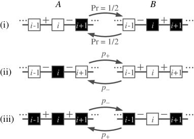
Figure 2: Transition probabilities for asynchronous updates. Depicted are three representative cases where only opinion $i$ changes between states $A$ and $B$. All other cases can be generated by inverting all opinions (from white to black and vice versa) and/or interchanging the order of the chain so that $i-1$ and $i+1$ trade places.

Suppose opinion $\omega_{i}$ is chosen to be updated. The probability to have opinion $\Omega$ in the next time step is given by Eq. 4 while all other opinions remain unchanged. Then the only spins affected are $\sigma_{i-1}$ and $\sigma_{i}$ so that we can ignore the rest of the chain. If $\omega_{i}$ changes between states $A$ and $B$, then we can distinguish the three cases depicted in Fig. 2: either

1. $\Pr(A\to B)=\Pr(B\to A)=\frac{1}{2}$ and $\sigma_{i}^{(A)}+\sigma_{i+1}^{(A)}=\sigma_{i}^{(B)}+\sigma_{i+1}^{(B)}=0$ or

2. $\Pr(A\to B)=p_{+}$ and $\Pr(B\to A)=p_{-}$ and $\sigma_{i}^{(A)}+\sigma_{i+1}^{(A)}=-\sigma_{i}^{(B)}-\sigma_{i+1}^{(B)}=-2$ or

3. $\Pr(A\to B)=p_{-}$ and $\Pr(B\to A)=p_{+}$ and $\sigma_{i}^{(A)}+\sigma_{i+1}^{(A)}=-\sigma_{i}^{(B)}-\sigma_{i+1}^{(B)}=2$.

In summary, we can write all of these cases as

$$\frac{\Pr(A\to B)}{\Pr(B\to A)}=\left(\frac{p_{+}}{p_{-}}\right)^{-\frac{1}{4}\left(\sum\sigma_{i}^{(A)}-\sum\sigma_{i}^{(B)}\right)},$$ (23)

which is of the form of Eq. 7 with the energy $E=-H\sum_{i}\sigma_{i}$ and inverse temperature

$$\beta=\frac{\ln(p_{+}/p_{-})}{4H}.$$ (24)

If $p_{+}\in(\frac{1}{2},1)$, we must have $H>0$ to obtain a positive temperature. Asynchronous opinion updates then tend to favour the states depicted in Fig. 1(a) and (b) where the spins are all positive. Generally, the states in Fig. 1(c) are suppressed when $p_{+}>1/2$ and the dynamic rule mixes synchronous and asynchronous updates (e.g. by updating a fraction of the opinions in every update as in Ref. [13]). The opposite is true for $p_{+}<1/2$ where asynchronous updates generate sequences of alternating opinions and suppress unanimity. All cases, however, have in common that the periodic boundary conditions in the opinions generate an even number of negative spins, resulting in an even (odd) Ising model for even (odd) $N$.

Whether synchronous, asynchronous or partially synchronous updates are more realistic depends on the situation one wishes to model. Asynchronous updates have a long tradition in physics (e.g. the Glauber or Metropolis rules for dynamic Ising models), but synchronous updates, especially in the context of stochastic cellular automata [14], have also been investigated (for example in [15, 16, 17]). If agents can only make decisions at discrete times (e.g. only at the end of a business day or if biological populations exhibit strongly peaked cyclic activity [18]), then synchronous or partially synchronous updates are more applicable. Here we do not intend to argue for any particular update rule. Generally, one has to be humble about social or economic interpretations of such simple rules [19] because true opinion dynamics is far more complex. Our focus here is rather on the model’s structural properties in order to motivate how the even and odd Ising models can arise from another two-state model.

5 Partition function

We denote the partition function for the even and odd Ising model by $Z_{e}$ and $Z_{o}$ respectively,

$$Z_{e}=\sum_{\begin{subarray}{c}\boldsymbol{\sigma}\text{ with}\atop\text{even }N_{+}(\boldsymbol{\sigma})\end{subarray}}e^{-\beta E(\boldsymbol{\sigma})},$$ (25)

$$Z_{o}=\sum_{\begin{subarray}{c}\boldsymbol{\sigma}\text{ with}\atop\text{odd }N_{+}(\boldsymbol{\sigma})\end{subarray}}e^{-\beta E(\boldsymbol{\sigma})}.$$ (26)

If we associate a spin $\sigma_{i}=1$ with the bra vector $\Bra{+1}=(1,0)$ and $\sigma_{i}=-1$ with $\Bra{-1}=(0,1)$, we can write $Z_{e}$ with the transfer matrix of the unconstrained model [20]

$$\mathbf{P}=\left({\begin{array}[]{cc}e^{\beta(J+H)}&e^{-\beta J}\\ e^{-\beta J}&e^{\beta(J-H)}\\ \end{array}}\right)\$$ (29)

as

$$Z_{e}=\sum_{\begin{subarray}{c}\boldsymbol{\sigma}\text{ with}\atop\text{even }N_{+}(\boldsymbol{\sigma})\end{subarray}}\Bra{\sigma_{1}}\mathbf{P}\Ket{\sigma_{2}}\Bra{\sigma_{2}}\mathbf{P}\Ket{\sigma_{3}}\ldots\Bra{\sigma_{N}}\mathbf{P}\Ket{\sigma_{1}}=\Tr\left(\sum_{\begin{subarray}{c}\boldsymbol{\sigma}\text{ with}\atop\text{even }N_{+}(\boldsymbol{\sigma})\end{subarray}}\Ket{\sigma_{1}}\Bra{\sigma_{1}}\mathbf{P}\ldots\Ket{\sigma_{N}}\Bra{\sigma_{N}}\mathbf{P}\right).$$ (30)

Similarly,

$$Z_{o}=\Tr\left(\sum_{\begin{subarray}{c}\boldsymbol{\sigma}\text{ with}\atop\text{odd }N_{+}(\boldsymbol{\sigma})\end{subarray}}\Ket{\sigma_{1}}\Bra{\sigma_{1}}\mathbf{P}\ldots\Ket{\sigma_{N}}\Bra{\sigma_{N}}\mathbf{P}\right).$$ (31)

Let us define

$$\mathbf{M}_{e}=\sum_{\begin{subarray}{c}\boldsymbol{\sigma}\text{ with}\atop\text{even }N_{+}(\boldsymbol{\sigma})\end{subarray}}\Ket{\sigma_{1}}\Bra{\sigma_{1}}\mathbf{P}\ldots\Ket{\sigma_{N}}\Bra{\sigma_{N}}\mathbf{P},$$ (32)

$$\mathbf{M}_{o}=\sum_{\begin{subarray}{c}\boldsymbol{\sigma}\text{ with}\atop\text{odd }N_{+}(\boldsymbol{\sigma})\end{subarray}}\Ket{\sigma_{1}}\Bra{\sigma_{1}}\mathbf{P}\ldots\Ket{\sigma_{N}}\Bra{\sigma_{N}}\mathbf{P}.$$ (33)

Induction on $N$ proves

$$\left({\begin{array}[]{cc}\mathbf{M}_{e},&\mathbf{M}_{o}\\ \mathbf{M}_{o},&\mathbf{M}_{e}\\ \end{array}}\right)=\left({\begin{array}[]{cc}\Ket{-1}\Bra{-1}\mathbf{P},&\Ket{+1}\Bra{+1}\mathbf{P}\\ \Ket{+1}\Bra{+1}\mathbf{P},&\Ket{-1}\Bra{-1}\mathbf{P}\\ \end{array}}\right)^{N}.$$ (38)

With the definition

$$\mathbf{Q}=\left({\begin{array}[]{cc}\Ket{-1}\Bra{-1}\mathbf{P},&\Ket{+1}\Bra{+1}\mathbf{P}\\ \Ket{+1}\Bra{+1}\mathbf{P},&\Ket{-1}\Bra{-1}\mathbf{P}\\ \end{array}}\right)=\left({\begin{array}[]{cccc}0&0&e^{\beta(J+H)}&e^{-\beta J}\\ e^{-\beta J}&e^{\beta(J-H)}&0&0\\ e^{\beta(J+H)}&e^{-\beta J}&0&0\\ 0&0&e^{-\beta J}&e^{\beta(J-H)}\\ \end{array}}\right)$$ (45)

we can write

$$Z_{e}=\Tr\left(\mathbf{M}_{e}\right)=\frac{1}{2}\Tr\left(\mathbf{Q}^{N}\right).$$ (47)

To simplify the notation further, we introduce

$$x=\beta H,$$ (48)

$$y=\beta J.$$ (49)

The eigenvalues of $\mathbf{Q}$ are then

$$\lambda_{1,2}=e^{y}\left(\cosh x\pm\sqrt{\sinh^{2}x+e^{-4y}}\right),$$ (50)

$$\lambda_{3,4}=e^{y}\left(-\sinh x\pm\sqrt{\cosh^{2}x-e^{-4y}}\right).$$ (51)

Consequently,

$$Z_{e}=\frac{1}{2}\left(\lambda_{1}^{N}+\lambda_{2}^{N}+\lambda_{3}^{N}+\lambda_{4}^{N}\right).$$ (52)

We can derive $Z_{o}$ as follows. The eigenvalues $\lambda_{1,2}$ are also the eigenvalues of $\mathbf{P}$ and therefore the partition function of the unconstrained Ising model is $Z_{u}=\lambda_{1}^{N}+\lambda_{2}^{N}$. Moreover $Z_{u}=Z_{e}+Z_{o}$ so that

$$Z_{o}=\frac{1}{2}\left(\lambda_{1}^{N}+\lambda_{2}^{N}-\lambda_{3}^{N}-\lambda_{4}^{N}\right).$$ (53)

Because $\lambda_{1}$ is the leading eigenvalue, we find in the thermodynamic limit (i.e. $N\to\infty$) with fixed $x$ and $y$ that $Z_{e}\propto Z_{o}\propto Z_{u}\propto\lambda_{1}^{N}$. As a consequence, all equilibrium properties of the even and odd Ising models converge to the same limits as the unconstrained model. However, we will analytically derive in Sec. 9 different scaling limits for $N\to\infty$ when temperature and magnetic field go to their critical value (i.e. zero) such that $Ne^{-2y}$ and $N\sinh x$ are asymptotically constants. For this purpose, it will be instructive to derive first some exact formulae for finite $N$.

6 Magnetization and Susceptibility

We first calculate the mean magnetization per spin

$$\langle m\rangle\equiv\frac{\langle\sum_{i}\sigma_{i}\rangle}{N}=\frac{1}{N}\frac{\partial}{\partial x}\ln Z,$$ (54)

where $Z$ is the partition function of the model in question and the angle brackets denote the ensemble average. With the auxiliary functions

$$s_{1}(x,y)=\frac{\sinh x}{\sqrt{\sinh^{2}x+e^{-4y}}},$$ (55)

$$c_{1}(x,y)=\frac{\cosh x}{\sqrt{\cosh^{2}x-e^{-4y}}},$$ (56)

we can write Eq. 54 as

$$\langle m\rangle_{e,o}(x,y)=\frac{s_{1}\left(\lambda_{1}^{N}-\lambda_{2}^{N}\right)\mp c_{1}\left(\lambda_{3}^{N}-\lambda_{4}^{N}\right)}{\lambda_{1}^{N}+\lambda_{2}^{N}\pm\lambda_{3}^{N}\pm\lambda_{4}^{N}},$$ (57)

where the upper signs apply to the even and the lower signs to the odd model.

In the special case $x=0$, applicable to the synchronous voter model, we insert the eigenvalues from Eq. 50 and 51 (Fig. 3a)

$$\langle m\rangle_{e,o}(x=0,y)=\begin{cases}\langle m\rangle_{u}(x=0,y)=0&\text{if $N$ is even},\\ \mp\frac{e^{y}}{\cosh^{N}y+\sinh^{N}y}\left(\frac{\sinh(2y)}{2}\right)^{(N-1)/2}&\text{if $N$ is odd.}\end{cases}$$ (58)

Hence, for odd $N$, even when there is no external magnetic field (i.e. $H=0$), the magnetization is generally different from zero. This phenomenon can be intuitively explained. The constraint of an even number of positive spins prevents for odd $N$ a ground state with perfectly aligned positive spins. However, the state with $\sigma_{1}=\ldots=\sigma_{N}=-1$ is permitted and therefore the mean magnetization in the limit $y\to\infty$ is $-1$. The same argument applies with opposite signs to the odd model. In the antiferromagnetic limit (i.e. $y\to-\infty$) the neighbouring spins prefer to be in opposite directions, but an odd $N$ forces at least one pair to point in the same direction and thus $m_{e,o}=(-1)^{(N\pm 1)/2}/N$.

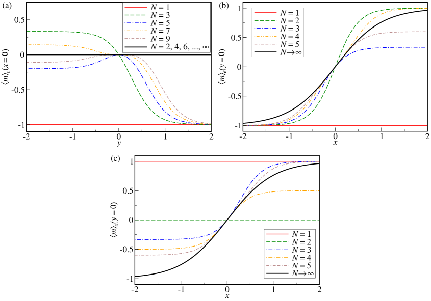
Figure 3: The mean magnetization $\langle m_{e}\rangle$ (a) as a function of $y$ when $x=0$, (b) as a function of $x$ when $y=0$. (c) The mean magnetization $\langle m_{o}\rangle$ for $y=0$.

The relevant case for the asynchronous voter model is $y=0$ where the interactions between spins are negligible compared to the external magnetic field,

$$\langle m\rangle_{e,o}(x,y=0)=\frac{\sinh(2x)}{2}\times\frac{\cosh^{N-2}x\pm(-1)^{N}\sinh^{N-2}x}{\cosh^{N}x\pm(-1)^{N}\sinh^{N}x}.$$ (59)

The functions are plotted in Fig. 3(b) and (c). In the unconstrained model the magnetization $\langle m\rangle_{u}(x,y=0)=\tanh x$ is independent of $N$. However, in the even and odd models, the constraints on the number of spins acts as an effective interaction so that the partition function does not factorize although $J=0$. Consequently, the magnetization of Eq. 59 depends on $N$.

The fluctuations in the magnetization are measured by the susceptibility per spin

$$\chi\equiv\beta N\left(\langle m^{2}\rangle-\langle m\rangle^{2}\right)=\frac{\partial\langle m\rangle}{\partial H}.$$ (60)

Taking the derivative of Eq. 57 for general $x$ and $y$ is in principle possible, but leads to rather lengthy expressions. We focus here instead directly on the two special cases $x=0$ and $y=0$.

For $x=0$ (i.e. in the absence of an external magnetic field),

$$\chi_{e,o}(x=0,y)=\begin{cases}\frac{\beta e^{2y}\left(\cosh^{N}y-\sinh^{N}y\pm 2^{-N/2}N\sinh^{N/2-1}(2y)\right)}{\left(\cosh^{N/2}y\pm\sinh^{N/2}y\right)^{2}}&\text{if $N$ is even,}\\ \frac{\beta e^{2y}\left(\cosh^{2N}y-\sinh^{2N}y-2^{1-N}N\sinh^{N-1}(2y)\right)}{\left(\cosh^{N}y+\sinh^{N}y\right)^{2}}&\text{if $N$ is odd,}\end{cases}$$ (61)

compared to $\chi_{u}=\beta e^{2y}(\cosh^{N}y-\sinh^{N}y)/(\cosh^{N}y+\sinh^{N}y)$. Plotting $\chi_{e,o}$ in Fig. 4a and 4b, the most striking feature for odd $N$ is $\lim_{y\to\infty}\chi_{e,o}=0$, whereas the unconstrained Ising model (and the even model for even $N$) reaches in this limit its maximum susceptibility $\beta N$. The reason is that, as already mentioned, the even and odd models for odd $N$ only have one ground state each, but the unconstrained model has two.

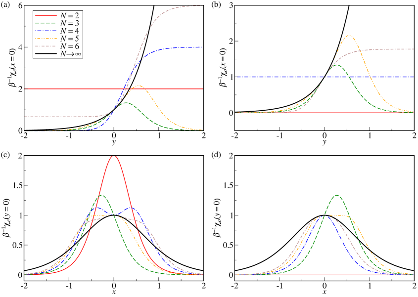
Figure 4: The susceptibility $\chi$ divided by the inverse temperature $\beta$ for (a), (b) zero magnetic field $H$ as a function of $y=\beta J$ and (c), (d) zero spin interaction $J$ as a function of $x=\beta H$. Panels (a) and (c) show the results for the even Ising model, (b) and (d) for the odd model.

For the odd model with even $N$ we observe yet another interesting phenomenon. The susceptibility reaches its maximum in the limit $y\to\infty$, but with a smaller value than the unconstrained or even models, namely $\lim_{y\to\infty}\chi_{o}=\beta(N^{2}-4)/(3N)$. The explanation is that the perfectly aligned ground states of the unconstrained models are not permitted. Therefore, the states of minimum energy in the odd model are the first excited states of the unconstrained model whose magnetization is not confined to the extreme values $m=\pm 1$.

In the case of no internal interactions (i.e. $y=0$),

$$\chi_{e,o}(x,y=0)=\beta\left(\frac{\cosh^{N-2}x\mp(-1)^{N}\sinh^{N-2}x}{\cosh^{N}x\pm(-1)^{N}\sinh^{N}x}\pm\frac{(-1)^{N}N\sinh^{N-2}(2x)}{2^{N-2}\left(\cosh^{N}x\pm(-1)^{N}\sinh^{N}x\right)^{2}}\right),$$ (62)

while $\chi_{u}=\beta\cosh^{-2}x$. We plot $\chi_{e,o}$ in Fig. 4c and 4d. For odd $N$, they satisfy $\chi_{e}(x,0)=\chi_{o}(-x,0)$ because in this case the odd model is equivalent to the even model with flipped signs of spins and magnetic field. If $N$ is even, $\chi_{e}$ and $\chi_{o}$ are intrinsically symmetric, but with larger values in the tails of the even model because $\chi_{e}/\chi_{o}\to 3N/(N-2)$ as $|x|\to\infty$ and $y=0$.

7 Nearest-neighbour correlations, internal energy and heat capacity

If we replace in Eq. 54 the partial derivative with respect to $x$ by differentiation with respect to $y$, we obtain the mean nearest-neighbour correlation

$$\langle g_{1}\rangle\equiv\frac{1}{N}\left\langle\sum_{i}\sigma_{i}\sigma_{i+1}\right\rangle=\frac{1}{N}\frac{\partial}{\partial y}\ln Z.$$ (63)

If we define the functions

$$s_{2}(x,y)=2e^{-3y}\left(\sinh^{2}x+e^{-4y}\right)^{-1/2},$$ (64)

$$c_{2}(x,y)=2e^{-3y}\left(\cosh^{2}x-e^{-4y}\right)^{-1/2},$$ (65)

then

$$\langle g_{1}\rangle_{e,o}(x,y)=1+\frac{s_{2}\left(\lambda_{2}^{N-1}-\lambda_{1}^{N-1}\right)\pm c_{2}\left(\lambda_{3}^{N-1}-\lambda_{4}^{N-1}\right)}{\lambda_{1}^{N}+\lambda_{2}^{N}\pm\lambda_{3}^{N}\pm\lambda_{4}^{N}}.$$ (66)

Without external magnetic field,

$$\langle g_{1}\rangle {}_{e,o}(x=0,y)= \begin{cases}1-\frac{\cosh^{N/2-1}y\mp\sinh^{N/2-1}y}{e^{y}\left(\cosh^{N/2}y\pm\sinh^{N/2}y\right)}&\text{if $N$ is even},\\ \langle g_{1}\rangle_{u}(x=0,y)=1+\frac{\sinh^{N-1}y-\cosh^{N-1}y}{e^{y}\left(\cosh^{N}y+\sinh^{N}y\right)}&\text{if $N$ is odd}.\end{cases}$$ (67)

If $N$ is odd, $\langle g_{1}\rangle_{e,o}(x=0,y)$ is equal to the correlation in the unconstrained model for the following reason. The spin configurations in the unconstrained model can be divided into two sets: one set containing all configurations of the even model and another set with all odd-numbered states. We can map every element in one set uniquely to the configuration in the other set that has all spins inverted. Because the sum of Eq. 63 is invariant if all spins are simultaneously flipped, the average correlations must be equal in both sets. The same argument cannot be applied to even $N$, however, because inverting the spins in the even or odd set generates another spin in the same set. As a consequence, $\langle g_{1}\rangle_{e}$ and $\langle g_{1}\rangle_{o}$ are in this case different functions.

With a magnetic field, but with vanishing spin interactions,

$$\langle g_{1}\rangle_{e,o}(x,y=0)=1-\frac{\cosh^{N-2}x\mp(-1)^{N}\sinh^{N-2}x}{\cosh^{N}x\pm(-1)^{N}\sinh^{N}x},$$ (68)

compared to $\langle g_{1}\rangle_{u}=\tanh^{2}x$. For odd $N$, we find $\langle g_{1}\rangle_{e}(x,0)=\langle g_{1}\rangle_{o}(-x,0)$ for the same reason as discussed after the corresponding Eq. 62 for the susceptibility. We also find again that, for even $N$, $\langle g_{1}\rangle_{e}(x,0)=\langle g_{1}\rangle_{e}(-x,0)$ and $\langle g_{1}\rangle_{o}(x,0)=\langle g_{1}\rangle_{o}(-x,0)$. Expanding Eq. 68, however, shows that the limits for $|x|\to\infty$ and even $N$ are different: $\langle g_{1}\rangle_{e}\to 1$, but $\langle g_{1}\rangle_{o}\to 1-4/N$. The intuition behind this result is that a strong magnetic field can perfectly align the spins in the even, but not in the odd model.

Closely related to the nearest-neighbour correlations is the internal energy (i.e. ensemble average of the Hamiltonian) per spin

$$U\equiv\frac{\langle E\rangle}{N}=-\frac{1}{N}\frac{\partial}{\partial\beta}\ln Z.$$ (69)

In general, the calculation yields rather lengthy expressions. However, if $H=0$, then $U_{e,o}=-J\langle g_{1}\rangle_{e,o}(x=0,y)$. If, on the other hand, $J$ vanishes, then $U_{e,o}=-H\langle m\rangle_{e,o}(x,y=0)$. Using our earlier results of Eq. 59 and 67,

$$U_{e,o}(x=0,y)=\begin{cases}J\left(\frac{\cosh^{N/2-1}y\mp\sinh^{N/2-1}y}{e^{y}\left(\cosh^{N/2}y\pm\sinh^{N/2}y\right)}-1\right)&\text{if $N$ is even},\\ U_{u}(x=0,y)=J\left(\frac{\cosh^{N-1}y-\sinh^{N-1}y}{e^{y}\left(\cosh^{N}y+\sinh^{N}y\right)}-1\right)&\text{if $N$ is odd},\end{cases}$$ (70)

$$U {}_{e,o}(x,y=0)= -\frac{H\sinh(2x)}{2}\times\frac{\cosh^{N-2}x\pm(-1)^{N}\sinh^{N-2}x}{\cosh^{N}x\pm(-1)^{N}\sinh^{N}x},$$ (71)

while $U_{u}(x,y=0)=-H\tanh x$.

Taking another derivative of $\ln Z$ with respect to $\beta$ gives us the heat capacity per spin, which measures the fluctuations in the energy,

$$C\equiv\frac{k_{B}\beta^{2}}{N}\left(\langle E^{2}\rangle-\langle E\rangle^{2}\right)=-k_{B}\beta^{2}\frac{\partial U}{\partial\beta}.$$ (72)

For vanishing $H$, we can use $(\partial U)/(\partial\beta)=J(\partial U)/(\partial y)$ and Eq. 70. If $J=0$, then $C=k_{B}\beta H^{2}\chi$, so the heat capacity follows directly from Eq. 62,

$$C_{e,o}(x=0,y)=$$ (73)

$$\hskip 14.22636pt\begin{cases}\frac{k_{B}\beta^{2}J^{2}}{\cosh^{N/2}y\pm\sinh^{N/2}y}\left(\cosh^{N/2-2}y\mp\sinh^{N/2-2}y\pm\frac{N\sinh^{N/2-2}(2y)}{2^{N/2-1}\left(\cosh^{N/2}y\pm\sinh^{N/2}y\right)}\right)&\text{if $N$ is even,}\\ C_{u}(x=0,y)=\frac{k_{B}\beta^{2}J^{2}}{\cosh^{N}y+\sinh^{N}y}\left(\cosh^{N-2}y-\sinh^{N-2}y+\frac{N\sinh^{N-2}(2y)}{2^{N-2}\left(\cosh^{N}y+\sinh^{N}y\right)}\right)&\text{if $N$ is odd,}\end{cases}$$

$$C_{e,o}(x,y=0)=$$ (74)

$$\hskip 14.22636ptk_{B}\beta^{2}H^{2}\left(\frac{\cosh^{N-2}x\mp(-1)^{N}\sinh^{N-2}x}{\cosh^{N}x\pm(-1)^{N}\sinh^{N}x}\pm\frac{(-1)^{N}N\sinh^{N-2}(2x)}{2^{N-2}\left(\cosh^{N}x\pm(-1)^{N}\sinh^{N}x\right)^{2}}\right),$$

approaching $C_{u}(x=0,y)=k_{B}\beta^{2}H^{2}\cosh^{-2}(x)$ in the thermodynamic limit.

8 Correlation function

We can generalize the calculation in the previous section to find the correlation between $k$-th nearest neighbours. For this purpose we make the spin interactions $J$ in an auxiliary Hamiltonian $\tilde{E}$ dependent on the position $i$, but for simplicity’s sake we drop the magnetic field,

$$\tilde{E}(\boldsymbol{\sigma})=-\sum_{i=1}^{N}{J_{i}\sigma_{i}\sigma_{i+1}}.$$ (75)

Applying the same line of reasoning that led us to Eq. 47, we can show that the partition function for the Hamiltonian $\tilde{E}$ in the case of even $N^{+}$ is

$$\tilde{Z}_{e}=\frac{1}{2}\Tr\left(\prod_{i=1}^{N}\mathbf{Q}_{i}\right),$$ (76)

where

$$\mathbf{Q}_{i}= \left({\begin{array}[]{cccc}0&0&e^{\beta J_{i}}&e^{-\beta J_{i}}\\ e^{-\beta J_{i}}&e^{\beta J_{i}}&0&0\\ e^{\beta J_{i}}&e^{-\beta J_{i}}&0&0\\ 0&0&e^{-\beta J_{i}}&e^{\beta J_{i}}\\ \end{array}}\right)$$ (81)

plays the role of the transfer matrix of Eq. 45. The matrices $\mathbf{Q}_{i}$ do not commute and therefore we cannot simultaneously diagonalize them for computing the trace in Eq. 76. However, the product $\mathbf{Q}_{i}\mathbf{Q}_{i+1}$ commutes with $\mathbf{Q}_{i+2}\mathbf{Q}_{i+3}$. These products are diagonalized as $\mathbf{R}\mathbf{Q}_{i}\mathbf{Q}_{i+1}\mathbf{R}$ by the matrix of eigenvectors

$$\mathbf{R}=\frac{1}{2}\left({\begin{array}[]{rrrr}1&1&1&1\\ 1&-1&1&-1\\ 1&1&-1&-1\\ 1&-1&-1&1\\ \end{array}}\right)=\mathbf{R}^{-1},$$ (86)

and the corresponding eigenvalues are

$$\left(\mathbf{R}\mathbf{Q}_{i}\mathbf{Q}_{i+1}\mathbf{R}\right)_{11}=4\cosh(\beta J_{i})\cosh(\beta J_{i+1}),$$ (87)

$$\left(\mathbf{R}\mathbf{Q}_{i}\mathbf{Q}_{i+1}\mathbf{R}\right)_{22}=4\sinh(\beta J_{i})\sinh(\beta J_{i+1}),$$ (88)

$$\left(\mathbf{R}\mathbf{Q}_{i}\mathbf{Q}_{i+1}\mathbf{R}\right)_{33}=4\sinh(\beta J_{i})\cosh(\beta J_{i+1}),$$ (89)

$$\left(\mathbf{R}\mathbf{Q}_{i}\mathbf{Q}_{i+1}\mathbf{R}\right)_{44}=4\cosh(\beta J_{i})\sinh(\beta J_{i+1}).$$ (90)

If $N$ is even, it follows that

$$\tilde{Z}_{e,\text{ even $N$}}=2^{N-1}\bigg{(}\prod_{i=1}^{N}\cosh(\beta J_{i})+\prod_{i=1}^{N}\sinh(\beta J_{i})+$$ (91)

$$\hskip 14.22636pt\prod_{i=1}^{N/2}\cosh(\beta J_{2i-1})\sinh(\beta J_{2i})+\prod_{i=1}^{N/2}\sinh(\beta J_{2i-1})\cosh(\beta J_{2i})\bigg{)},$$

while for odd $N$ the partition function is half of the unconstrained model’s partition function

$$\tilde{Z}_{e,\text{ odd $N$}}=\frac{1}{2}\tilde{Z}_{u}=2^{N-1}\left(\prod_{i=1}^{N}\cosh(\beta J_{i})+\prod_{i=1}^{N}\sinh(\beta J_{i})\right).$$ (92)

For the odd model, we can apply $\tilde{Z}_{o}=\tilde{Z}_{u}-\tilde{Z_{e}}$. The disconnected correlation function $\langle g_{k}\rangle$ can now be computed as

$$\langle g_{k}\rangle=\frac{1}{N}\left\langle\sum_{i}\sigma_{i}\sigma_{i+k}\right\rangle=\left[\frac{1}{\beta^{k}\tilde{Z}}\frac{\partial}{\partial J_{1}}\frac{\partial}{\partial J_{2}}\ldots\frac{\partial}{\partial J_{k}}\tilde{Z}\right]_{J_{1}=\ldots=J_{N}=J}$$ (93)

with the final result

$$\langle g_{k}\rangle_{e,o}=\begin{cases}\frac{\cosh^{N-k}y\sinh^{k}y+\sinh^{N-k}y\cosh^{k}y\pm 2^{1-N/2}\cosh(2y)\sinh^{N/2-1}(2y)}{\left(\cosh^{N/2}y\pm\sinh^{N/2}y\right)^{2}}&\text{if $N$ even, $k$ odd,}\\ \frac{\cosh^{N-k}y\sinh^{k}y+\sinh^{N-k}y\cosh^{k}y\pm 2^{1-N/2}\sinh^{N/2}(2y)}{\left(\cosh^{N/2}y\pm\sinh^{N/2}y\right)^{2}}&\text{if $N$ even, $k$ even,}\\ \langle g_{k}\rangle_{u}=\frac{\cosh^{N-k}y\,\sinh^{k}y+\sinh^{N-k}y\,\cosh^{k}y}{\cosh^{N}y+\sinh^{N}y}&\text{if $N$ odd}.\end{cases}\rule[-15.00002pt]{10.0pt}{0.0pt}$$ (94)

Taking the limit $N\to\infty$ while keeping $y$ and $k$ fixed, all three cases have the same asymptotic value $\lim_{N\to\infty}\langle g_{k}\rangle_{e,o,u}=\tanh^{k}y$ and the correlation length is hence $\xi=-[\ln(\tanh y)]$. The divergence at $y=0$ can be expressed as a power law in the reduced temperature [21]

$$T_{r}=e^{-2y}$$ (95)

because near $T_{r}=0$

$$\xi\approx{2T_{r}}^{-1}\propto T_{r}^{-\nu},$$ (96)

where the critical correlation length exponent satisfies $\nu=1$ in the unconstrained, even and odd model.

9 Approach to the thermodynamic limit

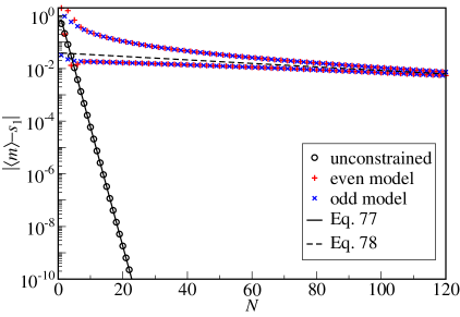
Figure 5: The difference between the magnetization $\langle m\rangle$ and $s_{1}$ for a finite chain of length $N$, $x=0.5$ and $y=1$. We note that $s_{1}$, defined in Eq. 55, is the thermodynamic limit of $\langle m\rangle$. Circles, $+$ and $\times$ symbols are exact results. The solid and dashed lines are the leading-order approximations of Eq. 98 and 99. The constrained models converge much more slowly than their unconstrained counterpart.

It is not surprising that $\nu$ does not depend on whether we constrain the number of positive spins to even or odd values or have no such constraint. We have already pointed out the reason after Eq. 53: the thermodynamic limit at fixed temperature is determined by the leading eigenvalue $\lambda_{1}$, and this eigenvalue is common to the transfer matrices $\mathbf{P}$ and $\mathbf{Q}$. The leading-order correction to the magnetization, however, depends on the eigenvalue with the second largest absolute value. If we call this eigenvalue $\lambda_{s}$, then the average magnetization for a chain of length $N$ behaves asymptotically as

$$\langle m\rangle=s_{1}+\left(\frac{\lambda_{s}}{\lambda_{1}}\right)^{N-1}\frac{\partial}{\partial x}\left(\frac{\lambda_{s}}{\lambda_{1}}\right)+\text{higher order terms},$$ (97)

obtained by expanding the logarithm in Eq. 54 and inserting the definition of $s_{1}$ from Eq. 55. In the unconstrained case we have $\lambda_{s}=\lambda_{2}$, but for the constrained models one of the other two eigenvalues of the matrix $\mathbf{Q}$ has a larger absolute value so long as $x\neq 0$ or $y\neq 0$. For example, if $x$ and $y$ are both positive, then $\lambda_{s}=\lambda_{4}$ and the leading-order corrections for the unconstrained, even and odd models are

$$\langle m\rangle_{u}-s_{1}=-2s_{1}\left(\frac{\lambda_{2}}{\lambda_{1}}\right)^{N},$$ (98)

$$\langle m\rangle_{e}-s_{1}=-\langle m\rangle_{o,N}+s_{1}=(c_{1}-s_{1})\left(\frac{\lambda_{4}}{\lambda_{1}}\right)^{N},$$ (99)

respectively (see Eq. 56 for the definition of $c_{1}$). In general, $|\lambda_{4}|$ is considerably larger than $|\lambda_{2}|$. As a consequence, the leading-order correction decays much more slowly in the constrained cases than in the unconstrained one (Fig. 5).

The difference in the asymptotic approach to the thermodynamic limit becomes even more apparent if we take the limit $N\to\infty$ while simultaneously $J\to\infty$ (so that $T_{r}\to 0$) and $H\to 0$ (so that $x\to 0$) in such a way that the products

$$t\equiv NT_{r},$$ (100)

$$h\equiv N\sinh x$$ (101)

are constants. In the thermodynamic limit the magnetic field $H$ scales $\propto N^{-1}$. We could have alternatively defined $h=Nx$ to make this inverse proportionality more apparent, but the definition of Eq. 101 is a little bit more convenient when substituting the hyperbolic functions in Eq. 50 and 51. After applying the formula $\lim_{N\to\infty}(1+z/N)^{N}=e^{z}$ to Eq. 52 and Eq. 53, we obtain the partition functions for large $N$,

$$Z_{u}=2N^{N/2}t^{-N/2}\cosh\sqrt{h^{2}+t^{2}},$$ (102)

$$Z_{e,o}=\begin{cases}N^{N/2}t^{-N/2}\left(\cosh\sqrt{h^{2}+t^{2}}\pm\cosh h\right)&\text{if $N$ is even},\\ N^{N/2}t^{-N/2}\left(\cosh\sqrt{h^{2}+t^{2}}\mp\sinh h\right)&\text{if $N$ is odd}.\end{cases}$$ (103)

All thermodynamic quantities can now be derived from the partition function by taking the appropriate derivatives, for example $\langle m\rangle=\partial(\ln Z)/\partial h$. Alternatively, we can also take the thermodynamic limits of Eq. 57, 61 and 73. We tabulate the results in Table 1.

	unconstrained	even model	odd model
$\langle m\rangle$	$\frac{h\tanh\sqrt{h^{2}+t^{2}}}{\sqrt{h^{2}+t^{2}}}$	$\frac{\frac{h}{\sqrt{h^{2}+t^{2}}}\sinh\sqrt{h^{2}+t^{2}}+\sinh h}{\cosh\sqrt{h^{2}+t^{2}}+\cosh h}$	$\frac{\frac{h}{\sqrt{h^{2}+t^{2}}}\sinh\left(\sqrt{h^{2}+t^{2}}\right)-\sinh h}{\cosh\left(\sqrt{h^{2}+t^{2}}\right)-\cosh h}$ if $N$ is even,
		$\frac{\frac{h}{\sqrt{h^{2}+t^{2}}}\sinh\sqrt{h^{2}+t^{2}}-\cosh h}{\cosh\sqrt{h^{2}+t^{2}}-\sinh h}$	$\frac{\frac{h}{\sqrt{h^{2}+t^{2}}}\sinh\left(\sqrt{h^{2}+t^{2}}\right)+\cosh h}{\cosh\left(\sqrt{h^{2}+t^{2}}\right)+\sinh h}$ if $N$ is odd.
$\frac{\chi(h=0)}{\beta}$	$\frac{N\tanh t}{t}$	$N\left(\frac{\tanh\left(\frac{t}{2}\right)}{t}+\frac{1}{2\cosh^{2}\left(\frac{t}{2}\right)}\right)$	$N\left(\frac{\coth\left(\frac{t}{2}\right)}{t}-\frac{1}{2\sinh^{2}\left(\frac{t}{2}\right)}\right)$ if $N$ is even,
		$N\left(\frac{\tanh t}{t}-\frac{1}{\cosh^{2}t}\right)$ if $N$ is odd.
$\frac{C(h=0)}{k_{B}\beta^{2}J^{2}}$	$\frac{4t}{N}\left(\tanh t+\frac{t}{\cosh^{2}t}\right)$	$\frac{2t}{N}\left(2\tanh\left(\frac{t}{2}\right)+\frac{t}{\cosh^{2}\left(\frac{t}{2}\right)}\right)$	$\frac{2t}{N}\left(2\coth\left(\frac{t}{2}\right)-\frac{t}{\sinh^{2}\left(\frac{t}{2}\right)}\right)$ if $N$ is even
		$\frac{4t}{N}\left(\tanh t+\frac{t}{\cosh^{2}t}\right)$ if $N$ is odd.

Table 1: Thermodynamic properties for $N\to\infty$ and constant $t$, $h$ (defined in Eq. 100 and 101).

It is instructive to compare these equations with the canonical finite-size scaling forms, for example for the susceptibility

$$\chi(h=0) \propto N^{\gamma/\nu}f_{\chi}(N^{1/\nu}t).$$ (104)

While we find that $\gamma=\nu=1$ for all of the cases listed in Table 1 (see also our remark after Eq. 96), the scaling functions $f_{\chi}$ (plotted in Fig. 6) are fundamentally different.

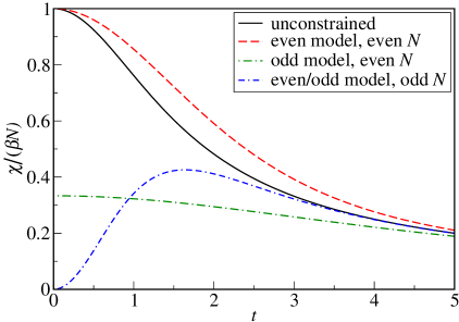
Figure 6: The scaling function of the susceptibility $\chi(h=0)$ in the limit $N\to\infty$, $\beta\to\infty$ with finite $t=Ne^{-2\beta J}$. The scaling functions for the unconstrained, even and odd models exhibit different behaviour, especially if $t$ is small.

10 The probability distribution of the magnetization

Because of the differences between the unconstrained, even and odd models in Table 1, one may wonder how the probability distribution of the magnetization [22, 23, 24, 25] differs; after all, $\langle m\rangle$ and $\chi$ are essentially the mean and variance of this distribution. We repeat here the arguments developed by Antal et al. [26] for the unconstrained model with zero magnetic field. We denote the total magnetization by $M\equiv\sum_{i}\sigma_{i}$ and the number of domain walls (i.e. boundaries between stretches of contiguous positive and negative spins) by $2d$; it must be an even number because of the periodic boundary conditions. The main task is to count the number $\Omega(d,M)$ of configurations with $2d$ domain walls and magnetization $M$. Their probability $P(d,M)$ in thermal equilibrium with $H=0$ will then follow from

$$P(d,M)=\frac{e^{(N-4d)y}}{Z}\Omega(d,M),$$ (105)

whose marginal distribution

$$P(M)=\sum_{d}P(d,M)$$ (106)

is the probability distribution we are looking for.

We can find $\Omega(d,M)$ with the following combinatorial argument. Let us assume that there are $N_{+}$ positive and $N_{-}=N-N_{+}$ negative spins, and that the first spin is positive. We could for example have

$$\underbrace{w_{0}+}++\underbrace{w_{1}-}---\underbrace{w_{2}+}++\ldots++\underbrace{w_{2d-1}-}w_{2d}+++,$$ (107)

where we marked the positions of the domain walls by $w_{1},\ldots,w_{2d}$. At the periodic boundary between the first and last spin there may not be a domain wall (in the example above there is not), but we will always symbolically put $w_{0}$ in front of the chain. We now mentally glue $w_{0},\ldots,w_{2d-1}$ to the next spin in the chain (indicated by the braces in Eq. 107). In this manner, $d$ negative spins are attached to domain walls, whereas the remaining $N_{-}-d$ can be freely placed in the $d$ negative domains. The well-known stars-and-bars theorem [27] implies that there are $\bigl{(}\begin{smallmatrix}N_{-}-1\\ d-1\end{smallmatrix}\bigr{)}$ different ways to distribute the negative spins.

The positive spins require a little more care, because there may not be a positive spin trailing the domain wall $w_{2d}$. We can account for this exception by not attaching $w_{2d}$ to the following spin. There are thus $d$ positive spins attached to $w_{0},w_{2},\ldots,w_{2d-2}$, while the remaining $N_{+}-d$ positive spins can be freely distributed into $d+1$ segments, namely the positive intervals following $w_{0},w_{2},\ldots,w_{2d}$. According to the stars-and-bars theorem, there are $\bigl{(}\begin{smallmatrix}N_{+}\\ d\end{smallmatrix}\bigr{)}$ different possibilities.

Because the positive and negative spins are placed independently of each other, the number of configurations is simply the product of the binomial coefficients $\bigl{(}\begin{smallmatrix}N_{-}-1\\ d-1\end{smallmatrix}\bigr{)}\bigl{(}\begin{smallmatrix}N_{+}\\ d\end{smallmatrix}\bigr{)}$. If we had started the chain with a negative spin, we would have obtained the same expression with the subscripts $+$ and $-$ interchanged, so that

$$\Omega(d,M)=\binom{N_{-}-1}{d-1}\binom{N_{+}}{d}+\binom{N_{+}-1}{d-1}\binom{N_{-}}{d}.$$ (108)

This expression from Antal et al. [26] is equally valid for the unconstrained, even and odd model. The constraints only enter in the permitted values for $M$ whose consequence becomes apparent when we take the continuum limit. To this end, we take $N\to\infty$ for a fixed value of $d$ and write $m=M/N$, so that

$$\Omega(d,m)=\frac{N^{2d-1}}{2^{2d-2}\,d!\,(d-1)!}\left(1-m^{2}\right)^{d-1}.$$ (109)

For the time being let us assume that $|m|\neq 1$ and thus $d\neq 0$. We can insert Eq. 109 into Eq. 105 and 106, but have to bear in mind that changing from the discrete variable $M$ to the continuous variable $m$ generates an additional prefactor, which we will call $N/\Delta_{M}$,

$$P(m)=\frac{4N^{N/2}}{t^{N/2}\Delta_{M}Z(1-m^{2})}\sum_{d=1}^{\infty}\frac{t^{2d}(1-m^{2})^{d}}{2^{2d}d!(d-1)!}.$$ (110)

Here $\Delta_{M}$ is the step size between consecutive values of $M$ (i.e. $\Delta_{M}=2$ in the unconstrained, $\Delta_{M}=4$ in the even and odd model) and $t$ is defined in Eq. 100. As noticed in Ref. [26], the infinite series in Eq. 110 can be expressed in terms of a modified Bessel function of the first kind thanks to the identity [28]

$$I_{1}(z)=\sum_{d=0}^{\infty}\frac{z^{2d+1}}{2^{2d+1}d!(d+1)!}$$ (111)

and therefore

$$P(m)=\frac{2N^{N/2}I_{1}\left(t\sqrt{1-m^{2}}\right)}{t^{N/2-1}\Delta_{M}Z\sqrt{1-m^{2}}}$$ (112)

for $|m|<1$.

At the boundaries of this interval (i.e. $|m|=1$) there are contributions proportional to Dirac delta functions. These singularities arise because $|m|=1$ implies $d=0$, leaving the denominator in Eq. 109 undetermined. For the unconstrained model as well as the even and odd model with even $N$, the proportionality constants in front of the delta functions can be computed based on the observation that $P(m)$ must be normalized and symmetric about $m=0$. For the even model with odd $N$, a discrete magnetization $M=-N$ is permitted, but $M=N$ is not, so that a delta function can only appear at $m=-1$, but not $m=1$. Conversely, the odd model with odd $N$ can only have a singular contribution at $m=1$, but not at $m=-1$.

The probability contained in the regular part of the distribution given by Eq. 112 follows from the integral

$$\int_{-1}^{1}\frac{I_{1}\left(t\sqrt{1-m^{2}}\right)}{\sqrt{1-m^{2}}}\,dm=\frac{4\sinh^{2}(t/2)}{t}$$ (113)

and, upon inserting the partition functions of Eq. 102 and 103 with $h=0$, we obtain

$$P_{u}(m)=\frac{tI_{1}\left(t\sqrt{1-m^{2}}\right)}{2\sqrt{1-m^{2}}\cosh t}+\frac{\delta(m-1)+\delta(m+1)}{\cosh t},$$ (114)

$$P_{e}(m)=\begin{cases}\frac{tI_{1}\left(t\sqrt{1-m^{2}}\right)}{4\sqrt{1-m^{2}}\cosh^{2}(t/2)}+\frac{\delta(m-1)+\delta(m+1)}{\cosh^{2}(t/2)}&\text{if $N$ is even,}\\ \frac{tI_{1}\left(t\sqrt{1-m^{2}}\right)}{2\sqrt{1-m^{2}}\cosh t}+\frac{2\delta(m+1)}{\cosh t}&\text{if $N$ is odd},\end{cases}$$ (115)

$$P_{o}(m)=\begin{cases}\frac{tI_{1}\left(t\sqrt{1-m^{2}}\right)}{4\sqrt{1-m^{2}}\sinh^{2}(t/2)}&\text{if $N$ is even},\\ \frac{tI_{1}\left(t\sqrt{1-m^{2}}\right)}{2\sqrt{1-m^{2}}\cosh t}+\frac{2\delta(m-1)}{\cosh t}&\text{if $N$ is odd}.\end{cases}$$ (116)

One noteworthy detail is that the delta functions peak exactly at the boundaries of the interval $[-1,1]$. So long as the integral of the delta function over the entire real line equals $1$, it is a matter of definition how much weight is assigned to the left and right of the interval boundaries. We have adopted here the symmetric convention $\int_{0}^{\infty}\delta(x)dx=1/2$ which applies, for instance, if the delta function is the limit of narrowing zero-centred Gaussians. Other conventions are possible; for example Ref. [26] implicitly uses $\int_{0}^{\infty}\delta(x)dx=1$ which changes the prefactors in front of the delta functions in Eq. 114–116. With our definition of the delta function and the integral

$$\int_{-1}^{1}\frac{m^{2}I_{1}\left(t\sqrt{1-m^{2}}\right)}{\sqrt{1-m^{2}}}dm=\frac{2}{t}\left(\frac{\sinh t}{t}-1\right),$$ (117)

we can indeed retrieve the susceptibility $\chi$ in Table 1.

11 Discussion

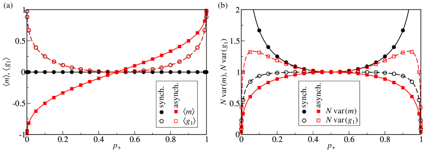
Figure 7: (a) Mean nearest-neighbour correlation $\langle m\rangle$ and second-nearest neighbour correlation $\langle g_{1}\rangle$ in the stochastic voter model. Black curves and symbols are for synchronous, red for asynchronous updates. Analytic predictions (Eq. 122, 124, 126, 128) are shown as solid and dashed curves. The results of Monte Carlo simulations for a chain of length $N=100$ are shown as circles and squares. (b) The same for the variances of $m$ and $g_{1}$ (Eq. 123, 125, 127, 129).

Combining the results above, we can now analytically solve the stochastic synchronous and asynchronous voter models introduced in Sec. 2 and 4. With Eq. 5 we can translate $m$ and $g_{1}$ of the Ising model into correlations between the opinions of nearest and next-nearest neighbours,

$$\langle m\rangle=\frac{1}{N}\left\langle\sum_{i}\omega_{i}\omega_{i+1}\right\rangle,$$ (118)

$$\langle g_{1}\rangle=\frac{1}{N}\left\langle\sum_{i}\omega_{i}\omega_{i+2}\right\rangle,$$ (119)

where the second equation follows from Eq. 63 and $\omega_{i+1}^{2}=1$. The variances of $m$ and $g_{1}$ are proportional to the second partial derivatives of $\ln Z$ with respect to either $x$ or $y$, thus

$$N\mathop{\mathrm{var}}(m)=\frac{\chi}{\beta},$$ (120)

$$N\mathop{\mathrm{var}}(g_{1})=\frac{1}{N}\frac{\partial^{2}}{\partial y^{2}}\ln Z,$$ (121)

where the derivative in the last equation has to be evaluated at $x=0$ for synchronous and $y=0$ for asynchronous updates. For synchronous updates, we have in fact evaluated this derivative already in Eq. 73 because in this case $N\mathop{\mathrm{var}}(g_{1})=C/(k_{B}\beta^{2}J^{2})$. The corresponding calculation for asynchronous updates can be performed by differentiating the partition functions in Eq. 52 and 53.

Inserting Eq. 9 into Eq. 58, 61, 67 and 73, we obtain for the synchronous voter model in the thermodynamic limit

$$\lim_{N\to\infty}\langle m\rangle=\begin{cases}1&\text{if $N$ is odd and either $p_{+}=0$ or $p_{+}=1$},\\ 0&\text{otherwise},\end{cases}$$ (122)

$$\lim_{N\to\infty}[N\mathop{\mathrm{var}}(m)]=\frac{1}{2\sqrt{p_{+}p_{-}}},$$ (123)

$$\lim_{N\to\infty}\langle g_{1}\rangle=\frac{1-2\sqrt{p_{+}p_{-}}}{1+2\sqrt{p_{+}p_{-}}},$$ (124)

$$\lim_{N\to\infty}[N\mathop{\mathrm{var}}(g_{1})]=\frac{8\sqrt{p_{+}p_{-}}}{(1+2\sqrt{p_{+}p_{-}})^{2}},$$ (125)

where, as before, $p_{-}=1-p_{+}$. For asynchronous updates the corresponding results are

$$\lim_{N\to\infty}\langle m\rangle=\frac{\sqrt{p_{+}}-\sqrt{p_{-}}}{\sqrt{p_{+}}+\sqrt{p_{-}}},$$ (126)

$$\lim_{N\to\infty}[N\mathop{\mathrm{var}}(m)]=\frac{4\sqrt{p_{+}p_{-}}}{1+2\sqrt{p_{+}p_{-}}},$$ (127)

$$\lim_{N\to\infty}\langle g_{1}\rangle=\frac{1-2\sqrt{p_{+}p_{-}}}{1+2\sqrt{p_{+}p_{-}}},$$ (128)

$$\lim_{N\to\infty}\left[N\mathop{\mathrm{var}}(g_{1})\right]=\frac{16\sqrt{p_{+}p_{-}}(1-\sqrt{p_{+}p_{-}})}{1+4\sqrt{p_{+}p_{-}}(1+\sqrt{p_{+}p_{-}})}.$$ (129)

We plot Eq. 122–129 in Fig. 7. As a numerical confirmation we include the results of Monte Carlo simulations in the same graphs. The numerical and analytic results are in excellent agreement.

Comparing the synchronous with the asynchronous case, we notice that the thermodynamic limits of the nearest-neighbour correlations $\langle m\rangle$ differ significantly. While for synchronous updates nearest neighbours are typically uncorrelated, asynchronous updates build up non-zero correlations. Interestingly, the mean second-nearest neighbour correlations $\langle g_{1}\rangle$ are identical for both update rules. However, the variances differ between the rules: $\mathop{\mathrm{var}}(m)$ is larger for synchronous updates, whereas $\mathop{\mathrm{var}}(g_{1})$ is larger for asynchronous updates.

It is in principle possible to extend the calculations to correlations between more distant neighbours too. For example, $\left\langle\sum\omega_{i}\omega_{i+3}\right\rangle$ can be obtained by formally introducing a three-spin interaction strength $K$ in the Hamiltonian so that $E(\boldsymbol{\sigma})=-K\sum_{i}\sigma_{i}\sigma_{i+1}\sigma_{i+2}-J\sum_{i}\sigma_{i}\sigma_{i+1}-H\sum\sigma_{i}$. The mean third-nearest neighbour correlation follows from differentiating the partition function $Z$ with respect to $K$ and subsequently setting $K=0$ as well as $H=0$ for synchronous, $J=0$ for asynchronous updates. Unfortunately, the transfer matrix method developed in Sec. 5 does not easily generalize to arbitrary $k$-spin interactions [29], but calculating correlations in the voter model from Ising-like Hamiltonians is an intriguing possibility for future research.

12 Conclusion

We have studied two variants of the one-dimensional Ising model: in the first variant the number of positive spins is constrained to an even number; in the second model this number must be odd. We have motivated both models by mapping them to a model of opinion dynamics with either synchronous or asynchronous updates. If the temperature and magnetic field are held constant, the thermodynamic limits of the even and odd Ising models are the same as the limit of the unconstrained model. However, by simultaneously increasing the chain length and lowering the temperature and magnetic field, we have shown that the scaling functions for the even, odd and unconstrained models differ. The mapping from the Ising model has allowed us to obtain explicit formulae for correlations between nearest and next-nearest neighbours in the voter model.

We can generalize the problem posed in this paper to higher dimensions or complex networks by associating spins with the links and enforce an even number of positive spins on every cycle in the graph. In other words, only balanced signed graphs [30] are permitted. Assigning opinions to the nodes and mapping them to spins on the links as in Eq. 5 will naturally generate such graphs from the voter model. It is a fascinating question how this changes the thermodynamic limits compared to the unconstrained model.

References

[1]
[2]
Ising E, Beitrag zur Theorie des Ferromagnetismus,
1925 Z. Physik31 253–258
[3]
Baxter R J, Exactly solved models in statistical
mechanics, 1982 (London: Academic Press)
[4]
Grosso G and Pastori Parravicini G, Solid state physics,
2000 (San Diego: Academic Press)
[5]
Schneidman E, Berry M J II, Segev R and Bialek W, Weak
pairwise correlations imply strongly correlated network states in
a neural population, 2006 Nature440 1007–1012
[6]
Stauffer D, Social applications of two-dimensional Ising
models, 2008 Am. J. Phys.76 470–473
[7]
Siegert A J F and Vezzetti D J, On the Ising model with
long-range interaction, 1968 J. Math. Phys.9
2173–2193
[8]
Sherrington D and Kirkpatrick S, Solvable model of a
spin-glass, 1975 Phys. Rev. Lett.35 1792–1796
[9]
Ashkin J and Teller E, Statistics of two-dimensional
lattices with four components, 1943 Phys. Rev.64 178–184
[10]
Fernández-Gracia J, Eguíluz V M and San Miguel M,
Timing interactions in social simulations: the voter model,
2013 in Holme P, Saramäki J (eds), Temporal Networks
331-352 (Berlin: Springer, Berlin)
[11]
Skorupa B, Sznajd-Weron K and Topolnicki R, Phase diagram
for a zero-temperature Glauber dynamics under partially
synchronous updates, 2012 Phys. Rev. E86
051113
[12]
Newman M E J and Barkema G T, Monte Carlo methods in
statistical physics, 1999 (Oxford: Oxford University Press)
[13]
Sznajd-Weron K and Krupa S, Inflow versus outflow
zero-temperature dynamics in one dimension, 2006
Phys. Rev. E74 031109
[15]
Nowak M A, Bonhoeffer S and May R, Spatial games and the
maintenance of cooperation, 1994 Proc. Nat. Acad. Sci91 4877–4881
[16]
Fernández Gracia J, Eguíluz V M and San Miguel M, Update
rules and interevent time distributions: Slow ordering versus no
ordering in the voter model, 2011 Phys. Rev. E84 015103(R)
[17]
Varga L, Vukov J and Szabó G, Self-organizing patterns in
an evolutionary rock-paper-scissors game for stochastic
synchronized strategy updates, 2014 Phys. Rev. E90 042920
[18]
Godfray H C J and Hassell M P, Discrete and continuous
insect populations in tropical environments, 1989
J. Anim. Ecol.58 153–174
[19]
Gallegati M, Keen S, Lux T and Ormerod P, Worrying trends in
econophysics, 2006 Physica A370 1–6
[20]
Kramers H A and Wannier G H, Statistics of the
two-dimensional ferromagnet. Part I, 1941 Phys. Rev.60 252–262
[21]
Nelson D R and Fisher M E, Soluble renormalization groups
and scaling fields for low-dimensional Ising systems, 1975
Ann. Phys.91 226–274
[22]
Bruce A D, Probability density functions for collective
coordinates in Ising-like systems, 1981 J. Phys. C:
Solid State Phys.14 3667–3688
[23]
Bruce A D, Universality in the two-dimensional continuous
spin model, 1985 J. Phys. A: Math. Gen.18
L873–L877.
[24]
Zheng B, Generic features of fluctuations in critical
systems, 2003 Phys. Rev. E67 026114
[25]
García-Pelayo R, Distribution of magnetization in the
finite Ising chain, 2009 J. Math. Phys.50
013301
[26]
Antal T, Droz M and Rácz Z, Probability distribution of
magnetization in the one-dimensional Ising model: effects of
boundary conditions, 2004 J. Phys. A: Math. Gen.37 1465–1478
[27]
Feller W, An introduction to probability theory and its
applications, 1950 (New York: Wiley)
[28]
Olver F W J, Bessel functions of integer order, in
Abramowitz M and Stegun I A (eds.), Handbook of mathematical
functions, 9th printing, 1972 (New York: Dover)
[29]
Fan Y, One-dimensional Ising model with -spin
interactions, 2011 Eur. J. Phys32 1643–1650
[30]
Harary F, On the notion of balance of a signed graph, 1953
Michigan Math. J.2 143–146
[31]
Villain J, Spin glass with non-random interactions, 1977
J. Phys. C: Solid State Phys.10 1717–1734