Lateral downflows in sunspot penumbral filaments and their temporal evolution

Abstract

We study the temporal evolution of downflows observed at the lateral edges of penumbral filaments in a sunspot located very close to the disk center. Our analysis is based on a sequence of nearly diffraction-limited scans of the Fe I 617.3 nm line taken with the CRisp Imaging Spectro-Polarimeter at the Swedish 1 m Solar Telescope. We compute Dopplergrams from the observed intensity profiles using line bisectors and filter the resulting velocity maps for subsonic oscillations. Lateral downflows appear everywhere in the center-side penumbra as small, weak patches of redshifts next to or along the edges of blueshifted flow channels. These patches have an intermittent life and undergo mergings and fragmentations quite frequently. The lateral downflows move together with the hosting filaments and react to their shape variations, very much resembling the evolution of granular convection in the quiet Sun. There is a good relation between brightness and velocity in the center-side penumbra, with downflows being darker than upflows on average, which is again reminiscent of quiet Sun convection. These results point to the existence of overturning convection in sunspot penumbrae, with elongated cells forming filaments where the flow is upward but very inclined, and weak lateral downward flows. In general, the circular polarization profiles emerging from the lateral downflows do not show sign reversals, although sometimes we detect three-lobed profiles which are suggestive of opposite magnetic polarities in the pixel.

1. Introduction

The penumbra of sunspots is a magnetized medium where convection is expected to be strongly suppressed (Biermann, 1941; Cowling, 1953). However, we observe it as a relatively bright structure formed by elongated filaments with typical widths of $0\farcs 2$ (e.g., Danielson, 1961a; Sütterlin, 2001). How energy is transported in the penumbra remains a controversial issue. There is consensus that the mechanism responsible for the penumbral brightness involves magnetoconvection, but the details are still poorly understood.

The most conspicuous dynamic phenomenon in sunspots is the Evershed flow (Evershed, 1909)—a radial outflow of gas with speeds of several km s^-1 and large inclinations to the vertical. The Evershed flow is closely related to the filamentary structure of the penumbra (for a review, see Borrero & Ichimoto, 2011). Given its ubiquity and physical properties, it is believed to play a central role in the energy transport of sunspots.

The origin of the Evershed flow has been the subject of intense debate for decades. Some theoretical models explain it as a siphon flow driven by a gas pressure difference between the footpoints of arched flux tubes (Meyer & Schmidt, 1968; Thomas & Weiss, 1992; Montesinos & Thomas, 1997; Thomas et al., 2006). In other models, the Evershed flow is a hot gas confined to magnetic flux tubes that rises to the solar surface by some sort of convection (e.g., Solanki & Montavon, 1993; Jahn & Schmidt, 1994; Schlichenmaier et al., 1998; Schlichenmaier & Solanki, 2003). At the surface the hot gas cools down by radiative losses, heats the surroundings, and sinks again (Schlichenmaier, 2002). This model produces a bright penumbra (Ruiz Cobo & Bellot Rubio, 2008) and is compatible with observations of both penumbral flows and magnetic fields (Borrero & Ichimoto, 2011).

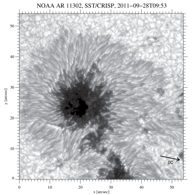
Figure 1.— Continuum intensity image of the main sunspot of AR 11302 as observed through the narrow-band channel of CRISP at an heliocentric angle of 6.8^∘ on 28 September 2011, 09:53 UT. The arrow points to the disk center.

However, the Evershed flow may not be the only manifestation of convection in sunspot penumbrae. Scharmer & Spruit (2006) and Spruit & Scharmer (2006) proposed that penumbral filaments are field-free gaps where regular convection takes place. Such a gappy penumbral model was later revised to include magnetic fields (Scharmer et al., 2008). The velocity field in this model consists of upflows at the center of the filaments and downflows near their edges. Three-dimensional MHD simulations of penumbral fine structure (Heinemann et al., 2007; Rempel et al., 2009a, b; Rempel, 2011, 2012) support this scenario (see the review by Rempel & Schlichenmaier, 2011). According to the simulations, hot gas rising from below the surface is deflected by the inclined magnetic field of the penumbra. This produces a fast flow toward the sunspot border—the Evershed flow. Part of the rising gas turns over laterally and dips down below the solar surface, much in the same way as in quiet Sun granules and intergranular lanes. Thus, the picture favored by the simulations is one of overturning convection. The convective cells are elongated in the preferred direction imposed by the magnetic field (the radial direction), forming penumbral filaments with a fast Evershed outflow along their axes and weaker downflows sideways.

An unambiguous confirmation of this picture—and hence of the convective mechanism operating in the penumbra—requires the detection of lateral downflows at the edges of the filaments. However, the search has proven difficult. Many authors studied the penumbral velocity field without obtaining indications of downward flows near the filament edges (e.g., Mathew et al., 2003; Bellot Rubio et al., 2004; Borrero et al., 2005; Bellot Rubio et al., 2010; Franz & Schlichenmaier, 2009; Ichimoto, 2010; Franz, 2011). Most of those observations were made at intermediate angular resolution, so they might have missed narrow structures. Using higher resolution data acquired with imaging spectrometers, Scharmer et al. (2011) and Joshi et al. (2011) reported the detection of lateral downflows in penumbral filaments. In both cases, a single snapshot of a sunspot at a relatively large distance from the disk center was analyzed. Moreover, the images were strongly deconvolved to bring into view the weakest flow features hidden by stray light arising from turbulence in the Earth’s atmosphere. The need for deconvolution together with the uncertainties in the parameters used to deconvolve the data cast doubts about the reliability of the inferred downflows. After the initial discovery, other studies reported the detection of lateral downflows (Scharmer & Henriques, 2012; Scharmer et al., 2013; Ruiz Cobo & Asensio Ramos, 2013). By now these structures have been observed not only in imaging data, but also in spectropolarimetric measurements from space. In all cases, it has been necessary to account for stray-light contamination or the telescope point-spread function (PSF) to identify them with certainty. For example, Ruiz Cobo & Asensio Ramos (2013) inverted Hinode spectropolarimetric data deconvolved with the telescope PSF, while Tiwari et al. (2013) used a spatially coupled inversion in which the synthetic Stokes profiles were convolved with the Hinode PSF before being compared with the observations. These detections are based on single snapshots too.

Here we study the small-scale velocity field of a sunspot penumbra located close to the disk center, using a very stable time sequence of high resolution spectropolarimetric measurements taken at the Swedish 1 m Solar Telescope (SST; Scharmer et al., 2003a). The observations show weak but ubiquitous lateral downflows at the edges of penumbral filaments. They are visible without performing any deconvolution of the data. For the first time, the temporal evolution of these features is observed and characterized. This allows us to understand why many previous analyses failed to detect them. The spatial and temporal evolution of the small-scale velocity field reveals a convective pattern similar to that prevailing in the quiet Sun, the main difference being the existence of a strong radial Evershed flow.

2. Observations and Data Reduction

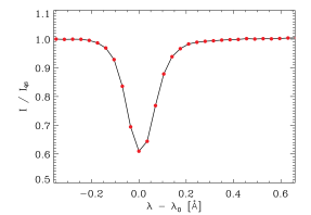
Figure 2.— Mean quiet Sun intensity profile of the Fe I 617.3 nm line in the scan taken at 09:34:00 UT. The spectral sampling is shown with red circles. The $x$-axis represents the calibrated wavelength scale using the umbra as a reference.

The data used here were obtained on 28 September 2011 between 09:20:40 and 10:03:52 UT. We followed the main sunspot of active region AR11302 under excellent seeing conditions (Figure 1). At an heliocentric distance of only 6.8^∘, the spot was located very close to the disk center. Therefore, projection effects are minimized and the line-of-sight (LOS) velocity mostly represents vertical motions.

The observations consist of time sequences of full Stokes measurements in the photospheric Fe I 617.3 nm line. They were acquired with the CRisp Imaging Spectro-Polarimeter (CRISP; Scharmer, 2006) at the SST on La Palma (Spain). CRISP is a dual Fabry-Pérot interferometer capable of delivering nearly diffraction-limited observations with the help of the SST adaptive optics system (Scharmer et al., 2003b) and the Multi-Object, Multi-Frame Blind Deconvolution image restoration technique (MOMFBD; van Noort et al., 2005).

Since we are interested in detecting lateral downflows that may be narrow and weak, our aim was to secure very high spatial resolution observations and high sensitivity to velocities. The diffraction limit of the SST at 617 nm is $\lambda/D=0\farcs 13$, or 90 km on the Sun. On the other hand, we chose the Fe I 617.3 nm line because it is a narrow photospheric transition suitable for Doppler shift measurements, has a clean continuum, and do not show conspicuous line blends or telluric lines nearby.

The Fe I 617.3 nm line was sampled at 30 wavelength positions, covering the range from $-35.0$ to $+66.5$ pm in steps of 3.5 pm (Figure  2). One spectral scan was completed in 32 s. We performed 9 acquisitions per modulation state, obtaining 36 images per wavelength position. The exposure time of the individual images was 17 ms as set by an optical chopper. The full field of view (FOV) of the observations covers an area of $55\arcsec\times 55\arcsec$ with a plate scale of 0$\farcs$059 per pixel.

A very precise data reduction is crucial to this study, to avoid identifying spurious velocities induced by instrumental errors as lateral downflows. With that in mind we used the new CRISPRED pipeline (de la Cruz Rodríguez et al., 2015). Most of the complications involved in the data reduction arise from corrugations in the surface of the CRISP etalons, that could not be made infinitely flat. CRISP is mounted in telecentric configuration very close to one of the focal planes, comparatively optimizing image quality over a collimated configuration (see comments by Scharmer, 2006). In telecentric configuration, however, the corrugations (cavity errors) produce field-dependent random wavelength shifts of the CRISP transmission profile, which effectively displace the observed line profile on a pixel-by-pixel basis.

Current implementations of image reconstruction techniques assume that there is an object that does not change among different realizations of the seeing. Therefore, any intensity fluctuation that is detected is assumed to be produced by atmospheric aberrations. In the presence of a spectral line profile, cavity errors introduce a pattern of intensity fluctuations that are not caused by seeing motions. Without any compensation for these fluctuations, the resulting reconstructed images can contain small-scale artifacts that correlate with the cavity-error map. This problem usually appears when seeing conditions are not great and/or the line profile is very steep.

As an approximate solution, Schnerr et al. (2011) proposed to correct these fluctuations assuming a quiet-Sun spectral profile. This assumption is somewhat valid on granulation observations, but it is not precise enough in sunspots where the strength and width of the profile substantially deviate from quiet-Sun values. Also, the Fe I 617.3 nm line used here is particularly steep and narrow, compared with, e.g., the Fe I 630 nm lines that have been commonly employed in other photospheric studies.

A much more accurate solution to this problem has been given by de la Cruz Rodríguez et al. (2015). They improved the flat-fielding of the data prior to image reconstruction in two ways. First, the quiet-Sun profile that is present in the flats is removed (Schnerr et al., 2011). To compensate for the intensity fluctuations, all the acquisitions corresponding to the same polarization state and same wavelength within a line scan are summed, resulting in a (somewhat) spatially blurred image of the object with dimensionality $(x,y,\lambda)$. Those spectra are used to estimate the imprint of the cavity error in each pixel, by shifting the line profile to the real observed grid. A linear correction is then introduced in each pixel for each wavelength, polarization state, and time step.

Furthermore, de la Cruz Rodríguez et al. (2015) argue that, since the summed images may still contain distortions from the seeing, it is better to compensate only for the high frequencies present in the cavity map, which are associated with the artifacts produced by cavity errors.

This strategy minimizes the intensity variations due to cavity errors, and also allows to estimate the shift of the wavelength scale on a pixel-by-pixel basis, taking into account how the image is changed by the MOMFBD restoration.

The polarimetric calibration was performed for each pixel as described in van Noort & Rouppe van der Voort (2008). Telescope-induced polarization was corrected using a theoretical model of the SST (Selbing, 2010) with updated parameters for the 617 nm spectral range. Residual seeing within each line scan and wavelength was removed following Henriques (2012), so all polarization states were aligned with subpixel accuracy before demodulating the data. Finally, the resulting time series of Stokes images were de-rotated, co-aligned and de-stretched (to compensate for rubber-sheet motions) as described in Shine et al. (1994).

3. Data Analysis

3.1. Determination of LOS Velocities

We construct LOS velocity maps using line bisectors. The bisector is the curve dividing a spectral line into two halves. It is computed by finding the midpoints of horizontal cuts of the line at different intensity levels, from the core (0%) to the continuum (100%). Bisectors allow the depth dependence of the velocity field to be traced in each pixel, as intensity levels close to the continuum sample deeper layers than those near the line core. By mapping a given bisector level across the FOV, we are measuring velocities from a corrugated geometrical surface on the solar atmosphere.

Bisectors are calculated from the observed intensity profiles using linear interpolation, after spectral gradients due to the CRISP prefilter have been removed. In this paper we focus on the bisectors at the 50, 60 and 70% levels, to progressively sample deeper layers of the photosphere in each pixel. The Evershed flow is stronger close to the continuum forming layer (Rimmele, 1995; Westendorp Plaza et al., 2001; Bellot Rubio, 2003, and others), so in principle bisectors at high intensity levels are advantageous to detect the weak signals expected from lateral downflows.

We have removed the 5-minute photospheric oscillations (Leighton et al., 1962) from the velocity maps using a Fourier filter with cut off speeds of 5 km s^-1 (Title et al., 1989; Straus et al., 1992).

3.2. Velocity Calibration

The filtered Dopplergrams were calibrated using the umbra as a velocity reference (Beckers, 1977). To avoid possible molecular blends, we selected all umbral pixels ($I_{\rm c}<0.45I_{\rm QS}$) with Stokes V amplitude asymmetries smaller than 4%. This criterion is met by approximately 60% of the umbral points.

For each Dopplergram in the sequence, the zero point of the velocity scale was taken to be the average Stokes V zero-crossing point of the umbral pixels selected in that frame. The typical standard deviation of the zero-crossing points used to compute the velocity reference is 110 m s^-1. This can be considered the uncertainty of our velocity calibration. The standard deviation of the average Stokes V zero-crossing points in the different line scans is 3 m s^-1.

4. Results

In this Section we investigate the penumbral velocity field on all spatial scales accessible to our observations. We first describe the Evershed flow as seen in the Dopplergrams. Then we summarize the properties of narrow, elongated downflows that occur at the edges of the penumbral filaments. In the third part of this section we show the evolution of a few representative examples of such downflows. Finally, we present a statistical study of their physical properties in the center-side penumbra.

Figure 3 shows one of the Dopplergrams of the temporal sequence and an enlargement of a center-side penumbral region. The Dopplergram corresponds to the 70% bisector level and samples deep layers of the solar atmosphere. The contours outline the inner and outer penumbral boundaries. The black arrow points to the disk center. A movie of the Dopplergram sequence can be found in the electronic Journal.

4.1. Evershed Flow

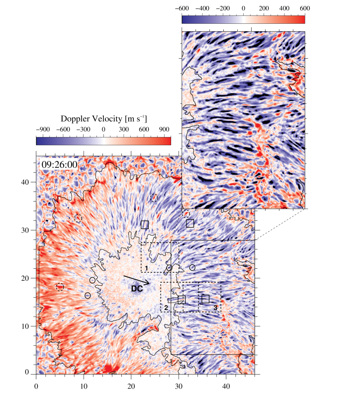
Figure 3.— Velocity field in and around AR 11302 as derived from the line bisectors at the 70% intensity level. Both axes are in arcsec. The arrow points to the solar disk center and contours outline the inner and outer boundaries of the penumbra. Solid circles show examples of penumbral grains, dashed circles mark strong returning Evershed flows, and small squares enclose lateral downflows. The dashed rectangles labeled 1–3 identify the areas used in Figures 6, 7 and 8. A region of the center-side penumbra is enlarged and displayed with a different scale in the right panel to better illustrate the existence of lateral downflows at the edges of penumbral filaments.

Despite the small heliocentric angle of the sunspot, the typical Evershed pattern is clearly seen in Figure 3. The limb-side and center-side penumbrae are redshifted and blueshifted, respectively, indicating motions away from and to the observer. These motions become stronger toward the outer sunspot boundary. The observed pattern of Doppler shifts demonstrates that the penumbral flow is, to first order, a radially directed outflow whose inclination to the vertical steadily increases toward the outer penumbra. This picture does not differ much from previous results (e.g., Stanchfield et al., 1997; Schlichenmaier & Schmidt, 2000; Mathew et al., 2003; Borrero et al., 2004; Bellot Rubio et al., 2004; Rimmele & Marino, 2006). However, the very high spatial resolution of our observations allows us to identify individual flow channels with unprecedented accuracy. Elongated, extremely thin flow structures are observed to stretch radially outward for a few arcseconds in the velocity map. They exhibit opposite velocities on the two sides of the spot. These structures often—but not always—coincide with bright penumbral filaments.

The flow channel heads display conspicuous, localized patches of enhanced blueshifts regardless of their position in the spot, although they are easier to detect in the inner penumbra because that region is less cluttered. The solid circles in Figure 3 mark prominent examples. The strong blueshifts represent upward motions and can be considered to be the sources of the hot Evershed flow. They always occur at the position of bright penumbral grains (Rimmele & Marino, 2006; Ichimoto et al., 2007a). Our observations show them with typical sizes of 0$\farcs$2, in agreement with previous studies.

The tails of the flow channels, especially those near the outer penumbral edge, often display strong redshifts. These patches represent the locations where the Evershed flow returns to the solar surface (e.g., Westendorp Plaza et al., 1997, 2001), now observed with unprecedented clarity as separate structures. They can be identified most easily in the center-side penumbra, thanks to their large contrasts over the blue background. Examples are marked with dashed circles in Figure 3. The downflows occurring in these patches are supersonic and nearly vertical (Bellot Rubio, 2010; van Noort et al., 2013), although the bisector analysis yields modest LOS velocities of order 2 km s^-1.

4.2. Lateral Downflows

In addition to these flow structures, our Dopplergrams reveal the existence of a new flow component producing small patches of weak redshifts in between the flow filaments. They are observed everywhere across the spot, except in the limb-side penumbra where the prevailing redshifts hide them efficiently. By contrast, the patches are very conspicuous in the center-side penumbra and the region perpendicular to the symmetry line (the line connecting the sunspot to the disk center). Examples of such lateral redshifts are indicated in Figure 3 with small squares. Their general properties can be summarized as follows:

• They are associated with flow filaments. Sometimes the lateral redshifts can be observed on both sides of the filament, but most often they appear only on one side.

• Their sizes vary from small roundish patches $\sim$0$\farcs$15 in diameter to elongated, narrow structures flanking the flow filaments for more than 1″.

• In the center-side penumbra, they show bisector velocities ranging from $\sim$100 to $\sim$500 m s^-1 at the 70% intensity level. These flows are therefore much weaker than those observed in the adjacent filaments.

• Their velocities are stronger in deeper photospheric layers. In the center-side penumbra, they exhibit mean maximum velocities of 165, 195 and 210 m s^-1 at the 50, 60 and 70% intensity levels, respectively.

What do these flows represent? The Doppler velocities displayed in Figure 3 are projections of the actual velocity vector to the LOS. Along the symmetry line, only radial and vertical motions can contribute to the LOS velocity. The center-side penumbra near the symmetry line is dominated by the blueshifts produced by the radial Evershed outflow. Any redshift observed there must be due to vertical downdrafts or to inward horizontal motions. The latter can be ruled out because the structures move outward rather than inward (see below). Thus, the lateral redshifts must correspond to downward vertical flows.

In the region perpendicular to the symmetry line, only horizontal flows along the azimuthal direction (i.e., perpendicular to the radial direction of the filaments) and vertical flows can produce non-zero LOS velocities. The global reduction of the LOS velocity observed there is caused by the vanishing contribution of the radial Evershed flow. In that part of the spot, however, we still detect small redshifted patches in between the penumbral filaments. Since they often occur in pairs on either side of the same flow channel, they cannot be due to horizontal motions away from the filament, as those motions would produce velocity patches of opposite sign. In addition, due to the small heliocentric angle of the spot, one would need very large azimuthal flows to explain the observed LOS velocities. Therefore, also in this region we conclude that the redshifted patches represent vertical motions away from the observer, i.e., downflows.

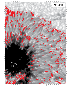
Figure 4.— Spatial distribution of downflows in the penumbra of AR 11302. Red pixels represent locations with bisector velocities larger than 100 m s^-1 at the 70% intensity level, overplotted on the continuum intensity filtergram.

Figure 4 shows the location of the downflows relative to the intensity structures. On top of the continuum intensity filtergram, red pixels indicate bisector velocities larger than 100 m s^-1 at the 70% intensity level. As can be seen, the lateral downflows tend to appear next to penumbral filaments, but sometimes they occur at their edges or even right on them. As a consequence, the lateral downflows are not always associated with dark structures.

Figure 5.— Top row: intensity profiles emerging from a blueshifted flow channel (central panel) and its lateral downflowing regions (right and left panels). The positions of the selected pixels are marked in Figure 8 with plus symbols. Bottom row: line bisectors calculated between the 0 and 80% intensity levels.

Figure 5 displays the intensity profiles emerging from a blueshifted penumbral filament (central panel) and its two lateral downflows (right and left panels). The exact location of the profiles is marked with plus symbols in the close-up of Figure  8. Also depicted are the corresponding line bisectors for intensity levels from 0 to 80%. As can be seen, the intensity profiles emerging from the lateral downflows have slightly darker continua than the flow channel. Other properties such as line widths are similar. The lateral downflows produce bisectors with larger redshifts at higher intensity levels, indicating the existence of velocities that increase with depth in these pixels. The bisector at the position of the flow channel reveals upflows of order 800 m s^-1 that do not change much throughout the atmosphere. These spectral properties reveal the different nature of the central upflows along the filament and the lateral downflows.

4.3. Temporal Evolution of Lateral Downflows

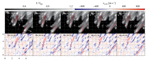
Figure 6.— Temporal evolution of lateral downflows in penumbral filaments located perpendicularly to the symmetry line (case 1). The intensity panels on top have been corrected for a stray light contamination of 40% (see Sect. 5.2). The velocity maps in the second row display the bisector velocities at the 70% intensity level without correction. Red contours outline redshifts greater than 100 m s^-1. The frames are not contiguous in time, as indicated in the upper right corner of each panel. The white arrow plotted in the first intensity panel points to the disk center. Axes are labeled in arcsec.

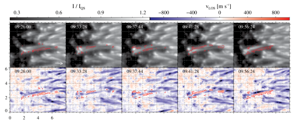
Figure 7.— Example of lateral downflows located at the edges of a conglomerate of filaments protruding into the umbra near the symmetry line (case 2). The layout is the same as in Figure 6.

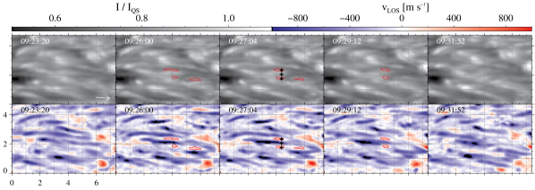
Figure 8.— Lateral downflows at the edges of a filament located in the middle penumbra near the symmetry line (case 3). The layout is the same as in Figure 6. The plus symbols at 09:27:04 UT mark the pixels represented in Figure 5.

We have selected three examples to illustrate the evolution of the lateral downflows (Figures 6,  7, and  8). They are located at different positions across the center-side penumbra (dashed rectangles in Figure 3). Movies covering their entire evolution are available in the electronic Journal.

4.3.1 Case 1

Figure 6 shows a region perpendicular to the symmetry line in the inner penumbra. Two bright filaments protruding into the umbra can be seen in the intensity maps (top row). They appear in the Dopplergrams (bottom row) as two blueshifted flow channels headed by roundish patches that also harbor blueshifts. Since the filaments are nearly perpendicular to the symmetry line, the LOS velocity is the result of azimuthal and vertical motions. Following the arguments of Section 4.1, these blueshifts represent the upward component of the Evershed flow in the penumbra, with velocities of up to 800 m s^-1.

Small redshifted patches can be seen next to the two penumbral filaments. We have identified them with red contours. They never cover the entire length of the filaments, but appear as patchy, more or less elongated structures close to their edges. In the intensity images, they are located next to bright structures or even superposed on them. Sometimes we see the redshifts only on one side of the filament, sometimes on both sides, evolving independently of each other. Given their location, the redshifts are unlikely to be produced by azimuthal motions and must rather be considered as downward motions.

The lateral downflows depicted in Figure 6 are intermittent. Individual patches usually have lifetimes of a few minutes, although the bigger ones are recognizable for up to 10 minutes. Their velocities remain more or less stable with time, but they can split into smaller fragments and/or merge with neighboring patches from one frame to the next. These processes may simply be the result of an inhomogeneous distribution of downward velocities along the filament length, with regions of enhanced flows which are easy to detect and areas of weaker flows that can go largely unnoticed. If the velocities change with time one may get the impression that the patches split and merge, while in reality there exists only one long patch covering the full filament length. An inhomogeneous velocity distribution can also result in apparent drifts of the strongest downflowing patches, as is often observed.

4.3.2 Case 2

Our second example is shown in Figure 7. Now, the filaments are located nearly parallel to the symmetry line and the LOS velocity is mostly due to radial and vertical motions. We see a conglomerate of filaments protruding into the umbra. Small patches of redshifts appear and evolve individually around the most prominent one. Again, these redshifts in the center-side penumbra must be caused by downward motions.

The lateral downflows of Figure 7 are also intermittent, because they appear and disappear with time. They interact between them, merging and splitting in smaller parts as described before. However, the downflowing patches do not evolve in a completely independent way here. In the first frame we observe the blueshifted channel above a bead-like string of lateral downflows of different sizes. The blueshifted region moves downward (in the plane of the paper), interchanging position with the lateral downflows in the second frame. There is a similar transition between the fourth and fifth frames, as the blueshifted filament moves upward and interchanges position with the redshifted patches that are mostly seen again on the other side. Therefore, in this example the lateral downflows appear to follow—or react to—the motion of the flow filament.

4.3.3 Case 3

Our last example corresponds to a mid-penumbral region where the filaments are well aligned with the symmetry line (Figure 8). The Dopplergrams show elongated flow channels harboring blueshifts. These structures are difficult to trace in the continuum images because of their low contrast and the complexity of the region. As in the previous example, the LOS velocity represents the projection of the radial and vertical components of the velocity vector, since the azimuthal component is perpendicular to the LOS. The selected region contains several examples of weak lateral downflows, but we will focus on the ones marked with contours.

Initially, no redshifts can be observed at the edges of the central flow channel. In the second frame, three redshifted regions have appeared. The onset of the redshifts is perhaps triggered by a significant velocity increase happening in the filament, from $-500$ to $-1000$ m s^-1. Two of the patches are located on either side of the filament, approximately at the position of the strongest blueshifts. One of them is more elongated than the other. The third patch is observed near the tail of the filament, but we believe it belongs to a nearby flow channel. The lateral downflows move outward between the second and third frames. By then, their sizes are approximately the same and their velocities have increased from 250 to 400 m s^-1. They no longer flank the strongest blueshifts, which have moved slightly inward. In the fourth frame, the redshifts are further outward, close to the filament tail. Their areas are still similar, but the velocities have decreased back to 250 m s^-1. In the last frame the redshifts have been replaced by blueshifts. This suggest that the development of blueshifts ultimately determines the appearance and visibility of the downflowing patches.

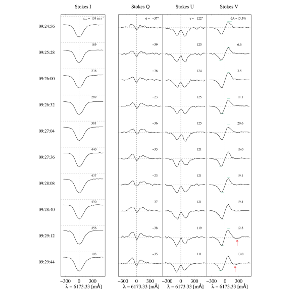
Figure 9.— Temporal evolution of the Stokes profiles emerging from the center of the lowermost lateral downflow in Figure 8. Stokes I, Q, U and V are shown from left to right, and time increases from top to bottom, as indicated on the left hand side. The horizontal lines in the intensity panels represent the continuum of the average quiet Sun profile, making it possible to know if the structure is bright or dark by direct comparison with the observed continuum. The horizontal lines in the other columns indicate zero polarization signal. The small horizontal dashes in the last column represent the amplitudes of the Stokes V profiles. They allow the amplitude asymmetry to be quickly assessed by simple visual inspection. The numbers in the upper right corners of the panels indicate the Doppler velocity at the 70% intensity level (first column), the magnetic field azimuth (second column), the magnetic field inclination (third column; 90^∘ represents fields perpendicular to the LOS and $180^{\circ}$ fields pointing away from the observer along the LOS), and the Stokes V area asymmetry in percent (fourth column). The magnetic parameters have been determined assuming complete Zeeman splitting as in Ortiz et al. (2010).

4.4. Stokes Profiles

In Figure 9 we display the four Stokes profiles emerging from the lowermost lateral downflow marked with a contour in Figure 8, as a function of time. Both linear and circular polarization are clearly seen. The most prominent spectral signature of the profiles, however, is the noticeable asymmetry of Stokes I, which shows increasing redshifts toward the continuum (the vertical lines indicate the rest position of the line).

The linear polarization spectra do not show features worth of mention, except perhaps their amplitude asymmetries. The circular polarization profiles have positive area asymmetries, with the blue lobe being more extended than the red lobe (the exact values are shown next to the Stokes V profiles). In other patches we observe negative area asymmetries. This indicates the existence of velocity gradients along the LOS, possibly coupled with magnetic field gradients, which is consistent with the information provided by the line bisectors. Other than that, the Stokes V profiles emerging from the redshifted patch have the same sign as in the umbra. Thus, the magnetic field vector does not appear to undergo a polarity reversal there. However, toward the end of the sequence, at 09:29:12 and 09:29:44 UT, the Stokes V spectra exhibit a weak third lobe in the red line wing, close to the continuum. This additional lobe (marked with arrows) seems to be strongly redshifted and of opposite polarity compared with the main Stokes V lobes. Similar signals are observed in many pixels of the redshifted patch at those times of the evolution. They occur when the downflowing velocity is decreasing (as seen in the intensity profile), but when the asymmetry of Stokes I is maximum, with a very extended wing toward the red continuum.

Three-lobed profiles have previously been detected in the outer penumbra—both near the sunspot neutral line (Sánchez Almeida & Lites, 1992; Schlichenmaier & Collados, 2002) and far from it (Westendorp Plaza et al., 2001; Bellot Rubio et al., 2002)—, at the position of Evershed flows returning to the solar surface (e.g. Ichimoto et al., 2007a; Franz & Schlichenmaier, 2013), and at the edges of penumbral filaments (Ruiz Cobo & Asensio Ramos, 2013; Scharmer et al., 2013). The mere detection of these profiles indicate the coexistence of fields of opposite polarity along the line of sight. The opposite polarities do not need to be cospatial (i.e., to lie side by side), as they can also be located at different heights in the atmosphere. Whether the third lobe is produced by dragging of the spot field lines by the downflows or by a stable field pointing to the solar surface remains to be investigated.

The direct detection of opposite polarities in the circular polarization spectra may have occurred just by chance, as a result of slightly stronger downflows coupled with more vertical fields leading to a more favorable projection. These fields could be present all the time in the redshifted patches, but without leaving clear signatures in the spectra because of unfavorable conditions. We plan to carry out a full Stokes inversion of the observations to determine whether opposite magnetic polarities exist during the whole lifetime of the patches, or only intermittenly (which would favor dragging and deformation of existing field lines at the edges of penumbral filaments).

4.5. General Properties

We have determined the properties of the lateral downflows through repeated application of the YAFTA feature tracking code (Welsch & Longcope, 2003) to the disk-center penumbral region zoomed in Figure 3, which contains the symmetry line. Lateral downflows are identified as structures with a minimum size of 5 pixels and LOS velocities between 50 m s^-1 and 600 m s^-1 in the individual velocity maps, using the clumping method. The upper limit for the velocity excludes redshifts at the tail of penumbral filaments that correspond to returning Evershed flows. After experimenting with different thresholds, the YAFTA identifications were further refined by retaining only those structures visible in at least four consecutive frames (to avoid false detections due to noise) or coming from the fragmentation of another structure. The features detected through application of these criteria were checked manually to ensure that they represent genuine lateral downflows. All in all, 754 structures (5328 patches) were identified and tracked in the Dopplergram time sequence.

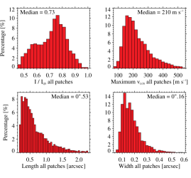
Figure 10.— Histograms of continuum intensity, maximum LOS velocity, length, and width of the redshifted patches observed at the edges of penumbral filaments, considered individually. The median of the distribution is indicated in the upper right corner of the panels.

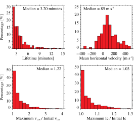
Figure 11.— Histograms of lifetime, mean horizontal speed, ratio of maximum to initial continuum intensity, and ratio of maximum to initial LOS velocity for the lateral downflows, considered as coherent structures that evolve from frame to frame. The median of the distribution is indicated in the upper right corner of the panels.

Figure 10 displays histograms of the continuum intensity, maximum LOS velocity, length, and width of the individual patches detected by YAFTA. The lateral downflows show a broad range of intensities, indicating that they appear both in dark regions outside the filaments and in the bright filament edges. The median value is 0.73 of the quiet Sun continuum intensity. Most patches have a maximum LOS velocity in the range 150–250 m s^-1 with a median of 210 m s^-1. We have fitted an ellipse to each patch to obtain its dimensions. The major axis of the ellipse corresponds to the length of the patch and has a median value of 0$\farcs$53. The width is given by the minor axis, which varies between $\sim$0$\farcs$1 and $\sim$0$\farcs$3 with a median of 0$\farcs$16. Therefore, the redshifted patches tend to be elongated and very narrow.

Figure 11 summarizes the properties of the lateral downflows, considered as coherent structures that can be tracked in subsequent frames of the Dopplergram sequence. We show histograms of lifetimes, horizontal motions, and the ratios of maximum to initial intensities and LOS velocities. For the calculation of the lifetime we have considered only the structures that appear and disappear in situ (i.e., that do not undergo interactions) and those that appear in situ and fragment, but only until their first fragmentation. The fragments are excluded in order not to bias the statistics, since they usually have shorter lifetimes. For this reason it is appropriate to think of the lifetimes as detection times. Most of the lateral downflows can be observed for 4–10 frames. The distribution decreases exponentially, the median being 3.2 minutes (6 frames). Thus, they are short-lived features. This may be intrinsic to the physical mechanism driving the downflows or a consequence of our inability to identify structures when the LOS velocities become too small.

The second panel in Figure 11 shows the distribution of the mean horizontal velocity of the downflowing patches. This parameter has been calculated using well-defined structures for which the direction of motion is clear. Positive (negative) values represent motions away from (to) the umbra. As can be seen, most patches move outward. The median horizontal speed is 85 m s^-1. Finally, the last two panels of the figure show the ratios of maximum to initial mean LOS velocity and continuum intensity. About 75% of the patches develop larger redshifts and brighten during their evolution. The median ratios are 22% and 3%, so the velocity increases more than the brightness.

To study the relation between brightness and LOS velocity we performed an analysis of local fluctuations by subtracting smoothed versions of the continuum intensity filtergrams from the filtergrams themselves. The smoothing was done over 30 pixels, i.e., 1$\farcs$8. The left panel of Figure 12 shows the resulting intensity fluctuations in the region of the center-side penumbra analyzed before. Penumbral filaments are clearly seen as bright structures standing above the mean continuum intensity by some $0.1I_{\rm QS}$. Penumbral grains at the head of the filaments show intensity enhancements that can exceed $0.3I_{\rm QS}$. Between the filaments there are dark lanes with negative variations (around $-0.1I_{\rm QS}$).

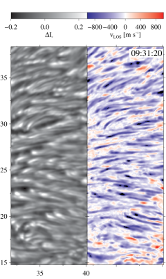
Figure 12.— Continuum intensity fluctuations (left) and bisector velocity at the 70% intensity level (right) in the center-side penumbra of AR 11302. The x- and y-axes indicate the position of the region in Figure 1.

The right panel of Figure 12 displays the corresponding bisector velocities at the 70% intensity level. As can be seen, the blueshifted flow channels are surrounded by regions where the velocities are more shifted to the red. The strongest redshifts however do not always coincide with the darkest areas, as they often occur close to the edges of the filaments.

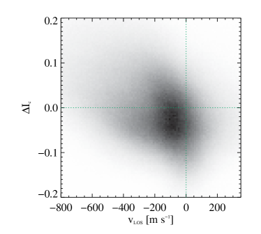
Figure 13.— Scatter plot of continuum intensity fluctuations vs LOS velocity in the center-side penumbral region displayed in Figure 12. The full time sequence is used here.

Figure 13 shows a scatter plot of continuum intensity fluctuations vs LOS velocity for the region displayed in Figure 12. This plot quantifies the behavior described above: pixels with redshifts tend to exhibit negative intensity fluctuations, and vice versa. In fact, the relation is more or less linear, suggesting a correlation between temperatures and flows: the hotter (brighter) structures harbor the largest upflows (blueshifts), whereas the colder structures tend to be ones with the stronger downward velocities (redshifts). This is just the behavior expected from convective flows and has been observed also by Sánchez Almeida et al. (2007) and Scharmer et al. (2011).

5. Discussion

5.1. Why have lateral downflows escaped detection so far?

Sunspot penumbrae have been subject to intense scrutiny for years, using all observational techniques, from monochromatic imaging to Stokes spectropolarimetry, at high and moderate spatial resolution, and high and low cadence. Yet, the lateral downflows studied in this paper have consistently eluded detection (e.g., Jurcák et al., 2007; Borrero et al., 2008; Franz & Schlichenmaier, 2009; Bellot Rubio et al., 2010; Franz, 2011). Having established their properties, we can now provide explanations why their identification was so challenging.

The first problem is our inability to determine the three components of the velocity vector. Only the LOS component is accessible via spectroscopic measurements. Thus, in order to detect vertical motions unambiguously, it is necessary to observe sunspots as close as possible to the disk center, so that the LOS coincides with the normal to the local surface (Bharti et al., 2011). However, this kind of observations are very scarce. Most measurements carried out so far correspond to spots away from the disk center, where the velocity field is dominated by the strong Evershed flow, effectively hiding the weak lateral downflows.

Spectroscopy, and more so spectropolarimetry, is very demanding in terms of exposure time. The long exposures that are required generally mean lower spatial resolution because of stronger seeing degradation, unless the observations are made from space. The highest resolution measurements of sunspot penumbrae using a slit spectrograph were performed by Bellot Rubio et al. (2010) at the SST. Exposure times of 200 ms were needed and, despite the excellent seeing conditions, the achieved spatial resolution was not better than some 0$\farcs$2. This is barely sufficient to detect the largest downflow patches, as the median width of these structures is only 0$\farcs$16. Lateral downflows are also out of reach for the Hinode spectropolarimeter, because of its resolution of about 0$\farcs$32. This may explain why Franz & Schlichenmaier (2009) did not detect them in their careful analysis of sunspots at the disk center.

Of course, fingerprints of such weak downflows must be present in the observed Stokes profiles even at moderate spatial resolution (e.g., the Doppler shifts they produce, their possible opposite polarities, etc) but, being unresolved, separating them from the dominant signals of the strong Evershed flows is not easy—not even for complex Stokes inversions such as those performed by Bellot Rubio (2003), Mathew et al. (2003), Bellot Rubio et al. (2004), Borrero et al. (2005), or Beck (2011). Assuming the penumbra to be a micro-structured magnetic atmosphere, however, Sánchez Almeida (2005) reported downflows and opposite magnetic polarities all across the penumbra from the inversion of spectropolarimetric measurements. These downflows were found to have velocities of up to 10 km s^-1. More recently, hints of the largest downflows patches may have been obtained by Franz & Schlichenmaier (2009, 2013) using the Hinode spectropolarimeter.

The intermittent character of the lateral downflows, which often appear only on one side of the filaments, and for short periods of time (the median lifetime is 3.2 minutes), also imposes strong limitations to slit instruments. The spectroscopic observations of Bellot Rubio et al. (2010), for example, crossed several penumbral filaments, but given the intermittency of the lateral downflows it was unlikely that just a single slit position could catch many instances of them, if any at all. Thus, in retrospect, the chances of success of those observations were low.

The key to detection is probably ultra-high spatial resolution. This is why imaging spectropolarimetric observations provided the first evidence of lateral downflows (Scharmer et al., 2011; Joshi et al., 2011). The measurements were subject to post-facto image restoration to reach the diffraction limit of the SST, which at $\sim$0$\farcs$13 made it possible to resolve the smallest velocity structures ever. Still, corrections other than standard image reconstruction had to be applied to bring out the lateral flows. They were meant to compensate for substantial amounts of stray light, and in practice involved strong deconvolutions of the data. For many observers, such corrections lowered the significance of the discovery.

Reaching ultra-high spatial resolution is not sufficient, however. One needs to subtract from the velocity measurements the oscillation pattern known to affect sunspot penumbrae. This pattern consists of large-scale velocity fluctuations with amplitudes of the order of 100 m s^-1, superposed onto the actual penumbral flow field. Not removing the oscillations may bias the velocities to the point of making some structures appear redshifted when in reality they do not harbor downward motions. Conversely, genuine lateral downflows can be effectively hidden by the oscillations during their blue excursions, since the amplitude of the latter is not much smaller than the LOS velocities of the former.

To subtract the oscillation pattern, one needs to secure time sequences under stable seeing conditions. This is extremely challenging. All imaging spectroscopic measurements presented to date are based on single snapshots and therefore they are affected by oscillations in unknown ways, which casts doubts on the reliability of the reported lateral downflows. To illustrate the importance of this correction, Figure 14 shows typical velocity patterns created by oscillations in our sunspot. They correspond to phases where the center-side penumbra is offset to the blue by an average of $-92$ m s^-1 (top panel) and to the red by 88 m s^-1 (bottom panel). These are the offsets that could not be subtracted in previous investigations because of the lack of temporal information.

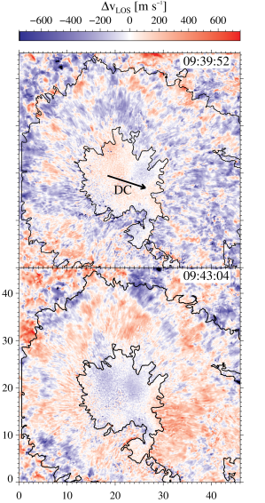
Figure 14.— Amplitudes of the 5-minute oscillation in two frames of our Dopplergram time sequence, corresponding to phases in which the center-side penumbra is offset to the blue by $-92$ m s^-1 (top) and to the red by 88 m s^-1 (bottom). The arrow marks the direction to the disk center.

The choice of spectral line is also relevant, although probably not of prime importance. The discovery paper used the extremely weak C I 538 nm line (Scharmer et al., 2011), which is thought to be one of the deepest-forming lines in the visible but nearly disappears in cool structures like the penumbral background that surrounds the flow channels. In addition, C I 538 nm is affected by molecular blends and cannot be used to set up a reliable velocity reference (Uitenbroek et al., 2012). Joshi et al. (2011) employed the traditional Fe I 630 nm lines, which do not show these problems in the penumbra but have two $O_{2}$ telluric lines distorting their red wings. This is precisely the most important region of the lines for observing downward motions (redshifts), which again may raise doubts on the reliability of the detection. Other lines used in spectroscopic studies include Fe I 709.0 nm. This transition is narrow and therefore very sensitive to velocities (Cabrera Solana et al., 2005), but a CN blend at 709.069 nm distorts its red wing. The Fe I 617.3 nm line we have observed is also very narrow, with the additional advantage of its perfectly flat and clean red continuum. However, it seems to be affected by an Eu II 617.30 nm blend and two other molecular lines in very cold umbrae (Norton et al., 2006).

On top of this all, we have found that a precise correction of subtle instrumental effects is mandatory to unveil the existence of lateral downflows, given the extremely weak Doppler signals they generate. Having imaging spectropolarimetric observations at the diffraction limit and excellent seeing for long periods of time does not help much unless the etalon cavity errors are carefully corrected for. Imperfect corrections produce an orange peel pattern in the velocity maps, with amplitudes that easily exceed those of the lateral downflows themselves. Here we have used the latest version of the CRISP data reduction pipeline, where a new method is implemented to remove the cavity errors. This method produces velocity maps of unprecedented quality and remarkable smoothness.

In summary, the detection of lateral downflows is challenged by a large number of factors that conspire together to hide them in most but the best observations. A good knowledge of their properties, as established here, will hopefully help design new strategies to further study these features and their temporal evolution.

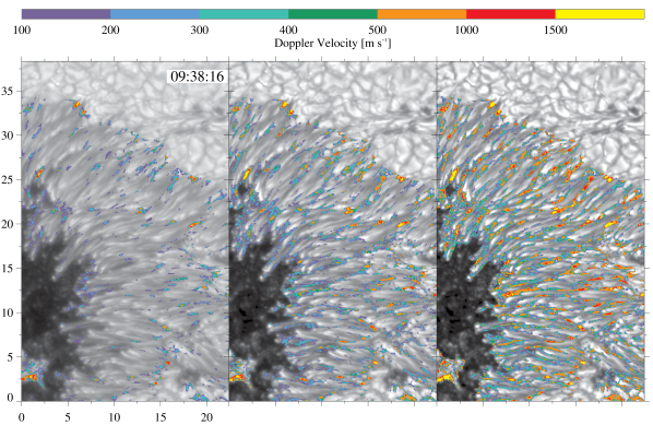
Figure 15.— Comparison of the Doppler velocities to the red resulting from the original and deconvolved data. From left to right: Original observations, compensation for 40% stray light contamination, and compensation for 58% contamination.

5.2. Stray-light Compensated Data

In this section we show the velocities resulting from our observations after deconvolving them with different levels of stray light, to allow direct comparisons with Scharmer et al. (2011); Scharmer et al. (2013) and Scharmer & Henriques (2012). The existence of stray light contamination, its importance, and nature are still a matter of debate (see Löfdahl & Scharmer 2012, Schlichenmaier & Franz 2013, and Scharmer 2014).

We compensate for stray light in the same way as Scharmer et al. (2011). Assuming that $I_{\rm t}$ is the true intensity emerging from a pixel at a given wavelength and polarization state, the observed intensity $I_{\rm o}$ is degraded by stray light as

$$I_{\rm o}=(1-\alpha)I_{\rm t}+\alpha I_{\rm t}\ast P,$$ (1)

where $\alpha$ represents the fraction of stray light contamination and $P$ is a Gaussian PSF with a full width at half maximum $W$. The symbol $\ast$ denotes convolution. Therefore, to obtain the true intensity one needs to deconvolve the original data with some values of $\alpha$ and $W$.

Figure 15 shows the lateral redshifts observed in the original Dopplergrams (left) and in the straylight compensated Dopplergrams, for straylight contaminations of 40% (center) and 58% (right), and FWHM values of $W=1\farcs 8$ and $W=1\farcs 2$, respectively. The velocities correspond to the bisector shifts at the 70% intensity level. They are overplotted on the continuum images resulting from the different deconvolutions.

As expected, the deconvolved continuum images show higher contrasts than the original data. The granulation pattern stands out more prominently as the straylight fraction increases, primarily because the intergranular lanes become darker. Also the penumbral filaments and the outer penumbral border are more clearly defined. In the deconvolved Dopplergrams, umbral dots, penumbral grains, and dark cores of penumbral filaments show higher contrasts than in the original data.

When no stray-light compensation is carried out (left panel in Figure 15), the lateral downflows detected in the center-side penumbra have typical velocities of less than 300 m s^-1. At the tail of penumbral filaments, we see patches with velocities that often exceed 1500 m s^-1 and correspond to Evershed flows returning back to the solar surface. The velocities are always stronger at the center of the patches, for both types of structures. This translates into concentric LOS velocity contours (most easily seen in the case of the final downflows).

The straylight compensated data (center and right panels in Figure 15) show the same redshifted patches, with larger areas and LOS velocities, plus new patches that were not visible originally and show up only after deconvolution. Correcting the data for a straylight contamination of 40% increases the LOS velocities of the lateral downflows by a factor of two on average. Scharmer & Henriques (2012) found a similar behavior. The downflows associated with returning Evershed flows undergo slightly smaller enhancements. As expected, the velocity increase is even stronger in the data compensated for a straylight contamination of 58%, with individual lateral downflows reaching up to 475 m s^-1 compared to the $\sim$150  m s^-1 of the original data.

Our results suggest that the lateral downflows detected by Scharmer et al. (2011), Scharmer & Henriques (2012) and Scharmer et al. (2013) in deconvolved images are probably not mathematical artifacts. Some of those redshifts are actually visible in the original observations, and so they are not created by noise amplification or by the data deconvolution (see the examples in Schlichenmaier & Franz, 2013). We cannot say much about the other structures that show up in the deconvolved images, as they are the result of enhancing inconspicuous signals in the original filtergrams.

5.3. Interpretation

The lateral downflows studied in this paper are compatible with several magnetoconvection modes in sunspot penumbrae. We briefly describe them in the following.

Danielson (1961b) suggested that penumbral filaments represent convective rolls (cells) lying next to each other, with their long dimension being parallel to the horizontal component of the magnetic field. Two of these rolls would form a filament as they turn in opposite directions, creating a bright upflow in the center and two downflows on the external sides of the rolls. This model was ruled out when confronted with observations (see Rempel & Schlichenmaier, 2011). One of the main problems was the lack of evidence for downflows at the filament edges. Our analysis shows them unambiguously, which removes this drawback.

However, lateral downflows may also happen in penumbral flux tubes. Borrero (2007) derived the thermodynamic and magnetic configuration of flux tubes in perfect mechanical equilibrium with the surroundings. He found that flux tubes are stable structures if the magnetic field is mainly aligned with the tube axis and shows a small azimuthal component, i.e., if the field is slightly twisted. In the plane perpendicular to the tube axis, the magnetic field topology resembles two convective rolls through which gas can flow aligned with the magnetic field. The flow would be mainly radial but would show an upward component at the center of the tube and downflows on the sides. Actually, this flow pattern is the one to be expected, since force balance requires the central part of the tube be hotter than the external part, which would naturally trigger convective motions as described above. The model by Borrero (2007) produces penumbral filaments with central dark cores and is consistent with all sunspot magnetic field measurements performed to date.

Finally, the lateral downflows may also be the result of overturning convection in the penumbra, as proposed by Scharmer et al. (2008). According to this model, penumbral filaments are elongated convective cells with two distinct velocity components. Upflows emerge into the surface at the filament head and progressively get more inclined along the filaments until they sink at their tails. At the same time, the upward flows turn over laterally, becoming downdrafts at the filament edges. The resulting convective pattern is very similar to that observed in the quiet Sun, except for the existence of a preferred direction —the one defined by the sunspot magnetic field.

From a pure kinematic point of view, our observations cannot rule out any of these models. Additional criteria need to be invoked to discern between the different scenarios (for example, the existence and spatial distribution of opposite polarities). We note, however, that the mechanism of overturning convection seems to be backed up by the latest 3D numerical simulations (e.g., Rempel et al., 2009a; Rempel, 2011, 2012). Thus, we tentatively give more credence to that scenario, with the caveat that the lateral downflow velocities derived from the data are significantly smaller than those in the simulations ($\sim$210 m s^-1 vs 1 km s^-1). The mismatch persists even when stray light is corrected for.

Independently of the driver of the lateral downflows, the three models predict the existence of a flow connecting them with the central upflows. Such an azimuthal flow (perpendicular to the filament axis) might be responsible for the so-called twisting motions that are seen as dark lanes moving diagonally from the center to the limb side of penumbral filaments (Ichimoto et al., 2007b). Several mechanisms have been proposed to explain these twisting motions (Zakharov et al., 2008; Bharti et al., 2010; Spruit et al., 2010; Bharti et al., 2012). Therefore, the next step to corroborate if they are tracers of the azimuthal component of the velocity field is to study them by spectroscopic means. This analysis could settle the problem of the gas flow in penumbral filaments at photospheric levels.

6. SUMMARY AND CONCLUSIONS

In this paper, we have analyzed the dynamics and temporal evolution of a sunspot penumbra using high-resolution spectropolarimetric measurements in the Fe I 617.3 nm line. The excellent seeing conditions, accurate data reduction, precise wavelength calibration, high temporal cadence and the location of the sunspot very close to the disk center all contribute to make this an unprecedented dataset for sunspot studies.

We report the ubiquitous presence of lateral downflows in penumbral filaments. For the first time, these elusive features are detected without correcting the data for stray light, avoiding the controversies associated with such methods (Schlichenmaier & Franz, 2013). We have removed the undesired imprint of p-modes from the Dopplergrams using Fourier filtering. The resulting velocity maps are less veiled and signals are more stable, as p-modes can make large areas appear completely blueshifted (hiding the lateral downflows) or redshifted (producing artificial downflows). This correction has not been performed previously and it is important.

Lateral downflows appear in our Dopplergrams as elongated redshifted patches surrounding the upflowing penumbral filaments. In the centerside penumbra, they stand out conspicuously over the dominant blueshifts associated with the Evershed flow. By studying examples in different parts of the spot we have been able to rule out radial and azimuthal motions as the cause of the redshifts. We summarize the properties of these structures as follows:

• The downflows are mostly located in dark areas next to penumbral filaments, but some of them occur on the bright filament edges.

• The LOS velocities observed at the $70\%$ bisector level typically range from 150 to 300 m s^-1. Occasionally, stronger downflows exceeding $500$ m s^-1 are detected.

• We find an exponentially decreasing distribution of lifetimes, with nearly all downflows lasting less than 6 minutes. The median lifetime is 3.2 minutes. Within this time span, they can fragment, disappear, and re-appear. They seem to follow the wiggle of the filaments they are associated with. We speculate that forces derived from horizontal pressure balance are somehow responsible for this behavior.

• Lateral downflows show a median length of 0$\farcs$53 and a width of 0$\farcs$16. Therefore, high spatial resolution is needed to detect them.

• In the inner and middle penumbra, the downflowing patches move outward with a median horizontal velocity of 85 m s^-1, whereas bright penumbral grains move inward (Muller, 1973; Sobotka & Sütterlin, 2001; Rimmele & Marino, 2006, and others). The outward horizontal motion decreases the LOS velocity observed in the lateral downflows, so the actual flow speeds could be larger than those indicated by Doppler measurements.

• The lateral downflows detected in the original Doppler maps are found at the same locations in straylight-compensated data, but with enhanced speeds. Thus, our results suggest that at least some of the downflows seen in data corrected for stray light are not mathematical artifacts.

We have compared the continuum intensity fluctuations and the corresponding LOS velocities in the center-side penumbra. Similarly to Sánchez Almeida et al. (2007) and Scharmer et al. (2011), we find that blueshifted areas are generally bright and redshifted areas tend to be darker. These two quantities seem to follow a linear relation, consistent with the operation of some kind of magnetoconvection in the penumbra.

As other authors, we observe upflows along penumbral filaments and downflows at their tails. The upflows return to the solar surface also at the edges of the filaments, producing lateral downdrafts. This supports the existence of overturning convection in the penumbra (Scharmer & Spruit, 2006; Scharmer et al., 2008). The detection of the lateral downflows has been challenging because they are very weak and small. We suggest a scenario where the lateral downflows are produced by elongated convection: adjacent convective cells (filaments) have a predominantly outward flow that returns to the solar surface at their tails, while overturning convection is found along the edges of the filaments. There, matter from neighboring cells is strongly squeezed and allowed to fall down.

Sánchez Almeida (2005) was the first to infer the existence of downflows all over the penumbra from the inversion of moderate resolution spectropolarimetric data. However, it is not clear to us that those downflows and ours represent the same phenomenon, given their very different spatial scales (optically thin versus optically thick) and speeds (tens of km s^-1 versus a few hundred m s^-1).

The velocities we observe in the downflows are significantly smaller than those resulting from the simulations, even after correcting the data for stray light. For this reason, the association of lateral downflows with overturning convection is still not completely unambiguous. In fact, other theoretical scenarios, such as the convective rolls proposed by Danielson (1961b) or the twisted horizontal magnetic flux tubes of Borrero (2007), are also compatible with our observations from a pure kinematical point of view. Distinguishing between them requires a thorough analysis of the vector magnetic field in penumbral filaments and a comparison with the velocity field at similar spatial scales.

References

- Bharti et al. (2011) Bharti, L., Schüssler, M., & Rempel, M. 2011, ApJ, 739, 35
- Bharti et al. (2012) Bharti, L., Cameron, R. H., Rempel, M., Hirzberger, J., & Solanki, S. K. 2012, ApJ, 752, 128
- Bharti et al. (2010) Bharti, L., Solanki, S. K., & Hirzberger, J. 2010, ApJL, 722, L194
- Beck (2011) Beck, C. 2011, A&A, 525, A133
- Bellot Rubio (2003) Bellot Rubio, L. R. 2003, in ASP Conf. Ser. 307, Solar Polarization 3, ed. J. Trujillo Bueno & J. Sánchez Almeida (San Francisco: Astronomical Society of the Pacific), 307
- Bellot Rubio (2010) Bellot Rubio, L. R. 2010, in Astrophysics and Space Science Proceedings, Magnetic Coupling between the Interior and the Atmosphere of the Sun, ed. S. S. Hassan & R. Rutten (Berlin: Springer), 193
- Bellot Rubio et al. (2003) Bellot Rubio, L. R., Balthasar, H., Collados, M., & Schlichenmaier, R. 2003, A&A, 403, L47
- Bellot Rubio et al. (2004) Bellot Rubio, L. R., Balthasar, H., & Collados, M. 2004, A&A, 427, 319
- Bellot Rubio et al. (2002) Bellot Rubio, L. R., Collados, M., Ruiz Cobo, B., & Rodríguez Hidalgo, I. 2002, Nuovo Cimento C, 25, 543
- Bellot Rubio et al. (2010) Bellot Rubio, L. R., Schlichenmaier, R., & Langhans, K. 2010, ApJ, 725, 11
- Beckers (1977) Beckers, J. M. 1977, ApJ, 213, 900
- Biermann (1941) Biermann, L. 1941, VAG, 76, 194
- Borrero (2007) Borrero, J. M. 2007, A&A, 471, 967
- Borrero et al. (2005) Borrero, J. M., Lagg, A., Solanki, S. K., & Collados, M. 2005, A&A, 436, 333
- Borrero et al. (2008) Borrero, J. M., Lites, B. W., & Solanki, S. K. 2008, A&A, 481, L13
- Borrero & Solanki (2010) Borrero, J. M., & Solanki, S. K. 2010, ApJ, 709, 349
- Borrero et al. (2004) Borrero, J. M., Solanki, S. K., Bellot Rubio, L. R., Lagg, A., & Mathew, S. K. 2004, A&A, 422, 1093
- Borrero & Ichimoto (2011) Borrero, J. M., & Ichimoto, K. 2011, LRSP, 8, 4
- Cabrera Solana et al. (2005) Cabrera Solana, D., Bellot Rubio, L. R., & del Toro Iniesta, J. C. 2005, A&A, 439, 687
- Cowling (1953) Cowling, T. G. 1953, in The Solar System, Vol 1: The Sun, ed. G. P. Kuiper (Chicago: University of Chicago Press), 532
- Danielson (1961a) Danielson, R. E. 1961a, ApJ, 134, 275
- Danielson (1961b) Danielson, R. E. 1961b, ApJ, 134, 289
- de la Cruz Rodríguez et al. (2015) de la Cruz Rodríguez, J., Löfdahl, M. G., Sütterlin, P., Hillberg, T., & Rouppe van der Voort, L. 2015, A&A, 573, AA40
- Evershed (1909) Evershed, J. 1909, MNRAS, 69, 454
- Franz (2011) Franz, M. 2011, Ph.D. Thesis, Albert-Ludwigs-Universität Freiburg, Germany
- Franz & Schlichenmaier (2009) Franz, M., & Schlichenmaier, R. 2009, A&A, 508, 1453
- Franz & Schlichenmaier (2013) Franz, M., & Schlichenmaier, R. 2013, A&A, 550, A97
- Heinemann et al. (2007) Heinemann, T., Nordlund, Å., Scharmer, G. B., & Spruit, H. C. 2007, ApJ, 669, 1390
- Henriques (2012) Henriques, V. M. J. 2012, A&A, 548, A114
- Ichimoto (2010) Ichimoto, K. 2010, in Magnetic Coupling between the Interior and the Atmosphere of the Sun, ed. S. S. Hassan & R. Rutten, ASSP, Berlin: Springer-Verlag, 186
- Ichimoto et al. (2007a) Ichimoto, K., Shine, R. A., Lites, B., et al. 2007a, PASJ, 59, 593
- Ichimoto et al. (2007b) Ichimoto,K., & Suematsu, Y., & Tsuneta, S., et al. 2007b, Sci, 318, 1597-1599
- Jahn & Schmidt (1994) Jahn, K., & Schmidt, H. U. 1994, A&A, 290, 295
- Joshi et al. (2011) Joshi, J., Pietarila, A., Hirzberger, J., et al. 2011, ApJL, 734, L18
- Jurcák et al. (2007) Jurcák, J., Bellot Rubio, L., Ichimoto, K., et al. 2007, PASJ, 59, 601
- Leighton et al. (1962) Leighton, R. B., Noyes, R. W., & Simon, G. W. 1962, ApJ, 135, 474
- Löfdahl & Scharmer (2012) Löfdahl, M. G., & Scharmer, G. B. 2012, A&A, 537, A80
- Mathew et al. (2003) Mathew, S. K., Lagg, A., Solanki, S. K., et al. 2003, A&A, 410, 695
- Meyer & Schmidt (1968) Meyer, F., & Schmidt, H. U. 1968, AJS, 73, 71
- Montesinos & Thomas (1997) Montesinos, B., & Thomas, J. H. 1997, Natur, 390, 485
- Ortiz et al. (2010) Ortiz, A., Bellot Rubio, L. R., & Rouppe van der Voort, L. 2010, ApJ, 713, 1282
- Muller (1973) Muller, R. 1973, SoPh, 29, 55
- Norton et al. (2006) Norton, A. A., Graham, J. P., Ulrich, R. K., et al. 2006, SoPh, 239, 69
- Rempel et al. (2009a) Rempel, M., Schüssler, M., & Knölker, M. 2009a, ApJ, 691, 640
- Rempel et al. (2009b) Rempel, M., Schüssler, M., Cameron, R. H., & Knölker, M. 2009b, Sci, 325, 171
- Rempel (2011) Rempel, M. 2011, ApJ, 729, 5
- Rempel (2012) Rempel, M. 2012, ApJ, 750, 62
- Rempel & Schlichenmaier (2011) Rempel, M., & Schlichenmaier, R. 2011, LRSP, 8, 3
- Rimmele (1995) Rimmele, T. R. 1995, A&A, 298, 260
- Rimmele & Marino (2006) Rimmele, T., & Marino, J. 2006, ApJ, 646, 593
- Ruiz Cobo & Asensio Ramos (2013) Ruiz Cobo, B., & Asensio Ramos, A. 2013, A&A, 549, L4
- Ruiz Cobo & Bellot Rubio (2008) Ruiz Cobo, B., & Bellot Rubio, L. R. 2008, A&A, 488, 749
- Sánchez Almeida & Lites (1992) Sánchez Almeida, J., & Lites, B. W. 1992, ApJ, 398, 359
- Sánchez Almeida (2005) Sánchez Almeida, J. 2005, ApJ, 622, 1292
- Sánchez Almeida et al. (2007) Sánchez Almeida, J., Márquez, I., Bonet, J. A., & Domínguez Cerdeña, I. 2007, ApJ, 658, 1357
- Selbing (2010) Selbing, J. 2010, arXiv:1010.4142
- Scharmer (2006) Scharmer, G. B. 2006, A&A, 447, 1111
- Scharmer (2014) Scharmer, G. B. 2014, A&A, 561, A31
- Scharmer et al. (2003a) Scharmer, G. B., Bjelksjo, K., Korhonen, T. K., Lindberg, B., & Petterson, B. 2003a, Proc. SPIE, 4853, 341
- Scharmer et al. (2003b) Scharmer, G. B., Dettori, P. M., Löfdahl, M. G., & Shand, M. 2003b, Proc. SPIE, 4853, 370
- Scharmer et al. (2013) Scharmer, G. B., de la Cruz Rodriguez, J., Sütterlin, P., & Henriques, V. M. J. 2013, A&A, 553, A63
- Scharmer & Henriques (2012) Scharmer, G. B., & Henriques, V. M. J. 2012, A&A, 540, A19
- Scharmer et al. (2011) Scharmer, G. B., Henriques, V. M. J., Kiselman, D., & de la Cruz Rodríguez, J. 2011, Sci, 333, 316
- Scharmer et al. (2008) Scharmer, G. B., Nordlund, Å., & Heinemann, T. 2008, ApJL, 677, L149
- Scharmer & Spruit (2006) Scharmer, G. B., & Spruit, H. C. 2006, A&A, 460, 605
- Schlichenmaier et al. (1998) Schlichenmaier, R., Jahn, K., & Schmidt, H. U. 1998, A&A, 337, 897
- Schlichenmaier (2002) Schlichenmaier, R. 2002, AN, 323, 303
- Schlichenmaier & Collados (2002) Schlichenmaier, R., & Collados, M. 2002, A&A, 381, 668
- Schlichenmaier & Franz (2013) Schlichenmaier, R., & Franz, M. 2013, A&A, 555, A84
- Schlichenmaier & Schmidt (2000) Schlichenmaier, R., & Schmidt, W. 2000, A&A, 358, 1122
- Schlichenmaier & Solanki (2003) Schlichenmaier, R., & Solanki, S. K. 2003, A&A, 411, 257
- Schnerr et al. (2011) Schnerr, R. S., de La Cruz Rodríguez, J., & van Noort, M. 2011, A&A, 534, A45
- Shine et al. (1994) Shine, R. A., Title, A. M., Tarbell, T. D., et al. 1994, ApJ, 430, 413
- Sobotka & Sütterlin (2001) Sobotka, M., & Sütterlin, P. 2001, A&A, 380, 714
- Solanki & Montavon (1993) Solanki, S. K., & Montavon, C. A. P. 1993, A&A, 275, 283
- Spruit & Scharmer (2006) Spruit, H. C., & Scharmer, G. B. 2006, A&A, 447, 343
- Spruit et al. (2010) Spruit, H. C., Scharmer, G. B., Löfdahl, M. G. 2010, A&A, 521, A72
- Stanchfield et al. (1997) Stanchfield, D. C. H., II, Thomas, J. H., & Lites, B. W. 1997, ApJ, 477, 485
- Straus et al. (1992) Straus, T., Deubner, F.-L., & Fleck, B. 1992, A&A, 256, 652
- Sütterlin (2001) Sütterlin, P. 2001, A&A, 374, L21
- Title et al. (1989) Title, A. M., Tarbell, T. D., Topka, K. P., et al. 1989, ApJ, 336, 475
- Tiwari et al. (2013) Tiwari, S. K., van Noort, M., Lagg, A., & Solanki, S. K. 2013, A&A, 557, A25
- Thomas & Weiss (1992) Thomas, J. H., & Weiss, N. O. 1992, in Sunspots: Theory and Observations, ed. J. H. Thomas & N. O. Weiss, NATO ASI Series C375
- Thomas et al. (2006) Thomas, J. H., Weiss, N. O., Tobias, S. M., & Brummell, N. H. 2006, A&A, 452, 1089
- Uitenbroek et al. (2012) Uitenbroek, H., Dumont, N., & Tritschler, A. 2012, in ASP Conf. Ser. 463, Second ATST-EAST Meeting: Magnetic Fields from the Photosphere to the Corona, ed. T. R. Rimmele et al. (San Francisco: Astronomical Society of the Pacific), 99
- van Noort et al. (2005) van Noort, M., Rouppe van der Voort, L., & Löfdahl, M. G. 2005, SoPh, 228, 191
- van Noort & Rouppe van der Voort (2008) van Noort, M. J., & Rouppe van der Voort, L. H. M. 2008, A&A, 489, 429
- van Noort et al. (2013) van Noort, M., Lagg, A., Tiwari, S. K., & Solanki, S. K. 2013, A&A, 557, A24
- Welsch & Longcope (2003) Welsch, B. T., & Longcope, D. W. 2003, ApJ, 588, 620
- Westendorp Plaza et al. (1997) Westendorp Plaza, C., del Toro Iniesta, J. C., Ruiz Cobo, B., et al. 1997, Natur, 389, 47
- Westendorp Plaza et al. (2001) Westendorp Plaza, C., del Toro Iniesta, J. C., Ruiz Cobo, B., & Martínez Pillet, V. 2001, ApJ, 547, 1148
- Zakharov et al. (2008) Zakharov, V., Hirzberger, J., Riethmüller, T. L., Solanki, S. K., & Kobel, P. 2008, A&A, 488, L17