Blazar Variability and Evolution in the GeV Regime

Abstract

One of the most important problem of the blazar astrophysics is to understand the physical origin of the blazar sequence. In this study, we focus on the GeV gamma-ray variability of blazars and evolution perspective we search the relation between the redshift and the variability amplitude of blazars for each blazar subclass. We analyzed the Fermi-LAT data of the TeV blazars and the bright AGNs (flux $\geq$ 4$\times 10^{-9}$ cm^-2s^-1) selected from the 2LAC (the 2nd LAT AGN catalog) data base. As a result, we found a hint of the correlation between the redshift and the variability amplitude in the FSRQs. Furthermore the BL Lacs which have relatively lower peak frequency of the synchrotron radiation and relatively lower redshift, have a tendency to have a smaller variability amplitude.

I Introduction

The blazar is the class of the active galactic nuclei (AGN) which has the most number of extragalactic source in the very-high-energy gamma-ray regime ($E>100$ GeV)TeVCat . They are characterized by double-peaked nonthermal emission with spectral energy distribution (SED) in radio to gamma-ray regime. Blazars include BL Lacertae objects (BL Lacs) and flat spectrum radio quasars (FSRQs). In addition BL Lacs include high-frequency peaked BL Lac objects (HBLs), intermediate-frequency peaked BL Lac objects (IBLs) and low-frequency peaked BL Lac objects (LBLs). In the leptonic model, the low and high bump of SED is explained by the synchrotron and the Synchrotron Self Compton (SSC) and/or External Compton (EC) radiations. The estimation of EC in the second hump is a matter of great importance in estimating external photons.

One of the characteristic of the blazar spectra is blazar sequence. In 1998, Fossati et al. combined three complete blazar samplesFossati1998 ; The 2 Jy samples of FSRQsPadovani1992 , the radio selected 1 Jy samples of BL LacsKuhr1981 and the X-ray selected sample(Einstein Slew Survey) of BL Lacs Elvis1992 . The thirty-third sources of selected sample were detected in high-energy gamma-ray regime ($E>100$ MeV) by the EGRET instrument on-board the compton gamma ray observatory (CGRO). These sources were devided 5 bins based on the 5 GHz radio luminosity and averaged the SED of the each type of the blazars. The made SED suggested some relationship; first, the synchrotron peak frequency and the bolometric luminosity have the anti-correlation. second, the synchrotron peak frequency and the compton peak frequency have the positive-correlation. finally, the compton dominance (the ratio of the inverse Compton to synchrotron luminosity) and the bolometric luminosity have positive-correlation. These correlations are known as “the blazar sequence” in considering the blazar physics. We aim to reveal the relation between the evolution process of AGNs and the blazar sequence based on the systematical study for many blazars .

In this study, we calculated $\sim 100$ AGNs (blazars) to find the difference of the variability amplitude in blazar types and evolution of the variability amplitude (activity). We applied the fractional variability amplitude ($F_{\rm var}$) to calculate the variability amplitude considering the error. The $F_{\rm var}$ is defined as Eq.(1) which was given by Vaughan et al. (2003).

$$F_{\rm var}=\sqrt{\frac{S^{2}-\overline{\sigma_{err}^{2}}}{\overline{F}^{2}}}$$ (1)

Note that $S^{2}$ is the total variance of the light curve, $\overline{\sigma_{err}^{2}}$ is the mean square of flux error and $\overline{F}^{2}$ is the square of mean flux. Fvar error (uncertainty) is defined as Eq.(2) by Poutanen et al. (2008).

$$\Delta F_{\rm var}=\sqrt{F_{\rm var}^{2}+err({\sigma_{{\rm{\tiny{NXS}}}}^{2}})}-F_{\rm var}$$ (2)

Where $err({\sigma_{{\rm{\tiny{NXS}}}}^{2}})$ is defined as Eq.(3) by Vaughan et al. (2003)

$$err({\sigma_{{\rm{\tiny{NXS}}}}^{2}})=\sqrt{{\left(\sqrt{\frac{2}{N}}\frac{\overline{\sigma_{err}^{2}}}{F^{2}}\right)}^{2}+{\left(\sqrt{\frac{\overline{\sigma_{err}^{2}}}{N}}\frac{2F_{\rm var}}{F}\right)}^{2}}$$ (3)

$F_{\rm var}$ is often used in computation variability amplitude for each spectral bandMAGIC2014 .

In this study, we studied the flux variation of AGNs with the $F_{\rm var}$ on the high-energy gamma-ray regime to get the variation charactor of each class (type).

II DATA SELECTION

Table 1: Analyzed AGN list 2LAC ; TeVCat

Source	Redshift	Class	Source	Redshift	Class	Source	Redshift	Class
name	z	(type)	name	z	(type)	name	z	(type)
Messier 87	0.0044	FRI	MS 1221.8+2452	0.218	HBL	4C +55.17	0.899298	FSRQ
NGC 1275	0.017559	FRI	PKS 0301-243	0.26	HBL	PKS 0823-223	0.91	IBL
Mrk 421	0.031	HBL	S2 0109+22	0.265	IBL	PKS 0420-01	0.916	FSRQ
Mrk 501	0.034	HBL	1ES 0414+009	0.287	HBL	AO 0235+164	0.94	LBL
1ES 2344+514	0.044	HBL	S5 0716+714	0.31	IBL	S3 0218+357	0.944	Blazar
Mrk 180	0.045	HBL	OT 081	0.322	LBL	OP 313	0.997249	FSRQ
1ES 1959+650	0.048	HBL	1ES 0502+675	0.341	HBL	PKS 0454-234	1.003	FSRQ
AP Lib	0.049	LBL	PKS 1510-089	0.361	FSRQ	4C +14.23	1.038	FSRQ
1ES 1727+502	0.055	HBL	3C 66A	0.41	IBL	PKS 2201+171	1.076	FSRQ
BL Lacertae	0.069	IBL	PKS 0735+17	0.424	LBL	PKS 0426-380	1.111	LBL
PKS 2005-489	0.071	HBL	4C +21.35	0.432	FSRQ	PKS B1908-201	1.119	FSRQ
RGB J0152+017	0.08	HBL	1ES 0647+250	0.45	HBL	OG 050	1.254	FSRQ
1ES 1741+196	0.083	HBL	PG 1553+113	0.5	HBL	PKS 1551+130	1.30814	FSRQ
W Comae	0.102	IBL	GB 1310+487	0.501	FSRQ	PKS 0244-470	1.385	FSRQ
1ES 1312-423	0.105	HBL	PKS 2326-502	0.518	FSRQ	PKS 2023-07	1.388	FSRQ
VER J0521+211	0.108	IBL	3C 279	0.536	FSRQ	S4 1030+61	1.40095	FSRQ
PKS 2155-304	0.116	HBL	MG2 J071354+1934	0.54	FSRQ	PKS 0402-362	1.417	FSRQ
B3 2247+381	0.1187	HBL	BZQ J0850-1213	0.566	FSRQ	PKS 0250-225	1.419	FSRQ
RGB J0710+591	0.125	HBL	PKS 1424+240	0.6035	IBL	PKS 1454-354	1.424	FSRQ
H 1426+428	0.129	HBL	4C 31.03	0.603	FSRQ	B2 1520+31	1.484	FSRQ
1ES 1215+303	0.13	HBL	PMN J2345-1555	0.621	FSRQ	PKS 2052-47	1.489	FSRQ
PKS 1717+177	0.137	LBL	PKS 1244-255	0.633	FSRQ	PKS 2227-08	1.55999	FSRQ
1ES 0806+524	0.138	HBL	S4 1849+67	0.657	FSRQ	TXS 1013+054	1.7137	FSRQ
1ES 0229+200	0.14	HBL	4C +56.27	0.664	LBL	PKS 0215+015	1.721	FSRQ
1RXS J101015.9-311909	0.142639	HBL	S5 1803+784	0.68	LBL	MG1 J123931+0443	1.76095	FSRQ
TXS 1055+567	0.14333	IBL	Ton 599	0.724565	FSRQ	MG2 J101241+2439	1.805	FSRQ
3C 273	0.158	FSRQ	B2 0716+33	0.779	FSRQ	4C +38.41	1.81313	FSRQ
H 2356-309	0.165	HBL	TXS 0106+612	0.785	FSRQ	PKS 0805-07	1.837	FSRQ
PKS 0829+046	0.173777	LBL	PKS 1622-253	0.786	FSRQ	PKS 1502+106	1.83928	FSRQ
1ES 1218+304	0.182	HBL	B2 2234+28A	0.795	LBL	4C 01+02	2.099	FSRQ
1ES 1101-232	0.186	HBL	PKS 0440-00	0.844	FSRQ	PKS 1329-049	2.15	FSRQ
1ES 0347-121	0.188	HBL	OC 457	0.859	FSRQ	S4 0917+44	2.18879	FSRQ
RBS 0413	0.19	HBL	3C 454.3	0.859	FSRQ	PMN J1344-1723	2.506	FSRQ
OX 169	0.211	FSRQ	TXS 1920-211	0.874	FSRQ
1ES 1011+496	0.212	HBL	PKS 0537-441	0.892	LBL

We selected AGNs from the second LAT AGN catalog (2LAC)2LAC and TeVCatTeVCat . Selection criteria were as follows,

1. : It was decided which subclass was belonged to (HBL or IBL or LBL or FSRQ).

2. : It had known redshift.

3. : flux $\geq 4\times 10^{-9}$ cm^-2 s^-1 in 2LAC.

Table 1 shows the analyzed AGN list which 102 sources are included in. Source name, redshift, and class(type) are cited from 2LAC and TeVCat.

The redshift of PKS 1424+240 was referred to Furniss(2013)Furniss2013 . According to the TeVCatTeVCat , the blazar class of S3 0218+357 (z=0.944) was not determined but we used it as high redshift VHE gamma-ray emitter.

III DATA ANALYSIS

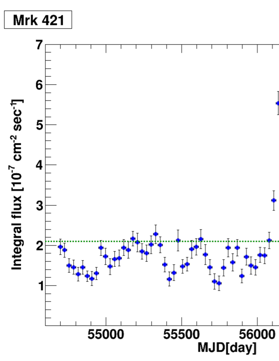
Figure 1: Examples of the gamma-ray light curve about 6 years in 0.1–300 GeV. Blue plots: data points with a bin size of 30 days (bin size of last it is only about 4.4 days). Red allows: 95% C.L. upper limits. Green dotted lines: average flux of whole period. Left panel: Mrk 421(HBL). Right panel: PKS 0454-234(FSRQ).

We analysed the Fermi reprocessed pass 7 data between 2008 August 04 and 2014 June 09, using the unbinned likelihood analysis with the Fermi Science Tools package version v9r33p0 available from the Fermi Science Support Center (FSSC)FSSC . The likelihood analysis was selected that the events with photon energies in the range of 0.1-300 GeV and a Region Of Interest (ROI) of 10 degrees centered at the position of Table 1 sources. We used “SOURCE” class (“evclass = 2”) including both front and back events, because the “SOURCE” class is recommended for off-plane point source analysis by the likelihood analysis Anarecom . We excluded events with zenith angles larger than 100 degrees and time intervals when the rocking angle was larger than 52 degrees. The set of the instrument response functions of “P7REP_SOURCE_V15” was applied. Models which were used in this study include the isotropic diffuse background (iso_source_v05.txtFSSCBG ), galactic diffuse background (gll_iem_v05_rev1.fitFSSCBG ) and the Second Fermi LAT Catalog (2FGL) sources in ROI of 10 degrees centered at the position of Table 1 sources. The spectrum model was according to the 2FGL. Target blazars (Table 1) were fitted with a Log-Parabola (LP):

$$\frac{dN}{dE}=N_{0}\left(\frac{\rm E}{{\rm E}_{0}}\right)^{-(\alpha+\beta{\rm log}({\rm E}/{\rm E}_{0}))}$$ (4)

because LP is typically used for modeling blazar spectraFermiSpectra . Where $N_{0}$[cm^-2 s^-1 MeV^-1] is normalization parameter, E₀ [MeV] is scale parameter, $-(\alpha+\beta{\rm log}({\rm E}/{\rm E}_{0}))$ is spectrum index. If the parameter $\beta$ is zero, LP is equal to Powar-Law spectrum. In this paper we fixed E₀ parameter of targets to E₀ = 100 MeV.

We judged the flux variation of target sources by some steps.
Step I: gamma-ray light curves, which width of the time bins was fixed on 30 days (shortest bin in this study), was made.
Step II: if calculated $F_{\rm var}$ was not required “Selection Criteria”, we adopted more large bin size (60 days, 90 days, 150 days, and 300 days).
“Selection Criteria” were as follows, I. More than 40 % of the calculated integral flux of each bin were detected. II. Significant (over 2$\sigma$) variation was detected by the $\chi^{2}$ test in the analyzed period. If the selection criteria I. and II. cleared, $F_{\rm var}$ of the target could be calculated.

IV RESULTS and DISCUSSION

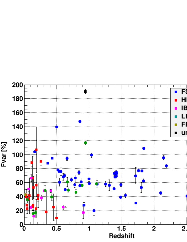
Figure 2: The $F_{\rm var}$ as a function of the redshift. Square and circle marks indicate TeVCat and not TeVCat sources, respectively. Each subclass of blazars are plotted in different colors (Blue:FSRQ, Red: HBL, Magenta: IBL, Green: LBL, Yellow: FRI, Black: uncertain type.).

Figure 1 shows the light curves of Mrk 421 and PKS 0454-234 as the light curve samples, which are the typical HBL and FSRQ sources, respectively. The green dashed lines represent the average flux of whole period. Each $F_{\rm var}$ and averaged flux were culculated as Mrk421: $F_{\rm var}$ = 39.3 $\pm$ 1.3 % averaged flux = $(2.10\pm 0.22)\times 10^{-7}$ cm^-1 s^-1, PKS0454: $F_{\rm var}$ = 58.7 $\pm$ 1.3 % averaged flux = $(3.07\pm 0.32)\times 10^{-7}$ cm^-1 s^-1. Note, the $F_{\rm var}$ calculation was performed only over the 9 TS bins.

Another $F_{\rm var}$s were obtained in the same method and the $F_{\rm var}$ as a function of the redshift is shown in Fig.2. Square and circle marks indicate TeVCat and not TeVCat sources, respectively. Each subclass of blazars are plotted in different colors (Blue:FSRQ, Red: HBL, Magenta: IBL, Green: LBL, Yellow: FRI, Black: uncertain type.). In Figure 2, Fvar indicates the variability amplitude of the GeV gamma-ray light curve. GeV gamma ray from FSRQs could be detected at high redshift(z $>$ 0.5) and have the large Fvar. In addition, HBL and IBL assemble in z $<$ 0.5. From these features, blazar subclass seems to change along the increasing redshift.
Peculiar features were as follows;
AO 0235+164 (z = 0.94, LBL) has particularly high $F_{\rm var}$ (117 $\pm$ 2.8) in LBLs. This source was discussed that it might be FSRQ type blazar Ackermann2012 ; Stickel1994 ; therefore, high $F_{\rm var}$ value of this source might be caused by the FSRQ like characters. S3 0218+357 (z = 0.944, Uncertain type) which has the highest $F_{\rm var}$ (190 $\pm$ 2.8) in this analyzed sources is a gravitationally lensed blazarS3Atel , hence the very high $F_{\rm var}$ value might be enhanced by the gravitationally lensed effect.

From Fig. 2, the $F_{\rm var}$ as a function of the redshift seems connection with FSRQs $\rightarrow$ LBLs $\rightarrow$ HBLs (IBLs). This trend shows possibility of the activity evolution and blazar class evolution.

Figure 3 shows the $F_{\rm var}$ histogram which is projected in the vertical axis of Fig. 2. The different colors show each subclass of blazars (Blue: FSRQ, Red: HBL, Magenta: IBL, Green: LBL, Yellow: FRI, Black: uncertain type).

However, there are some problems in this study. First, the middle-high redshift (z $>$ 0.2) low $F_{\rm var}$ sources were not sufficient for discussions without selection effects. Second, this study could not considered the short time scale variability ($<$ 30days). Thus, it is necessary to analyze the low $F_{\rm var}$ sources and short time scale.

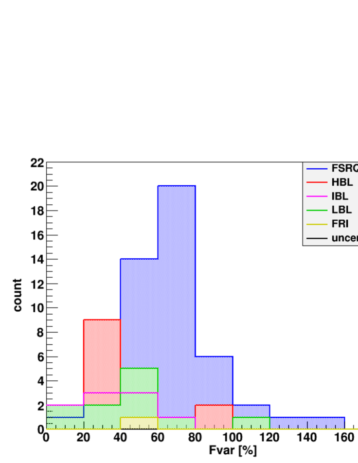
Figure 3: The $F_{\rm var}$ distribution. The width of $F_{\rm var}$ bin is 20%. The different colors show each subclass of blazars (Blue: FSRQ, Red: HBL, Magenta: IBL, Green: LBL, Yellow: FRI, Black: uncertain type.).

V CONCLUSIONS

We selected 102 AGNs (blazars) to reveal the relation between the evolution process of AGNs and the blazar sequence. We applied the fractional variability amplitude ($F_{\rm var}$) to calculate the variability amplitude considering the error.
The analyzed AGNs were selected from the second LAT AGN catalog (2LAC)2LAC and TeVCatTeVCat . The analyzed data was Fermi reprocessed pass 7 data between 2008 August 04 and 2014 June 09, using the unbinned likelihood analysis with the Fermi Science Tools.
From these features, blazar subclass seems to change along the increasing redshift (connection with FSRQs $\rightarrow$ LBLs $\rightarrow$ HBLs (IBLs)). This trend shows possibility of the activity evolution and blazar class evolution. Peculiar features were as follows; AO 0235+164 (z = 0.94, LBL) has particularly high $F_{\rm var}$ (117 $\pm$ 2.8) in LBLs. This source was discussed that it might be FSRQ type blazar Ackermann2012 ; Stickel1994 ; therefore, high $F_{\rm var}$ value of this source might be caused by the FSRQ like characters. S3 0218+357 (z = 0.944, Uncertain type) which has the highest $F_{\rm var}$ (190 $\pm$ 2.8) in this analyzed sources is a gravitationally lensed blazarS3Atel , hence the very high $F_{\rm var}$ value might be enhanced by the gravitationally lensed effect.
However, there are some problems in this study. First, the middle-high redshift (z $>$ 0.2) low $F_{\rm var}$ sources were not sufficient for discussions without selection effects. Second, this study could not considered the short time scale variability ($<$ 30days). Thus, It is necessary to analyze the low $F_{\rm var}$ sources and short time scale.

References

- (1) M. Ackermann et al., ApJ, 751, (2012) 159
- (2) M. Elvis, et al., ApJS, 80, (1992) 257
- (3) Fermi-LAT Collaboration, ApJ, 743,(2011) 171
- (4) G. Fossati, et al., MNRAS, 299, (1998) 433
- (5) A. Furniss, ApJ, 768, (2013) 6
- (6) H. Kür, et. al, A&A, 45, (1981) 367
- (7) MAGIC Collaboration, arXiv:1409.3389 (2014)
- (8) P. Padovani and C.M. Urry, ApJ, 387, (1992) 449
- (9) J. Poutanen, et. al, MNRAS, 1427, (2008) 389
- (10) M. Stickel, et al., A&A Suppl. Ser., 105, (2014) 211
- (11) S. Vaughan, et. al, MNRAS, 345, (2003) 1271
- (12) http://tevcat.uchicago.edu/
- (13) http://fermi.gsfc.nasa.gov/ssc/
-
(14)
http://fermi.gsfc.nasa.gov/ssc/data/access/lat/
BackgroundModels.html -
(15)
http://fermi.gsfc.nasa.gov/ssc/data/analysis/
documentation/Cicerone/Cicerone_Data_Exploration
/Data_preparation.html -
(16)
http://fermi.gsfc.nasa.gov/ssc/data/analysis/
scitools/source_models.html - (17) http://www.astronomerstelegram.org/?read=6349