Molecular Density Functional Theory for water with liquid-gas coexistence and correct pressure

Abstract

The solvation of hydrophobic solutes in water is special because liquid and gas are almost at coexistence. In the common hypernetted chain approximation to integral equations, or equivalently in the homogenous reference fluid of molecular density functional theory, coexistence is not taken into account. Hydration structures and energies of nanometer-scale hydrophobic solutes are thus incorrect. In this article, we propose a bridge functional that corrects this thermodynamic inconsistency by introducing a metastable gas phase for the homogeneous solvent. We show how this can be done by a third order expansion of the functional around the bulk liquid density that imposes the right pressure and the correct second order derivatives. Although this theory is not limited to water, we apply it to study hydrophobic solvation in water at room temperature and pressure and compare the results to all-atom simulations. The solvation free energy of small molecular solutes like $n$-alkanes and hard sphere solutes whose radii range from angstroms to nanometers is now in quantitative agreement with reference all atom simulations. The macroscopic liquid-gas surface tension predicted by the theory is comparable to experiments. This theory gives an alternative to the empirical hard sphere bridge correction used so far by several authors.

I Introduction

Implicit solvation techniques based on liquid-state theory such as integral equation theory in the interaction-sitechandler_optimized_1972 ; hirata_application_1982 or molecular pictureblum_invariant_1972 ; blum_invariant_1972-1 or classical density functional theoryevans_nature_1979 ; evans_density_2009 ; henderson_fundamentals_1992 have proven to be successful for the computation of solvation properties. Those methods have shown to give thermodynamic and structural results that get closer and closer to all-atom simulations at a much lower numerical cost. A current challenge lies in the development and implementations of three-dimensional implicit solvation theories to describe molecular liquids and solutions. Recent developments in this direction have focused on Gaussian fieldvarilly_improved_2011 theoretical approaches, or the 3D reference interaction site model (3D-RISM),beglov_integral_1997 ; hirata_molecular_2003 an appealing integral equation theory that has proven recently to be applicable to, e.g., structure prediction in complex biomolecular systems. Integral equations are, however, restricted by the choice of a closure relation, typically, Hypernetted Chain (HNC), Percus-Yevick or Kovalenko-Hirata. Despite their great potential, they remain difficult to control and improve, especially for arbitrary three-dimensional molecules, and they can prove difficult to converge.

We have proposed recently a three dimensional formulation of molecular density functional theory (MDFT) in the homogeneous reference fluid approximation (HRF) to study solvationramirez_density_2002 ; jeanmairet_molecular_2013-1 . It has proven successful in studying solvation properties of solutes of arbitrary three-dimensional complexity embedded in various molecular solvents. However, when one comes to water, the HRF approximation fails even qualitatively to predict the solvation of large hydrophobic solutesjeanmairet_molecular_2013 . Such limitation can be explained by two essential features of water at ambient conditions that are not properly described by HRF functional. First, it is known that the solvation free energy of mesoscale apolar solutes can be modeled as the sum of a surface and volume termreiss_statistical_1959 . For water, as well as for any solvent at room condition, the pressure is very low, inducing negligible $PV$ term until large radiihuang_scaling_2001 . Another key feature is that at ambient condition, water is close to its liquid-gas coexistence. As a consequence the solvation of big hydrophobic solutes may induce dewetting huang_hydrophobic_2002 .

In section II, we propose an extension of MDFT to introduce the liquid-gas coexistence of the solvent and to recover the correct pressure. Then, in section III, we apply our theory to a model of water and compare the results of solvation of apolar solutes with reference all-atom Monte Carlo simulations (MC).

II Theory

While the theory discussed here is generic to any classical density functional theory, it is described below in the framework of the MDFT for water introduced recentlyjeanmairet_molecular_2013-1 ; jeanmairet_molecular_2013 . We start from the single point charge extended (SPC/E) model of waterberendsen_missing_1987 , that is, a model comprising one Lennard-Jones site and 3 partial charges. With MDFT, one computes the solvation free energy and the solvation structure of a solute of arbitrary shape that acts on the water density field through an external potential. This last quantity is the sum of an electrostatic vector field $\boldsymbol{E}(\boldsymbol{r})$ and a Lennard-Jones scalar field $\Phi_{\mathrm{LJ}}(\boldsymbol{r})$jeanmairet_molecular_2013-1 . In the general case, the functional of the density $\rho(\boldsymbol{r},\boldsymbol{\Omega})$ depends upon the position $\boldsymbol{r}$, and the molecular orientation of the (rigid) solvent molecule. There is no restriction on the molecular or chemical nature of the solvent molecule model, but to be rigid. In that particular model of water, $\rho(\boldsymbol{r},\boldsymbol{\Omega})$ can be split into two distinct fields: the molecular density field $n(\boldsymbol{{r}})$ coupled to $\Phi_{\mathrm{LJ}}(\boldsymbol{r})$ and the polarization vector field $\boldsymbol{P}(\boldsymbol{r})$ coupled to $\boldsymbol{E}\left(\boldsymbol{r}\right)$. These fields are themselves functionals of $\rho(\boldsymbol{r},\boldsymbol{\Omega})$:

$$n(\boldsymbol{{r}})=\int\rho(\boldsymbol{r},\boldsymbol{\Omega})\mathrm{d\boldsymbol{\Omega}},$$ (1)

$$\boldsymbol{P}(\boldsymbol{r})=\iint\rho(\boldsymbol{r}^{\prime},\boldsymbol{\Omega})\boldsymbol{\mu}(\bm{r}-\bm{r}^{\prime})\mathrm{d\boldsymbol{r}}^{\prime}\mathrm{d\boldsymbol{\Omega}}.$$ (2)

where $\mathrm{d\boldsymbol{\Omega}}$ denotes the integration over all molecular orientations. $\boldsymbol{\mu}(\boldsymbol{r},\boldsymbol{\Omega})\equiv\sum_{\text{m}}q_{\text{m}}\bm{s}_{\text{m}}(\bm{\Omega})\intop_{0}^{1}\delta(\bm{r}-u\bm{s}_{\text{m}}(\bm{\Omega}))\text{d}u$ is the molecular polarization of a single water molecule at the origin of a cartesian frame, $q_{\mathrm{m}}$ and $\bm{s}_{\text{m}}$ are the charge and position of the m^th solvent site. One should refers to Jeanmairet et aljeanmairet_molecular_2013-1 for a complete description of MDFT for water. Without loss of generality, we will stick in what follows to solutes without partial charges, so that the polarization vector field is zero $\left(\boldsymbol{P}=\boldsymbol{0}\right)$. As a consequence, the free energy is, at dominant order, a functional of $n(\boldsymbol{{r}})$ only.

We now write the Helmholtz free energy functional, ${\cal F}[n]$, that is the difference of the grand potential of the system containing the solute, $\Theta$, and without the solute, $\Theta_{\mathrm{B}}$. In this last case, the solvent is homogeneous at density $n_{\textrm{B}}$ (typically 1 g/cm³ for water):

$${\cal F}[n]=\Theta[n]-\Theta_{\mathrm{B}}.$$ (3)

This leads to

$${\cal F}[n(\boldsymbol{{r}})] =\mathrm{k_{B}}T\int\left[n(\boldsymbol{{r}})\ln\left(\frac{n(\boldsymbol{{r}})}{n_{\mathrm{B}}}\right)-n(\boldsymbol{{r}})+n_{\mathrm{B}}\right]\mathrm{d\boldsymbol{r}}$$

$$+\int n(\boldsymbol{{r}})\Phi_{\mathrm{LJ}}(\boldsymbol{r})\mathrm{d\boldsymbol{r}}+{\cal F_{\mathrm{exc}}^{\ }}[n(\boldsymbol{{r}})].$$ (4)

The terms of the right-hand side of Eq.4 corresponds to the usual decompositionevans_nature_1979 ; evans_density_2009 ; henderson_fundamentals_1992 into an ideal term accounting for information entropy, an external term accounting for the perturbation by the solute through its external potential, and an excess term accounting for solvent-solvent correlations. This last, excess term, can be rewritten without additional approximation as

$${\cal F_{\mathrm{exc}}^{\ }}[n(\boldsymbol{{r}})] =-\frac{\mathrm{k_{B}}T}{2}\iint\Delta n(\boldsymbol{{r}})c(r)\Delta n(\boldsymbol{r}^{\prime})\mathrm{d\boldsymbol{r}}\mathrm{d\boldsymbol{r}}^{\prime}+{\cal F_{\mathrm{b}}^{\ }}$$ (5)

$$={\cal F_{\mathrm{exc}}^{\mathrm{HNC}}}+{\cal F_{\mathrm{b}}^{\ }},$$

where $r\equiv\left\|\boldsymbol{r}-\boldsymbol{r}^{\prime}\right\|$, $\Delta n(\boldsymbol{{r}})\equiv n(\boldsymbol{{r}})-n_{\mathrm{B}}$, and $c(r)$ is the direct correlation function of the homogeneous reference fluid at density $n_{\mathrm{B}}$. The first term thus corresponds to a series expansion in density of ${\cal F_{\mathrm{exc}}^{\ }}$, around the density of the HRF, truncated at second order. Truncated information is put into an unknown bridge term, ${\cal F_{\mathrm{b}}^{\ }}$. When ${\cal F_{\mathrm{b}}^{\ }}=0$ , i.e. when we stick to the pure HRF approximation, Eq.5 can be shown to correspond to the HNC approximation of integral equationshansen_theory_2006 . It will thus be called the HNC functional below. We suppose now that the correction can be expressed as a polynomial containing all terms of orders higher than 2 in $\Delta n$. Eq.5 can be used only if one knows the direct correlation function, $c(r)$. In this article, we use an accurate direct correlation function of SPC/E water computed by Belloni et al. according to the methods discussed in refs.  puibasset_bridge_2012 ; belloni_efficient_2014 . The Fourier transform of the direct correlation function, $\hat{c}$, is calculated by

$$\hat{c}\left(k\right)=\frac{\hat{h}_{000}\left(k\right)}{1+n_{B}\hat{h}_{000}\left(k\right)},$$ (6)

where $\hat{h}_{000}\left(k\right)$ is the first rotational invariant of the Fourier transform of the total correlation function $h$ calculated by Puibassset and Belloni puibasset_bridge_2012 . This function, as well as all higher rotational invariant components are obtained at short range by Monte Carlo sampling, and at higher range by integral equation closures, so that small $k$ values are very accurate.

The HNC functional has proved to be good enough for studying solvation in acetonitrile and in the Stockmayer fluid, but it exhibits wrong behaviors when coming to waterzhao_molecular_2011 . To improve the description of water we have proposed, as several other authors _fast_Wu_2014 ; oettel_integral_2005 , an hard sphere bridge functional that consists in replacing all the unknown orders in $\Delta n$ of the molecular fluid by the known ones of a hard sphere fluid of a diameter chosen on physical considerationslevesque_scalar_2012 . Such a correction does improve the solvation of small molecular solutes zhao_new_2011 ; zhao_correction_2011 ; levesque_scalar_2012 . However, the HNC functional or the functional with the hard sphere bridge, HNC+HSB, are not able to reproduce to date the solvation of hydrophobic solutes at both small and large length scales. This is an important discrepancy that originates from the fact that water at room conditions is close to liquid-gas coexistence and has a very low pressure, a fact that is impossible to account for consistently in HNC oettel_integral_2005 .

We proposed recently a correction that imposes the essential physicsjeanmairet_molecular_2013 . It is based on the separation of the functional of Eq.4 with the hard sphere correction in a short range and a long range part. The long range part was then made compatible with the Van-der-Waals theory of phase coexistence at long range in a spirit similar to the Lum-Chandler-Weeks theorylum_hydrophobicity_1999 . It introduces a coarse-grained density, similar in nature to weighted densities at the core of fundamental measure theories for hard sphere fluidsrosenfeld_free-energy_1989 . We were then able to reproduce qualitatively the solvation of hydrophobic solutes at all length-scales. The surface tension was found too high, however, and the solvation structure of qualitative agreement only. It should be noted that the key role of the pressure of the fluid was not identified in this work: The pressure was consequently not explicitly considered as a control parameter even if this correction had an effect on the pressure. A functional that imposes the coexistence and the right pressure of the fluid is thus presented here.

What we propose is an expression of ${\cal F_{\mathrm{b}}^{\ }}$ that is cubic in $\Delta n$. There are two main motivations to such an expression. (i) First, Evans et alevans_failure_1983 and later Rickayzen and collaboratorsrickayzen_integral_1984 ; powles_density_1988 showed that a series expansion of the functional at the quadratic order is thermodynamically inconsistent . In particular, the pressure of the homogeneous reference fluid predicted by the theory can be overestimated by orders of magnitude. For instance, for water, the HNC functional predicts a pressure of approximately 11450 bar instead of 1 bar. (ii) Also, Rickaysen proposed to add the simplest cubic term to the series expansion of $\mathcal{F}_{\mathrm{exc}}$ in density, and showed it to be sufficient to overcome the thermodynamic inconsistency. Following Rickayzen’s prescriptions, a “three body” bridge term that is cubic in $\Delta n$, $\mathcal{F}_{3\mathrm{B}}$, is proposed. We give arguments on the form that should have $\mathcal{F}_{3\mathrm{B}}$ for water, and how the addition of a physical constraint makes it a single parameter functional.

Instead of the simple three body expression of Rickayzen based on the overlap of hard bodies, we use here a rather different expression that is motivated by the fact that in water, tetrahedral order due to hydrogen bonding is lost in the HNC approximation and should be reinforced. Note that if the structuration discussed below is particular to water, the idea of including a three body term to improve the local structuration given by the HNC functional is relevant for any solvent.

The three body functional should (i) enforce thermodynamic consistency, (ii) give back the local order due to $N$-body interactions missed so far ($N>2$), and (iii) stay numerically efficient since it is our long-term goal to compete with other implicit methods like PCM (Polarizable Continuum Model)tomasi_quantum_2005 that are much cruder but extremely useful. This last point may seem minor from a physical point of view; Nevertheless, to compute $\mathcal{F}_{3\mathrm{B}}$, one should integrate over the whole $\mathbb{R}^{9}$ instead of $\mathbb{R}^{6}$ (with convolutions) for HNC: if it is not built efficiently, then it is useless. Consequently, in addition to physical motivation, the analytical form of the three body functional introduced here must allow efficient computation.

We start from the idea of the coarse-grained model of tetracoordinated silicon by Stillinger and Weberstillinger_computer_1985 ; stillinger_erratum:_1986 , re-parameterized later for water by Molinero and Mooremolinero_water_2009 . Their idea relies on an harmonic penalty to non-tetrahedral oxygen-oxygen-oxygen angles. In the MDFT framework, it leads to

$$\beta{\cal F_{\mathrm{3B}}^{\ }}[n(\bm{r})] =\frac{\lambda}{2}\int\Delta n(\bm{r}_{1})\biggl{[}\iint\Delta n(\bm{r}_{2})\Delta n(\bm{r}_{3})f(r_{12})f(r_{13})$$

$$\times\left(\frac{\bm{r}_{12}\cdot\bm{r}_{13}}{r_{12}r_{13}}-\cos\theta_{0}\right)^{2}\mathrm{d}\bm{r}_{2}\mathrm{d}\bm{r}_{3}\biggr{]}\mathrm{d}\bm{r}_{1},$$ (7)

with $\beta$=($\mathrm{k_{B}}T$)^-1. The dot product defines the cosine of the angle between three space points, and the quadratic term enforces a tetrahedral angle with $\theta_{0}=109.5\text{\textdegree}$. The function $f$ tunes the range of the three body interaction. As a source of local structuration of the fluid, it must be short-ranged and must vanish after few solvent radii, at distance $r_{\mathrm{max}}$. We propose as Molinero and Moore

$$f(r)=\begin{cases}\exp\left(\frac{2}{3}\frac{r_{\mathrm{max}}}{\left(r-r_{\mathrm{max}}\right)}\right)&\text{if $r<r_{\mathrm{max}}$}\\ 0&\text{if $r\geq r_{\mathrm{max}}$}\end{cases}.$$ (8)

$\lambda$ is a dimensionless parameter modulating the strength of this oriented-bond term (hydrogen bond in case of water). The excess term in Eq.7 is specific to a given fluid and should thus be parameterized once for all for the sake of consistency. We chose it so that one recovers the thermodynamic consistency and the correct pressure of the bulk liquid.

The grand potential of a system of homogeneous fluid of volume $V$ and pressure $\mathrm{P}$ is equal, by definition, to $-\mathrm{P}V$. It is $0$ in an empty system. Thus, one can deduce the pressure in the reference fluid by evaluating the functional of Eq.4 at zero densitysergiievskyi_fast_2014 :

$${\cal F}[n=0]=\Theta[n=0]-\Theta_{\mathrm{B}}=\mathrm{P}V,$$ (9)

Using Eq.9 for the functional without the three body term we get,

$$\beta\mathrm{P_{HNC}}=n_{\mathrm{B}}-\frac{n_{\mathrm{B}}^{2}}{2}\bar{c}$$ (10)

with $\bar{c}=4\pi\int_{0}^{\infty}r^{2}c(r)\mathrm{d}r$. With the three-body term:

$$\beta\mathrm{P_{3B}}=n_{\mathrm{B}}-\frac{n_{\mathrm{B}}^{2}}{2}\bar{c}+\frac{32n_{\mathrm{B}}^{3}}{9}\pi^{2}\lambda\left[\int_{0}^{\infty}f(r)r^{2}\mathrm{d}r\right]^{2}.$$ (11)

With Eq.10 we find a pressure above 11450 bar for the HNC functional. Eq.11 is used to fix the parameter $\lambda$ to have the desired pressure for the bulk fluid, i.e., 1 bar for water at room conditions. With this constraint, the three body functional has only one parameter left: the range of the interaction, $r_{\mathrm{max}}$. Molinero and Moore determined a parameter $r_{\mathrm{max}}=4.3$ Å  for their model. We kept the freedom of slightly varying $r_{\mathrm{max}}$ around this value. An optimum value is found for $4.2$ Å. See below.

The direct computation of the three-body function of Eq.7 cannot be performed because it requires a triple nested integration over the spacial coordinates. To accelerate the computation of this term we rewrite Eq.7 as:

$$\beta{\cal F_{\mathrm{3B}}^{\ }}[n(\bm{r})] =\frac{\lambda}{2}\int\Delta n(\bm{r}_{1})\left(\sum_{\alpha,\beta\in\left\{x,y,z\right\}}\bar{n}_{\alpha\beta}(\bm{r}_{1})^{2}+\cos^{2}\left(\theta_{0}\right)\bar{n}{}_{0}(\bm{r}_{1})^{2}-2\cos\left(\theta_{0}\right)\bar{\bm{n}}_{1}(\bm{r}_{1})\cdot\bar{\bm{n}}_{1}(\bm{r}_{1})\right)\mathrm{d}\bm{r}_{1}$$ (12)

where

$$\bar{n}_{\alpha\beta}(\bm{r}_{1})=\int f(r_{12})\frac{\alpha_{12}\beta_{12}}{r_{12}^{2}}\Delta n(\bm{r}_{2})\mathrm{d}\bm{r}_{2}\text{, \ $\alpha,\beta\in\left\{x,y,z\right\}$}$$ (13)

$$\bar{\bm{n}}_{1}(\bm{r}_{1})=\int f(r_{12})\frac{\bm{r}_{12}}{r_{12}}\Delta n(\bm{r}_{2})\mathrm{d}\bm{r}_{2},$$ (14)

$$\bar{n}{}_{0}(\bm{r}_{1})=\int f(r_{12})\Delta n(\bm{r}_{2})\mathrm{d}\bm{r}_{2}.$$ (15)

It can be seen that ${\cal F_{\mathrm{3B}}^{\ }}$ belongs to the general class of weighted functionals with one scalar weighted density, one vectorial one, and one second order, tensorial one.

The derivation of the equivalence between Eq.7 and Eq.12 as well as the first- and second-order functional derivatives that may be needed for minimizing Eq.7 are given in supplementary informationSeeSup . Convolution products of Eqs.13, 14 and 15 are evaluated efficiently in three dimensions using fast Fourier transforms (FFT). We typically use cubic boxes of $35^{3}$ ų with space discretized by 5 grid nodes per Å. Functional minimization of the total functional is typically reached within 15 to 20 iterations in a few tens of minutes on a single processor core at 2.4 GHz.

III Results and Discussion

Our goal is to predict the hydration structure and free energy of hydrophobic solutes from microscopic to macroscopic length scales. Hydration free energies of nanometric solutes are proportional to the surface of the solute. Since this behavior is due to the almost zero pressure of liquid water at room conditions, it is of prime importance to build a density functional that imposes the right pressure. First, we describe the parameterization of Eq.7 for capturing both the liquid-gas coexistence and the correct pressure. After that, we test the functional against hydration of various apolar solutes.

To parametrize and test the three body term of Eq.7 we first study small molecular apolar solutes. In Fig.1, we show the solvation free energies of small alkane chains as computed by Monte Carlo simulations (MC)ashbaugh_hydration_1998 and by MDFT-HNC or MDFT-HNC+3B with $r_{\mathrm{max}}=4.3$ Å and $4.2$ Å. Within MDFT-HNC, the error in solvation free energy increases linearly with the size of the alkane, that is its number of carbons, shown here from methane to hexane. With the three-body excess functional, the relative error of MDFT with respect to Monte Carlo simulations is reduced by several orders.

We find that $r_{\mathrm{max}}=4.2$ Å produces the optimal results, close to $4.3$ Å  for Molinero and Moore and we stick to this value in the rest of the article. The remaining parameter $\lambda$ is chosen to impose the correct pressure in bulk water, $\mathrm{P}=1$ bar, from Eq.11. One finds $\lambda=38$. We highlight that since the pressure of the fluid is now correct, the pressure correction term proposed by Sergiievskyi et alsergiievskyi_fast_2014 is no longer required.

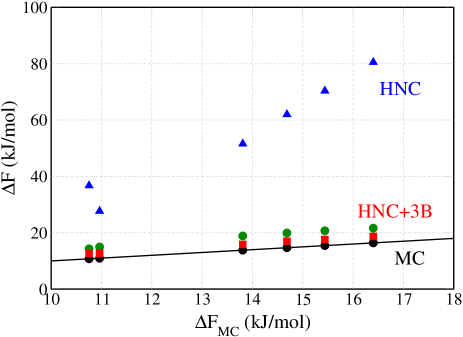
Figure 1: Hydration free energies for the first six linear alkanes as calculated with MDFT-HNC and MDFT-HNC+3B, compared to Monte Carlo simulations by Ashbaugh et. al. ashbaugh_hydration_1998 . $r_{\mathrm{max}}=4.2$ Å (red squares) and $4.3$ Å  (green circles) are shown for MDFT-HNC+3B.

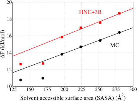
Figure 2: Hydration free energy in SPC/E water for the first six linear alkanes as a function of the solvent accessible surface area (SASA). Reference results from Monte Carlo are plotted as black circles. MDFT results with three-body corrections are in red squares. Linear regressions based on propane, butane, pentane and hexane are also plotted.

The solvation free energy of $n$-alkanes into water is known to scale linearly with the molecular surface area bennaim_solvation_1984 ; ashbaugh_hydration_1998 :

$$\Delta\mathrm{F}=\gamma_{\textrm{m}}\mathcal{A}+b,$$ (16)

with $\mathcal{A}$ the solute area, $\gamma_{\textrm{m}}$ the free energy per microscopic surface area and $b$ an offset. Note that $\gamma_{\textrm{m}}$ is a microscopic equivalent to a surface tension, but is definitely different from the macroscopic liquid-gas surface tension. Several definitions of $\mathcal{A}$ can be found in the litterature, that do not change any conclusion therein: We will use the solvent accessible surface area (SASA) of water in what follows, in order to be as comparable as possible with the results by Ashbaugh et al. ashbaugh_hydration_1998 . The evolution of the hydration free energy with respect to the solvent accessible surface area is plotted in Fig.2. With the three-body excess functionnal, we now find the anticipated linear dependancy. The values $\gamma_{\textrm{m}}$ and $b$ given by the linear regressions corresponding to equation 16 are given in Table 1. The value of $\gamma_{m}$ is in good agreement with both MC and experiments. We get an offset of approximately one $\mathrm{k_{B}}T$ with respect to MC.

	HNC	HNC+3B	MD	Exp.
$\gamma_{m}$ (J/(mol$\cdot$Å2))	$340.59$	$32.49$	$30.53$	$28.5$
$b$ (kJ/mol)	$-15.02$	$9.52$	$7.81$	$2.51$

Table 1: Microscopic equivalent to the surface tension and offset from MD ashbaugh_hydration_1998 , from experimentsbennaim_solvation_1984 and by MDFT-HNC and MDFT-HNC+3B.

Now that parameters are fixed once for all, we show in Fig.3 the Helmholtz free energy of the homogenous systems as a function of the density at 300 K, as computed with the MDFT-HNC functional in dashed red and with the MDFT-HNC+3B functional in black. As discussed above, no second phase can appear in the system described with the MDFT-HNC functional since the free energy has only one minimum. Consequently, it can not capture liquid-gas coexistenceevans_failure_1983 . On the other hand, there are two minima of the Helmholtz free energy for the functional that includes the three-body bridge functional. A local minimum is found close to zero-density (“a gas phase”) with a free energy larger than the one of the global minimum corresponding to the density of the reference homogeneous fluid. The difference in Helmholtz free energy is of the order of $6.0.10^{-5}$ kJ/ų, the homogeneous water we are describing is thus liquid and very close to liquid-gas coexistence. This physical feature is a key dzubiella_competition_2004 to predict the solvation structure of large hydrophobic solutes of nanometer scale.

To summarize: (i) the cost in free energy per unit volume for creating a cavity within the HNC (or HRF) formalism is several orders of magnitude too high, in relation to its overestimation of the pressure, (ii) the bridge functional that we propose corrects both the local order and the pressure, and it induces that the system is close to coexistence. The cost for creating a cavity within the MDFT-HNC+3B formalism is thus reduced to almost zero.

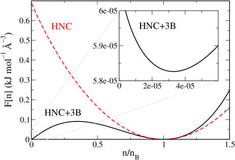
Figure 3: Helmholtz free-energy of a homogeneous system of density $n$, see Eq. 4. $n_{\mathrm{B}}$ is the reference density one uses for the HNC functional. The insight is a focus on the first local minimum of the three-body corrected functional, HNC+3B.

We now focus on the solvation of hydrophobic solutes of atomic to nanoscale sizes. In their seminal works, Chandler and collaboratorslum_hydrophobicity_1999 ; huang_hydrophobic_2002 studied by Monte Carlo simulations the hydration of hard spheres whose radii range from angstroms to nanometers. They observed a maximum in height of the first peak of the hard sphere - water radial distribution function at approximately 5 Å. For radii larger than about 10 Å, they also observed a slow convergence toward a plateau for the surface free energy. We compare the results by MDFT-HNC and MDFT-HNC+3B to those of Huang et al. in Fig.4, Fig.5 and Fig.6. One should keep in mind that MDFT results are approximatively 1000 times faster than explicit molecular dynamics or Monte Carlo simulations and that no other implicit solvent methods besides the LCW theory is able to reproduce these thermodynamic properties.

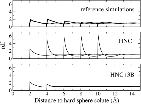
Figure 4: Radial distribution function of a hard sphere solute of growing radius in SPCE water at 300 K from reference Monte Carlo simulations huang_hydrophobic_2002 , MDFT-HNC and MDFT-HNC+3B.

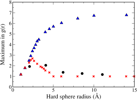
Figure 5: Maxima of the radial distribution functions of hard sphere of different radii $R$. The MC simulations results of Huang et al. huang_hydrophobic_2002 are the black circles, the ones obtained by MDFT-HNC+3B are the red crosses and the results of MDFT-HNC are the blue triangles.

In Fig.5, we present the evolution of the height of the first peak of the hard sphere (HS) - water radial distribution function when the HS radius increases. This maximum corresponds to the most probable distance of molecules of the first solvation shell to the center of the hard sphere solute. The reference data by explicit methods are given in black huang_hydrophobic_2002 . This height exhibits a peculiar maximum that is characteristic of the solvation of hydrophobic solutes in waterdzubiella_competition_2004 . It tends toward unity for large radii. This behavior has been explained as follow: for small radii, the solvent can reorganize around the solute without losing solvent-solvent interactions, that is without losing too much cohesion: The increase of the height of the peak is due to an increase in packing of molecules at the surface of the sphere. For bigger radii, the perturbation is too high to keep the local structure unchanged: there is a loss of solvent-solvent interactions that has an energetic cost that limits the accumulation of molecules at the surface of the sphere and induces dewetting eventually. As a summary, when the perturbation stays small compared to solvent cohesion, the packing increases around the solute. Then, when the perturbation (the size of the solute) is unfavorable compared to solvent cohesion, solvent molecules stand back and the packing decreases.

MDFT-HNC fails to reproduce this behavior: as depicted in Fig.3 there is no possible change of regime for the fluid. With the three body term, this change of regime can be found if the perturbation is able to make the fluid reach a state close to the second minimum. This is confirmed by Fig.5, where MDFT-HNC+3B is in qualitative agreement with reference all atom simulations: The maximum of the radial distribution function is obtained around $2.5\ \textrm{\AA}$, which is reasonable a value. The decrease is, however, too fast.

In Fig.6 we plot the solvation free energy of HS solutes per surface unit. We compile therein the results by MDFT-HNC, MDFT-HNC+3B and once again the reference all atom Monte Carlo simulations. MC shows a linear increase of the surface free energy for small radii, followed by a transition state, then followed by a plateau. This asymptotic value, reached at large HS radii corresponds to the surface tension of the fluid. At this regime, the solvation is thus driven by a sole surface term that corresponds at the microscopic level to the case where the loss of interaction between solvent particles is the prominent energetic term. MDFT-HNC is in agreement with the simulations only for very small radius (below $2.5\ \textrm{\AA}$) but does not reproduce the plateau for bigger radius ($>10\ \textrm{\AA}$), this is consistent with the structural results, the transition between the two regimes is missed. Again, MDFT-HNC+3B is in good agreement with the simulations and the surface tension of SPC/E water estimated by Vega et al vega_surface_2007 is recovered.

We can thus relate the decay of the maximum of the radial distribution function in Fig.5 and the convergence to the plateau in Fig.6. For structural and energetic properties, Monte Carlo simulations show a smooth transition between the two regimes described above, while MDFT-HNC+3B sharpens the transition: The three body term exacerbates the importance of the loss of attraction between solvent molecules.

To conclude this section, (i) the structural properties obtained with MDFT-HNC+3B are improved with respect to MDFT-HNC since we recover the change in regime observed in MC at least qualitatively; (ii) this is also true for the the solvation free energy and this represents a considerable progress since MDFT-HNC predicts the wrong quantitative behavior. (iii) The surface tension, that is related to the height of the saddle point in the free energy curve of Fig.3, is correctly reproduced by MDFT-HNC+3B even though this is not explicitly controlled.

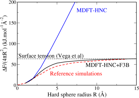
Figure 6: Solvation free energy for hard spheres of different radii $\mathrm{R}$. The value of the liquid-vapor surface tension of SPC/E water at 300 K estimated by Vega et alvega_surface_2007 (63.6 mJ/m²) is shown in dotted black line. MDFT-HNC+3B gets the right behavior: two regimes at small then large HS radii, and the correct surface tension.

IV Conclusions

In this paper, we propose to go beyond the usual quadratic expansion of the Gibbs free energy (or equivalently of the excess functional) around the homogeneous reference fluid within the molecular density functional theory framework. We thus go beyond the HNC approximation. MDFT-HNC+3B imposes a second local minimum to the Gibbs free energy of the system at low fluid density. The bridge functional that was proposed (i) enforces the tetrahedral order of water, (ii) recovers the close coexistence between gas and liquid states and their surface tension, and (iii) is consistent with the experimental pressure of the fluid. It introduces one empirical parameter that we fix to parameterize over the solvation free energy of the first linear alkanes. It recovers the reference results of explicit simulations with a systematic offset of order $\mathrm{k_{B}}T$. That is close to chemical accuracy, and is a clear improvement over MDFT-HNC.

One advantage of this additional term with respect to previous workjeanmairet_molecular_2013 is that (i) it has a single empirical parameter, (ii) it does not require additional fields like coarse-grained densities, and (iii) it makes the theory thermodynamically consistent.

This bridge functional was used to study the solvation free energy of hard spheres whose radii range from angstroms to nanometers. Unlike MDFT-HNC, MDFT-HNC+3B recovers the change of regime between a solvation governed by distortion of the solvent structure and a solvation governed by a complete reorganization of the solvent. The free energy of solvation and the surface tension are correct. Nevertheless, the transition stage is too sharp.

Indeed, this points out the necessity of further improvements of the functional. Other thermodynamic properties pertinent to hydrophobic solvation, such as entropy, enthalpy, partial molar volumes, temperature dependence, remain to be carefully tested too.

Numerical efficiency is the very essence of implicit methods like MDFT. The bridge functional introduced therein would cause a dramatic increase of the numerical cost without its rewriting in terms of fast Fourier transforms. This is an important result of this article. The numerical cost increase is at this stage of one order of magnitude only with respect to MDFT-HNC. MDFT-HNC+3B is still two to three orders of magnitudes faster than explicit simulations.

Finally the solutes studied here are all apolar and neutral, for the sake of clarity and pedagogy. The three-body functional is built to account for short-range tetrahedral order in the solvent. It is similar in spirit to solute-solvent corrections that were introduced previously in the group to describe ions and H-bonded polar solutes jeanmairet_molecular_2014 ; jeanmairet_molecular_2013-1 ; jeanmairet_molecular_2013 . We think this will lead to a consistent functional for water, valid for both hydrophobic and hydrophilic interactions.

- [1] David Chandler and Hans C. Andersen. Optimized cluster expansions for classical fluids. II. theory of molecular liquids. The Journal of Chemical Physics, 57(5):1930–1937, 1972.
- [2] Fumio Hirata, B. Montgomery Pettitt, and Peter J. Rossky. Application of an extended RISM equation to dipolar and quadrupolar fluids. J. Chem. Phys., 77(1):509–520, 1982.
- [3] L. Blum. Invariant expansion. II. the ornstein-zernike equation for nonspherical molecules and an extended solution to the mean spherical model. The Journal of Chemical Physics, 57(5):1862–1869, 1972.
- [4] L. Blum and A. J. Torruella. Invariant expansion for two-body correlations: Thermodynamic functions, scattering, and the ornstein—zernike equation. The Journal of Chemical Physics, 56(1):303–310, 1972.
- [5] R. Evans. The nature of the liquid-vapour interface and other topics in the statistical mechanics of non-uniform, classical fluids. Advances in Physics, 28(2):143, 1979.
- [6] R. Evans. Density functional theory for inhomogeneous fluids i: Simple fluids in equlibrium. In Lecture notes at 3rd Warsaw School of Statistical Physics. 2009.
- [7] R. Evans. Fundamentals of Inhomogeneous Fluids. Marcel Dekker, Incorporated, 1992.
- [8] Patrick Varilly, Amish J. Patel, and David Chandler. An improved coarse-grained model of solvation and the hydrophobic effect. The Journal of Chemical Physics, 134(7):074109–074109–15, 2011.
- [9] Dmitrii Beglov and Benoît Roux. An integral equation to describe the solvation of polar molecules in liquid water. J. Phys. Chem. B, 101(39):7821–7826, 1997.
- [10] F. Hirata. Molecular Theory of Solvation. Springer, 2003.
- [11] Rosa Ramirez, Ralph Gebauer, Michel Mareschal, and Daniel Borgis. Density functional theory of solvation in a polar solvent: Extracting the functional from homogeneous solvent simulations. Phys. Rev. E, 66(3):031206–031206–8, 2002.
- [12] Guillaume Jeanmairet, Maximilien Levesque, Rodolphe Vuilleumier, and Daniel Borgis. Molecular density functional theory of water. J. Phys. Chem. Lett., 4:619–624, 2013.
- [13] Guillaume Jeanmairet, Maximilien Levesque, and Daniel Borgis. Molecular density functional theory of water describing hydrophobicity at short and long length scales. The Journal of Chemical Physics, 139(15):154101–1–154101–9, 2013.
- [14] H. Reiss, H. L. Frisch, and J. L. Lebowitz. Statistical mechanics of rigid spheres. The Journal of Chemical Physics, 31(2):369–380, 1959.
- [15] David M. Huang, Phillip L. Geissler, and David Chandler. Scaling of hydrophobic solvation free energies. J. Phys. Chem. B, 105(28):6704–6709, 2001.
- [16] David M. Huang and David Chandler. The hydrophobic effect and the influence of solute-solvent attractions. The Journal of Physical Chemistry B, 106(8):2047–2053, 2002.
- [17] H. J. C. Berendsen, J. R. Grigera, and T. P. Straatsma. The missing term in effective pair potentials. J. Phys. Chem., 91(24):6269–6271, 1987.
- [18] Jean-Pierre Hansen and I.R. McDonald. Theory of Simple Liquids, Third Edition. Academic Press, 3 edition, 2006.
- [19] Joël Puibasset and Luc Belloni. Bridge function for the dipolar fluid from simulation. The Journal of Chemical Physics, 136(15):154503, 2012.
- [20] Luc Belloni and Ioulia Chikina. Efficient full newton–raphson technique for the solution of molecular integral equations – example of the SPC/E water-like system. Molecular Physics, 112(9-10):1246–1256, 2014.
- [21] Shuangliang Zhao, Rosa Ramirez, Rodolphe Vuilleumier, and Daniel Borgis. Molecular density functional theory of solvation: From polar solvents to water. The Journal of Chemical Physics, 134(19):194102, 2011.
- [22] Jia Fu, Yu Liu, and Jianzhong Wu. Fast prediction of hydration free energies for SAMPL4 blind test from a classical density functional theory. Journal of Computer-Aided Molecular Design, 28(3):299–304, 2014.
- [23] M. Oettel. Integral equations for simple fluids in a general reference functional approach. J. Phys.: Condens. Matter, 17(3):429, 2005.
- [24] Maximilien Levesque, Rodolphe Vuilleumier, and Daniel Borgis. Scalar fundamental measure theory for hard spheres in three dimensions: Application to hydrophobic solvation. The Journal of Chemical Physics, 137(3):034115–1–034115–9, 2012.
- [25] Shuangliang Zhao, Zhehui Jin, and Jianzhong Wu. A new theoretical method for rapid prediction of solvation free energy in water. J Phys Chem B, 115(21):6971–6975, 2011.
- [26] S. Zhao, Z. Jin, and Jianzhong Wu. Correction to “new theoretical method for rapid prediction of solvation free energy in water”. J. Phys. Chem. B, 115(51):15445–15445, 2011.
- [27] Ka Lum, David Chandler, and John D. Weeks. Hydrophobicity at small and large length scales. J. Phys. Chem. B, 103(22):4570–4577, 1999.
- [28] Yaakov Rosenfeld. Free-energy model for the inhomogeneous hard-sphere fluid mixture and density-functional theory of freezing. Phys. Rev. Lett., 63(9):980–983, 1989.
- [29] R. Evans, P. Tarazona, and U. Marini Bettolo Marconi. On the failure of certain integral equation theories to account for complete wetting at solid-fluid interfaces. Molecular Physics, 50(5):993–1011, 1983.
- [30] Gerald Rickayzen and Andreas Augousti. Integral equations and the pressure at the liquid-solid interface. Molecular Physics, 52(6):1355–1366, 1984.
- [31] J.G. Powles, G. Rickayzen, and M.L. Williams. The density profile of a fluid confined to a slit. Molecular Physics, 64(1):33–41, 1988.
- [32] Jacopo Tomasi, Benedetta Mennucci, and Roberto Cammi. Quantum mechanical continuum solvation models. Chem. Rev., 105(8):2999–3094, 2005.
- [33] Frank H. Stillinger and Thomas A. Weber. Computer simulation of local order in condensed phases of silicon. Phys. Rev. B, 31(8):5262–5271, 1985.
- [34] Frank H. Stillinger and Thomas A. Weber. Erratum: Computer simulation of local order in condensed phases of silicon [phys. rev. b 31, 5262 (1985)]. Phys. Rev. B, 33(2):1451–1451, 1986.
- [35] Valeria Molinero and Emily B. Moore. Water modeled as an intermediate element between carbon and silicon. J. Phys. Chem. B, 113(13):4008–4016, 2009.
- [36] Volodymyr P. Sergiievskyi, Guillaume Jeanmairet, Maximilien Levesque, and Daniel Borgis. Fast computation of solvation free energies with molecular density functional theory: Thermodynamic-ensemble partial molar volume corrections. J. Phys. Chem. Lett., 5(11):1935–1942, 2014.
- [37] See supplementary material at [URL will be inserted by AIP] for the derivation of the equivalence between Eq.7 and Eq.12 and the first- and second-order functional derivatives of the three-body functional.
- [38] H.S. Ashbaugh, E.W. Kaler, and M.E. Paulaitis. Hydration and conformational equilibria of simple hydrophobic and amphiphilic solutes. Biophysical journal, 75(2):755–768, 1998.
- [39] A. Ben-Naim and Y. Marcus. Solvation thermodynamics of nonionic solutes. The Journal of Chemical Physics, 81:2016–2027, 1984.
- [40] J. Dzubiella and J.-P. Hansen. Competition of hydrophobic and coulombic interactions between nanosized solutes. J. Chem. Phys., 121(11):5514, 2004.
- [41] C. Vega and E. de Miguel. Surface tension of the most popular models of water by using the test-area simulation method. The Journal of Chemical Physics, 126(15):154707, 2007.
- [42] Guillaume Jeanmairet. A molecular density functional theory to study solvation in water. PhD thesis, 2014. arXiv: 1408.7008.