The Anomalous Scaling Exponents of Turbulence in General Dimension from Random Geometry

Abstract

We propose an analytical formula for the anomalous scaling exponents of inertial range structure functions in incompressible fluid turbulence. The formula is a Knizhnik-Polyakov-Zamolodchikov (KPZ)-type relation and is valid in any number of space dimensions. It incorporates intermittency in a novel way by dressing the Kolmogorov linear scaling via a coupling to a lognormal random geometry. The formula has one real parameter $\gamma$ that depends on the number of space dimensions. The scaling exponents satisfy the convexity inequality, and the supersonic bound constraint. They agree with the experimental and numerical data in two and three space dimensions, and with numerical data in four space dimensions. Intermittency increases with $\gamma$, and in the infinite $\gamma$ limit the scaling exponents approach the value one, as in Burgers turbulence. At large $n$ the $n$th order exponent scales as $\sqrt{n}$. We discuss the relation between fluid flows and black hole geometry that inspired our proposal.

The remarkable phenomenon of fluid turbulence is one of the major unsolved problems of physics Frisch . Most fluid motions in nature at all scales are turbulent. Aircraft motions, river flows, atmospheric phenomena, astrophysical flows and even blood flows are some examples of set-ups where turbulent flows occur. Despite centuries of research, we still lack an analytical description and understanding of fluid flows in the non-linear regime. Insights into turbulence hold a key to understanding the principles and dynamics of non-linear systems with a large number of strongly interacting degrees of freedom far from equilibrium. In addition to being a major challenge to basic science, understanding turbulence is likely to have an important impact on diverse practical problems ranging from environmental issues such as pollution and concentration of chemicals to cardiovascular physiology.

In this paper we will mainly consider incompressible fluid flows in $d\geq 2$ space dimensions. They are the relevant flows when the velocities are much smaller than the speed of sound. The incompressible Navier-Stokes (NS) equations provide a mathematical formulation of the fluid flow evolution. They read

$$\partial_{t}v^{i}+v^{j}\partial_{j}v^{i}=-\partial_{i}p+\nu\partial_{jj}v^{i},~{}~{}~{}~{}~{}~{}\partial_{i}v^{i}=0,~{}~{}~{}i=1,...,d\ ,$$ (1)

where $v^{i}$ is the fluid velocity and $p$ is the fluid pressure. An important dimensionless parameter in the study of fluid flows is the Reynolds number ${\cal R}_{e}=\frac{lv}{\nu}$, where $l$ is a characteristic length scale, $v$ is the velocity difference at that scale, and $\nu$ is the kinematic viscosity. The Reynolds number quantifies the relative strength of the non-linear interaction compared to the viscous term. When the Reynolds number is of order a thousand or more, one observes numerically and experimentally a turbulent structure of the flow. This phenomenological observation is general, and fluid details are of no importance. The turbulent velocity field exhibits highly complex spatial and temporal structures and appears to be a random process. Thus, even though the NS equations are deterministic (in the absence of a random force), a single realization of a solution to the NS equations is unpredictable.

Instead of studying individual solutions to the NS equations, one is led to consider the statistics of the solutions. The statistics can be defined in various ways. One can use an ensemble average by averaging over initial conditions. Turbulence that is reached in this way is a decaying one. Alternatively, one can introduce a random force. This allows reaching a sustained steady state turbulence with an energy source and a viscous sink. The statistical properties of turbulent flows are remarkable. Numerical and experimental data show that the statistical average properties exhibit a universal structure shared by all turbulent flows, independently of the details of the flow excitations. One defines the inertial range to be the range of distance scales $L_{V}\ll r\ll L_{F}$, where the scales $L_{V}$ and $L_{F}$ are determined by the viscosity and forcing, respectively. Turbulence at the inertial range of scales reaches a steady state that exhibits statistical homogeneity and isotropy.

One defines the longitudinal velocity difference between points separated by a fixed distance $r=|\vec{r}|$

$$\delta v(r)=\left(\vec{v}(\vec{r},t)-\vec{v}(0,t)\right)\cdot\frac{\vec{r}}{r}\ .$$ (2)

The structure functions $S_{n}(r)=\langle(\delta v(r))^{n}\rangle$ exhibit in the inertial range a scaling $S_{n}(r)\sim r^{\xi_{n}}$.

The exponents $\xi_{n}$ are universal, and depend only on the number of space dimensions. In 1941 Kolmogorov Kolmogorov argued that in three space dimensions the incompressible non-relativistic fluid dynamics in the inertial range follows a cascade breaking of large eddies to smaller eddies, called a direct cascade, where energy flux is being transferred from large eddies to small eddies without dissipation. He further assumed scale invariant statistics, that is

$$P(\delta v(r))\delta v(r)=F\left(\frac{\delta v(r)}{r^{h}}\right),$$ (3)

where $P(\delta v(r))$ is the probability density function, and $h$ is a real parameter. Treating the mean viscous energy dissipation rate $\epsilon$ as a constant in the limit of infinite Reynolds number, he deduced a linear scaling of the exponents $\xi_{n}=n/3$.

All direct cascades are known numerically and experimentally to break scale invariance and do not simply follow Kolomogorov scaling. Note, that in two space dimensions the energy cascade is inverse, that is the energy flux is instead transferred to large scales. Kolmogorov’s assumption that the random velocity field is self-similar is incorrect in direct cascades, but it seems to hold in the inverse cascade. The self-similarity assumption misses the intermittency of the turbulent flows. Thus, in order to calculate the scaling exponents one has to quantify the inertial range intermittency effects. The calculation of the anomalous exponents and their deviation from the Kolmogorov scaling is a major open problem.

Since 1941 many multifractal models of turbulence have been proposed Frisch . These express multifractality directly in terms of fluctuations of the velocity increments or of the energy dissipation. For example, Kolmogorov and Obukhov K62 ; Obukhov proposed to replace the constant global average $\epsilon$ with local averages $\epsilon_{r}$ over a volume of dimension $r$. One then considers $\epsilon_{r}$ as a lognormally distributed random variable with variance $\sigma^{2}\sim-ln(r)$. Later, Mandelbrot Mandelbrot argued that one should think about the energy cascade as a random multiplicative process. In this case a random measure can be formalised mathematically as a limit of a “Gaussian multiplicative cascade” (see multi ).The lognormal model assumes “refined self-similarity”

$$P(\delta v(r))\delta v(r)=F\left(\frac{\delta v(r)}{(\langle\epsilon_{r}\rangle r)^{1/3}}\right),$$ (4)

which leads to a formula for $\xi_{n}$ producing physically inconsistent supersonic velocities at large $n$ and a violation of the convexity inequality Frisch .

Our proposal in this paper is different. We propose that in intermittent turbulence, Kolmogorov linear scaling itself is evaluated with respect to a lognormal random measure. This is a “gravitational” dressing of Kolmogorov scaling which is inspired by the relation of fluid dynamics and black hole horizon dynamics in one higher space dimension Eling:2010vr . We propose the dressing of Kolmogorov scaling is via a KPZ (Knizhnik-Polyakov-Zamolodchikov)-type relation Knizhnik:1988ak . This gives an analytical formula for the scaling exponents of incompressible fluid turbulence in any number of space dimensions $d\geq 2$. It reads

$$\xi_{n}-\frac{n}{3}=\gamma^{2}(d)\xi_{n}(1-\xi_{n})\ ,$$ (5)

where $\gamma(d)$ is a numerical real parameter that depends on the number of space dimensions $d$.

A major part of the paper will be devoted to checking our proposed formula (5). We will first verify that the scaling exponents $\xi_{n}$ obtained from (5) satisfy the convexity inequality and the supersonic bound constraint. We will then show that they agree with the experimental and numerical data in two and three space dimensions, and with the numerical data in four space dimensions. Intermittency increases with $\gamma$, and in the infinite $\gamma$ limit the scaling exponents approach the value one, as in Burgers turbulence. At large $n$ the $n$th order exponent scales as $\sqrt{n}$.

We will show that the formula does not apply to the Kraichnan model for passive scalar advection by a random velocity field passive1 ; passive2 . This may have been expected since physics of passive scalar turbulence is different from the incompressible Navier-Stokes system. On the other hand, it is possible that the more general type of random measure can describe passive scalar turbulence.

The paper is organized as follows. In section II we will explain the coupling to a random geometry, discuss the proposed formula and its properties, and perform analytical checks and comparison to experimental and numerical data. While we will establish certain properties of the function $\gamma(d)$, we will not calculate its precise form in the paper. In section III we will apply the formula to the passive scalar model. In section IV we will discuss the relation between fluid flows and black hole geometry that inspired our proposal. Section IV is devoted to a discussion and open problems.

I Exact Formula for the Scaling Exponents

I.1 Coupling to a Random Geometry

Coupling to a random geometry means changing the Euclidean measure $dx$ on a $R^{d}$ to a random measure $d\mu_{\gamma}(x)=e^{\gamma\phi(x)-\frac{\gamma^{2}}{2}}dx$, where the Gaussian random field $\phi(x)$ has covariance $\phi(x)\phi(y)\sim-\log|x-y|$ when $|x-y|$ is small (but still in the inertial range). Physically, the notion of distance $r$ is modified in the new measure. Consider a set of scaling exponents (Hausdorff dimensions in the mathematical setup) $\xi_{0}$ with respect to the Euclidean measure. Denote the same set of exponents, but now with respect to the random measure, by $\xi$. Then $\xi$ and $\xi_{0}$ are related by the KPZ relation

$$\xi-\xi_{0}=\gamma^{2}(d)\xi(1-\xi).$$ (6)

Mathematically, this is a known method to obtain a multifractal structure from a fractal one (for a review see multi and references therein). Our proposal is that one can incorporate the effect of intermittency at the inertial of range of scales by coupling to a random geometry in this way and evaluating the Kolmogorov linear scaling exponents $\xi_{0}=\frac{n}{3}$ with respect to the random measure.

Physically, it is highly nontrivial that the steady state statistics of turbulence can be viewed as such a combination of the scale invariant statistics and intermittency. Note, that intermittent features appear at short length scales, and this is when the effects of the random field $\phi$ are prominent. We conjecture that the $e^{\gamma\phi(x)-\frac{\gamma^{2}}{2}}$ is proportional to local energy flux field $\epsilon(x)$,

$$\epsilon(x)=\frac{\nu}{2}\left(\partial_{i}v_{j}+\partial_{j}v_{i}\right)^{2}\ ,$$ (7)

in the direct cascade of the turbulent fluid. This has some similarities to the Kolmogorov-Obukhov lognormal model. In that case, refined self-similarity implies the following simple dressing of Kolmogorov scaling

$$\langle(\delta v(r))^{n}\rangle\sim r^{\xi_{n}}\sim\langle(\epsilon_{r})^{n/3}\rangle r^{n/3}.$$ (8)

Evaluating the expectation of the lognormal energy dissipation, one finds

$$\xi_{n}-\frac{n}{3}=\gamma^{2}\frac{n}{3}\left(1-\frac{n}{3}\right).$$ (9)

As noted in Frisch this formula fails as it implies $\xi_{n}$ is a decreasing function for large enough $n$, which violates basic physical inequalities. The Kolmogorov-Obukhov formula (9) consists of the leading terms in the expansion at small intermittency $\gamma$ of the KPZ formula (5). The two formulas agree up to order $\gamma^{2}$. The KPZ formula is different for high intermittency and may be viewed as a completion/generalization of the Kolmogorov-Obukhov formula to the strong intermittency regime.

Here we assume instead that the fluctuating dissipation field $\epsilon(x)$, acts as a random measure. Let us make a few comments on the mathematical structure of this coupling to a random geometry. First, note that there are numerical factors that depend on the number of space dimensions, between $\gamma$ appearing in the random measure and $\gamma$ in (6) multi . Since what is relevant for us is the formula (6), we will keep for simplicity the notation where $\gamma^{2}$ appears in (6).

The KPZ relation was first derived by coupling a two-dimensional conformal field theory (CFT) to gravity and analyzing the effect of quantum gravity on the scaling dimensions of the CFT Knizhnik:1988ak . This has been dubbed “gravitational dressing”. The KPZ relation has been generalized in various directions. First, it has been extended to an arbitrary number of dimensions without reference to a conformal field theory structure multi . The KPZ formula is then viewed as a relation between a set of Hausdorff dimensions measured with respect to a Euclidean (Lebesgue) measure and a random measure. Second, one can consider a more general random field than the lognormally distributed one Schramm ; Bail . In this case there is the generalized relation

$$\xi_{0}=\xi-\log_{2}E[W^{\xi}],$$ (10)

where $E$ is the expectation and $W$ is the random variable associated with the measure (not necessarily a lognormal one). We will not use this generalization in this paper, but it may be valuable in the study of steady state statistics of other non-linear dynamical systems out of equilibrium.

We will consider the formula (6), where $\gamma$ takes values in the range $[0,\infty)$. However, when $\gamma>1$, the mathematical construction of the random measure changes. In the two-dimensional quantum gravity language, $\gamma$ is related to the central charge of the matter system $c$, and the critical value $\gamma=1$ is the $c=1$ barrier. The regime $\gamma>1$ is a different phase of the theory, dubbed a ”dual phase”. There may be a duality relation between two phases parametrized by $\gamma$ and $\gamma^{\prime}$ that satisfy $\gamma\gamma^{\prime}=1$. This could have an interesting impact on the study of turbulence in diverse dimensions.

I.2 An Exact Formula

We propose that the scaling exponents of incompressible fluid turbulence $\xi_{n}$ in any number of space dimensions $d$ satisfy the KPZ-type relation (5). Solving for $\xi_{n}$ we get

$$\xi_{n}=\frac{\left((1+\gamma^{2})^{2}+4\gamma^{2}(\frac{n}{3}-1)\right)^{\frac{1}{2}}+\gamma^{2}-1}{2\gamma^{2}}\ ,$$ (11)

where in choosing the branch we required finite exponents $\xi_{n}$. $\gamma(d)$ is a numerical real parameter that depends on the number of space dimensions $d$. It can be determined from any moment, for instance, from the energy spectrum.

There are several immediate properties of the formula (11) that we can see. First, using $n=3$ in (11) one gets the exponent $\xi_{3}=1$ in any dimension, an exact result derived by Kolmogorov which agrees with numerical simulations and experiments. In Falkovich:2009mb this scaling was derived without employing the cascade picture, but simply from the fact that the NS equations are conservation laws. Second, the scaling exponent $\xi_{2}$ is a monotonically increasing function of $\gamma$, while the exponents $\xi_{n},n>3$ are monotonically decreasing functions of $\gamma$. Third, in the limit $n\rightarrow 0$ we get that $\xi_{n}\rightarrow 0$, as expected. Fourth, in the limit $\gamma\rightarrow 0$ we have $\xi_{n}\rightarrow\frac{n}{3}$, that is scale invariant statistics with no intermittency. Fifth, in the limit $\gamma\rightarrow\infty$, we have $\xi_{n}\rightarrow 1$, as in Burgers turbulence. The scaling exponents take values in the range $\frac{2}{3}\leq\xi_{2}\leq 1$, and $1\leq\xi_{n}\leq\frac{n}{3}$ for $n\geq 3$. We will propose that the limit $\gamma\rightarrow\infty$, is the limit of infinite number of space dimensions $d$. The subleading correction, relevant for developing a systematic $\frac{1}{d}$ expansion reads

$$\xi_{n}=1+\frac{1}{\gamma^{2}}\left(\frac{n}{3}-1\right)+O\left(\frac{1}{\gamma^{4}}\right)\ .$$ (12)

Sixth, in the limit $n\rightarrow\infty$ for fixed $\gamma$, we have

$$\xi_{n}\rightarrow\frac{1}{\gamma}\left(\frac{n}{3}\right)^{\frac{1}{2}},$$ (13)

thus growing as $\sqrt{n}$. Seventh, at the ”critical” value $\gamma=1$ we get $\xi_{n}=\left(\frac{n}{3}\right)^{\frac{1}{2}}$.

I.3 Analytical Constraints on the Scaling Exponents

If there exist two consecutive even numbers $2n$ and $2n+2$ such that $\xi_{2n}>\xi_{2n+2}$, then the velocity of the flow cannot be bounded. Using (11) it is straightforward to show that $\xi_{2n}\leq\xi_{2n+2}$ for any $\gamma$, thus (11) satisfies the absence of supersonic velocity requirement. The second condition is that of convexity. For any three positive integers $n_{1}\leq n_{2}\leq n_{3}$, the scaling exponents satisfy the convexity inequality that follows from Hölder inequality

$$(n_{3}-n_{1})\xi_{2n_{2}}\geq(n_{3}-n_{2})\xi_{2n_{1}}+(n_{2}-n_{1})\xi_{2n_{3}}.$$ (14)

Using (11) it is straightforward to show that the Hölder inequality holds. Equality is achieved when $\gamma=0$, when $\gamma\rightarrow\infty$ and when $n_{i}=n_{j}$ for some $i\neq j$ and arbitrary $\gamma$.

I.4 The Energy Spectrum

The structure function $S_{2}(r)\sim r^{\xi_{2}}$ gives the energy spectrum of the fluid. Using (11) we see that $\xi_{2}$ is a monotonic function of $\gamma$ that takes values in the range $\frac{2}{3}\leq\xi_{2}\leq 1$ when $\gamma$ goes from zero to infinity. In momentum space a deviation from the Kolmogorov spectrum for small $\gamma$ (small $d$) reads

$$E(k)\sim k^{-\frac{5}{3}-\frac{2\gamma^{2}}{9}}\ .$$ (15)

For large $\gamma$ (large $d$) we have

$$E(k)\sim k^{-2+\frac{1}{3\gamma^{2}}}\ .$$ (16)

I.5 Comparison to Experimental and Numerical Data

The anomalous scaling exponents (11) depend on the parameter $\gamma$, which is a function of $d$. We do not know the exact expression of $\gamma$, but it can be calculated knowing one of the structure functions, such as the energy spectrum $\gamma=\left(\frac{\xi_{2}-\frac{2}{3}}{\xi_{2}(\xi_{2}-1)}\right)^{\frac{1}{2}}$. With this knowledge we can then make an infinite number of predictions. In the following we will compare the analytical expression (11) to the available numerical and experimental data in various dimensions.

I.5.1 Two Space Dimensions

In two space dimensions the energy cascade is an inverse cascade, where the energy flux flows to scales larger than the injection scale. In this case, one has the energy spectrum agreeing with the Kolmogorov scaling $\xi_{2}=\frac{2}{3}$. Using (11), this implies that $\gamma(2)=0$, and that all the other scaling exponents follow the Kolmogorov scaling $\xi_{n}=\frac{n}{3}$.

I.5.2 Three Space Dimensions

In three space dimensions we first use the data for the anomalous scaling exponents quoted in Benzi from wind tunnel experiments at Reynolds number $\sim 10^{4}$. This experimental data is consistent with numerical data from simulations of the Navier-Stokes equations, see e.g. Gotoh2002 . We fit $(\ref{KPZ})$ to this data using a least squares fit with the function FindFit in Mathematica. We see in Figure 1 an excellent agreement, finding that $\gamma^{2}$ is about 0.161.

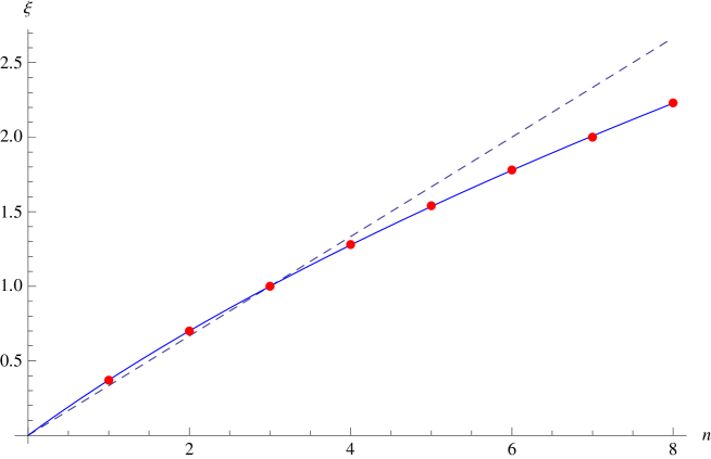
Figure 1: Fit of (5) (blue) to experimental data Benzi (Table 2). The dashed line represents Kolmogorov scaling. The best fit value of the free parameter $\gamma^{2}$ is about 0.161. The error on the data is about $\pm 1$ percent.

Next, we consider the numerical results for low order structure function exponents and non-integer $n$ given in Chen . The numerical data is consistent with experiment at Reynolds number $10^{4}$. For this data, the fitted value of $\gamma^{2}$ is about 0.159 and in Figure 2 we again see excellent agreement.

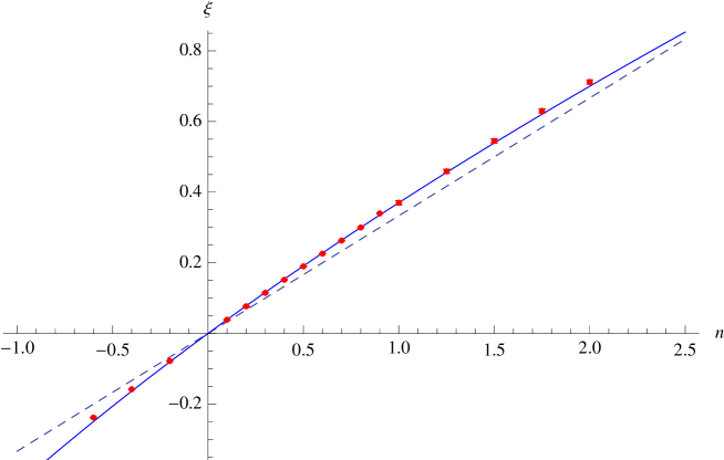
Figure 2: Fit of (5) (blue) to numerical data of low moments Chen (red). The dashed line represents Kolmogorov scaling. The best fit value of the free parameter $\gamma^{2}$ is about 0.159.

Note that if our conjectured relation between the random measure and the local energy dissipation field is correct, one can determine $\gamma^{2}$ independently by measuring the scaling exponent of the two point function, $\langle\epsilon(x)\epsilon(0)\rangle\sim x^{-\gamma^{2}}$. This value has been found to be $\approx 0.2$, which in our formula is still consistent with the data.

I.5.3 Four Space Dimensions

In four space dimensions, numerical simulations of the Navier-Stokes equations were performed in Gotoh2007 . The authors found an increase in intermittency, i.e. $\xi^{(4)}_{n}>\xi^{(3)}_{n}$ for $n<3$, while $\xi^{(4)}_{n}<\xi^{(3)}_{n}$ for $n>3$. We took the data for the structure function exponents in 4d given in Gotoh2007 and performed a fit to (5). This is shown in Figure 3. Although taken at a relatively low Reynolds number, the results are in agreement with a simple increase in the $\gamma^{2}$ parameter in our formula (5). The value of $\gamma^{2}$ in four space dimensions is fitted to about 0.278. Note that their numerical data for same simulation in three space dimensions predicts $\gamma^{2}$ about 0.188, which is higher than the experimental data above. This could be related to the relatively low Reynolds numbers involved.

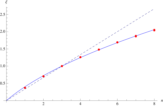
Figure 3: Fit of (5) to the 4d exponents given in Gotoh2007 . The solid line is the 4d fit with $\gamma^{2}$ about 0.278.

I.5.4 Intermittency and the Large $d$ Limit

In order to observe intermittency one has to study the short distance statistical properties of the fluid flow. There are various measures for intermittency, such as $F_{n}(r)=\frac{S_{n}(r)}{S_{2}(r)^{\frac{n}{2}}},~{}~{}~{}n\geq 3$. $F_{n}(r)$ are expected to grow as a power-law in the limit $r\rightarrow 0$, while staying in the inertial range of scales.

We can analyze the properties of $F_{n}(r)$ using (11). They scale as $\sim r^{\alpha}$, where $\alpha$ is a decreasing function of $\gamma$. In the limit $\gamma\rightarrow 0$ one has $\alpha\rightarrow 0$ and no intermittency, while as $\gamma\rightarrow\infty$ we get the maximal intermittency $\alpha=\frac{2-n}{2}$. Numerically, one sees in Gotoh2007 a clear growth of $F_{n}(r),n\geq 4$ in the limit $r\rightarrow 0$, when as we increase the number of space dimensions in the simulation. The data is not accurate enough to observe the growth when $n=3$.

Another exponent that is used to quantify the intermittency is

$$\mu=2-\xi_{6}\ .$$ (17)

Experimentally in three space dimensions it has been measured in the range $0.2$ to $0.25$. Using (11) with $\gamma^{2}=0.161$ we get $\mu=0.222$. Expanding around $\gamma=0$ ($d=2$) we have $\mu=2\gamma^{2}+o(\gamma^{4})$, while expanding around infinite $\gamma$ we have $\mu=1-\frac{1}{\gamma^{2}}+o(\frac{1}{\gamma^{4}})$.

In Falkovich:2009mb , (also see Gotoh2007 ) it was conjectured that in the limit of infinite $d$ all the exponents $\xi_{n}$ approach the same value, one, as in Burgers turbulence Burgers . With our formula (5) this means that $\gamma$ goes to infinity in the limit of infinite $d$, and therefore $\xi_{n}=1$ for any $n$. This suggests the interesting possibility of having a systematic $\frac{1}{d}$ expansion (12).

II Passive Scalar Turbulence

It is natural to ask whether our proposed exact formula for the scaling exponents of incompressible fluid turbulence is applicable for other systems that exhibit turbulent structure. In the following we will consider the Kraichnan model for passive scalar advection by a random Gaussian field of velocities $v^{i}$, which is white-in-time passive1 ; passive2 . The statistics of the velocities is determined by a zero mean $v^{i}(t,\vec{r})=0$, and by the covariance

$$\langle v^{i}(t,\vec{r})v^{i}(t,\vec{r}^{\prime})\rangle=\delta(t-t^{\prime})D^{ij}(\vec{r},\vec{r}^{\prime})\ .$$ (18)

In the inertial range $D^{ij}(\vec{r})-D^{ij}(0)\sim|\vec{r}|^{\zeta}$, where $\zeta$ takes values between 0 and 2.

Examples of passive scalar systems are smoke in the air, salinity in the water and temperature when one can neglect thermal convection. The evolution equation describes a passively-advected scalar field $T$ driven by the velocity field

$$\partial_{t}T+v^{i}\partial_{i}T=\kappa\partial_{jj}T+f\ ,$$ (19)

where $\kappa$ is the molecular diffusivity of $T$ and $f$ is an external force.

One defines the dimensionless Peclet number ${\cal P}_{e}$ as the ratio of the scale of fluctuations of $T$ produced $f$ and the diffusion scale. When ${\cal P}_{e}\gg 1$ there is a scalar turbulence with a scalar cascade and constant flux of $T^{2}$. Similarly to the incompressible fluid turbulence, one is interested here in the stationary statistics and the scaling properties of the scalar structure functions in the inertial range of scales. Define $\delta T(r)=\left(T(\vec{r},t)-T(0,t)\right)$ as the difference between the values of the scalar field at two points separated by a fixed distance $r=|\vec{r}|$. Then,

$$S_{n}(r)=\langle\left(\delta T(r)\right)^{2n}\rangle\sim r^{\xi_{2n}}\ .$$ (20)

Here the scale invariant statistics is Gaussian with $\xi_{2n}=n(2-\zeta)$. We can now attempt to include the intermittency by the random geometry dressing and the KPZ-type equation

$$\xi_{2n}-n(2-\zeta)=\gamma^{2}(d)\xi_{2n}(1-\xi_{2n})\ .$$ (21)

Solving for $\xi_{2n}$ we get

$$\xi_{2n}=\frac{\left((1+\gamma^{2})^{2}+4\gamma^{2}(n(2-\zeta)-1)\right)^{\frac{1}{2}}+\gamma^{2}-1}{2\gamma^{2}}\ .$$ (22)

This formula is similar, but not exactly the one proposed by Kraichnan passive2 . In the limit $n\rightarrow\infty$ for fixed $\gamma$, we have $\xi_{2n}$ growing as $\sqrt{n}$. This is not the expected behaviour, rather $\xi_{2n}$ should approach a constant. This is due to presence of solutions with fronts and shock behaviour, which seems to be characteristic of compressible fluid systems passive . While the KPZ formula does not apply to the passive scalar, it is possible that intermittency in this case ultimately can be described by other, more general types of random geometry, e.g. via the formula (10) above.

III Black Hole Horizon Dynamics

In the following we will briefly review the relation between fluid flows and black hole horizon geometry (for a review, see Eling:2010vr and references therein), that inspired our proposal to incorporate the intermittency at the inertial range of scales by a gravitational dressing using a random geometry. Consider the Einstein equations with a negative cosmological constant $\Lambda$ in $(d+2)$ space-time dimensions

$$E_{AB}\equiv R_{AB}-\frac{1}{2}g_{AB}R+\Lambda g_{AB}=0,~{}~{}~{}~{}A,B=0,...,d+1\ ,$$ (23)

where $g_{AB}$ is the Lorentzian metric, $R_{AB}$ the Ricci curvature and $R=g^{AB}R_{AB}$ the Ricci scalar. Black holes are a classical solution of Einstein equations (23), and their hallmark is the existence of a horizon $H$. For example, a black hole solution to the Einstein equations has the form

$$ds^{2}=g_{AB}dX^{A}dX^{B}=-r^{2}f(r)dt^{2}+2dtdr+r^{2}\sum^{d}_{i=1}dx_{i}dx^{i}\ ,$$ (24)

where the coordinates are $X^{A}=(t,r,x^{i})$. The function $f(r)=1-(\frac{4\pi T}{(d+1)r})^{d+1}$. The horizon is defined as the surface where $f(r)$ vanishes. It is a $(d+1)$-dimensional null hypersurface, forming a causal boundary preventing any light and particles that cross it from returning. Hence, it effectively introduces dissipation. One can associate with the black hole horizon a temperature $T$ (appearing in $f(r)$), and an entropy proportional to its cross-sectional area $A$. In Planck units $\hbar=G_{N}=c=1$, the relation between the area and the entropy is $S_{BH}=\frac{A}{4}$. This structure is called black hole thermodynamics.

Black hole hydrodynamics is a generalization of black hole thermodynamics, similar to the generalization of field theory thermodynamics to hydrodynamics. While black hole thermodynamics quantifies the thermal equilibrium situation, black hole hydrodynamics describes slow derivations from equilibrium. In particular, one can allow the black hole temperature to be a slowly varying function $T(t,x^{i})=const.(1+p(t,x^{i}))$, and consider black hole itself to be moving at velocity $v^{i}(t,x)$ with respect to some rest frame. The perturbed solution to the Einstein equations in this setting will yield a slowly evolving curved geometry, with the gravity variables providing a geometrical framework for studying the dynamics of fluids. This can be made precise in the context of a holographic correspondence, where the fluid system lives on a $(d+1)$ dimensional surface of $r=const.$ in the $(d+2)$ dimensional bulk solution.

The motion of fluids translates to the evolution of the black hole horizon, and the fluid variables to its geometrical data. The normal vector ${\bf n}$ to the horizon $H$ satisfies $g_{AB}n^{A}n^{B}=0$. The horizon hypersurface is defined by $r=r_{H}=const.$ and we have

$$n^{r}=0,~{}~{}~{}~{}n^{t}=1,~{}~{}~{}~{}n^{i}=v^{i}\ .$$ (25)

Thus there is a geometrical representation of the fluid velocity in terms of the normal to the black hole horizon hypersurface. As we perturb the black hole and get it out of equilibrium, the horizon location changes, and up to an overall constant can be parametrized by $r_{H}\sim 1+p(t,x)$. The variable $p(t,x)$ quantifies the deviation from equilibrium and is identified as the fluid pressure. The deviation of the horizon area measure from equilibrium is parametrized by the pressure. One gets that the horizon area measure $\sqrt{\gamma}$ scales like $dp(t,x^{i})$, where $d$ is the number of space dimensions.

The set of the Einstein equations projected on the horizon

$$E_{AB}n^{A}=0\ ,$$ (26)

describe the evolution of the perturbed horizon geometry, and are equivalent to the incompressible NS equations (1) Bhattacharyya:2008kq ; Eling:2009pb . Note that since the Einstein equations are relativistic, this amounts to taking a particular non-relativistic scaling limit of the fully relativistic fluid-gravity equations Bhattacharyya:2008jc ; Eling:2009sj . For example, one of the equations enforces the vanishing of the fractional rate of change of horizon area at lowest order and reduces to the incompressibility condition $\partial_{i}v_{i}=0$.

In the gravitational framework, every fluid configuration that solves the incompressible NS equations corresponds to a particular dual bulk solution and corresponding horizon hypersurface geometry. To describe forced turbulence holographically, one can introduce a background matter term $T_{AB}$ into the Einstein field equations (23) Bhattacharyya:2008ji . This can be used to model the large scale random force pumping energy into the fluid. The energy injected by the pumping ultimately falls into the black hole, where it is dissipated as heat. In the turbulent inertial range, the pressure and velocity are stochastic fields, implying that the dual horizon geometry and measure itself are also random. Therefore, the statistical properties of the random horizon hypersurface (characterized by a sum over surfaces) may encode the universal statistical structure of turbulence. At the horizon, the energy dissipation is related to the flux of matter across the surface, $\int_{\Sigma}T_{AB}n^{A}n^{B}d\Sigma$ Adams:2012pj . Since the horizon itself is random, we were inspired to introduce the random measure in order to quantify the intermittency effects.

IV Discussion

We proposed an analytical formula for the scaling exponents of inertial range incompressible fluid turbulence in any number of space dimensions $d\geq 2$. The idea is that intermittency can be taken into account by a novel gravitational dressing of the scale invariant Kolmogorov spectrum. Mathematically, the coupling to a random geometry with a random measure based on a log correlated field, maps the fractal structure of the scaling exponents to a multifractal one.

There is one parameter that depends on the number of dimensions that we denoted by $\gamma(d)$. It can be deduced knowing one moment, for instance the energy spectrum. With this knowledge one can make infinite number of predictions.

Our formula passes the standard analytical consistency checks, such as the convexity inequality and the absence of a supersonic mode. Its predictions agree with experimental and numerical data in two, three and four space dimensions. The main challenge is to identify the origin of the random geometry in a more precise way and determine analytically the function $\gamma(d)$. We expect the holographic framework that inspired our formula - the relation between fluid dynamics and black hole horizon geometry - to provide a clean calculational scheme. One may also try to calculate $\gamma$ using some physical models for the anomalous scaling, such as contributions from vortex filaments She:1994zz , or statistical conservation laws passive .

While equilibrium statistics is characterized by the Gibbs measure, there is yet no analog of this for non-equilibrium steady state statistics. We speculate that there is a general principle that allows us to consider the steady state statistics of out of equilibrium systems as a gravitationally dressed scale invariant one. If correct, this will shed much light on out of equilibrium dynamics.

Finally, it will be interesting to use the gravitational dressing to study the intermittency effects on the anomalous scaling of the transverse structure functions and multipoint correlation functions. Also, our proposed formula is valid for the inertial range of scales, and most likely does not incorporate statistical signatures of the dissipation range of scales. It is of interest to know whether the latter can be parametrized by a random geometry, since after all the Reynolds number is finite in nature.

References

- (1) U. Frisch, Turbulence: The Legacy of A. N. Kolmogorov, Cambridge University Press (1995).
- (2) A. N. Kolmogorov, Dokl. Akad. Nauk. SSSR 30, 9 (1941); 32, 16 (1941), reproduced in Proc. R. Soc. London, Ser. A 434 9 (1991).
- (3) A. N. Kolmogorov, “A refinement of previous hypotheses concerning the local structure of turbulence in a viscous incompressible fluid at high Reynolds number,” J. Fluid Mech. 13 (1962) 82.
- (4) A. M. Obukhov,“Some specific features of atmospheric turbulence,” J. Fluid Mech. 13 77 (1962).
- (5) B. B. Mandelbrot, “A possible refinement of the lognormal hypothesis concerning the distribution of energy in intermittent turbulence,” in Statistical Models and Turbulence, La Jolla, CA, Lecture Notes in Phys. no. 12, Springer, 333 (1972); “Intermittent turbulence in self-similar cascades, divergence of high moments and dimension of the carrier,” J. Fluid Mech. 62 331 (1974).
- (6) R. Rhodes and V. Vargas, ”Gaussian multiplicative chaos and applications: a review”, arXiv:1305.6221.
- (7) C. Eling, I. Fouxon and Y. Oz, “Gravity and a Geometrization of Turbulence: An Intriguing Correspondence,” Contemporary Physics 52, 43 (2011), [arXiv:1004.2632 [hep-th]].
- (8) V. G. Knizhnik, A. M. Polyakov and A. B. Zamolodchikov, “Fractal Structure of 2D Quantum Gravity,” Mod. Phys. Lett. A 3, 819 (1988).
- (9) R.H. Kraichnan, “Small-scale structure of a scalar field convected by turbulence,” Phys. Fluids 11, 945 (1968).
- (10) R.H. Kraichnan, ”Anomalous scaling of a randomly advected passive scalar”, Phys. Rev. Lett. 72, 1016 (1994).
- (11) I. Benjamini and O. Schramm, ”KPZ in one dimensional random geometry of multiplicative cascades” Comm. Math. Phys. 289 (2), 653 (2008), [arxiv:0806.1347].
- (12) I. Bailleul, ”KPZ in a multidimensional random geometry of multiplicative cascades”, arXiv:1104.3085.
- (13) G. Falkovich, I. Fouxon and Y. Oz, “New relations for correlation functions in Navier-Stokes turbulence,” J. Fluid Mech. 644 (2010) 465; [arXiv:0909.3404 [nlin.CD]].
- (14) R. Benzi, S. Ciliberto, C. Baudet, G. Ruiz Chavarria,“On the scaling of three-dimensional homogeneous and isotropic turbulence,” Physica D 80, 385 (1995).
- (15) T. Gotoh, D. Fukayama, T. Nakano, “Velocity field statistics in homogeneous steady turbulence obtained using a high-resolution direct numerical simulation,” Phys. Fluids 14, 1065 (2002).
- (16) S. Y. Chen, B. Dhruva, S. Kurien, K. R. Sreenivasan and M. A. Taylor, “Anomalous scaling of low-order structure functions of turbulent velocity,” J. Fluid Mech. 553, 183 (2005).
- (17) T. Gotoh, Y. Watanabe, Y. Shiga, T. Nakano, and E. Suzuki, ”Statistical properties of four-dimensional turbulence”, Phys. Rev. E 75, 016310 (2007).
- (18) J. M. Burgers, The Nonlinear Diffusion Equation: Asymptotic Solutions and Statistical Problems (Springer, 1974); U. Frisch and J. Bec, “Burgulence” in New Trends in Turbulence, ed. M. Lesieur, A. Yaglom and F. David (Springer, Berlin, 2000).
- (19) G. Falkovich, K. Gawedzki, M. Vergassola, ”Particles and fields in fluid turbulence”, Rev. Mod. Phys. 73(4), 913-75 (2001), [arXiv:cond-mat/0105199].
- (20) C. Eling, I. Fouxon and Y. Oz, “The Incompressible Navier-Stokes Equations From Membrane Dynamics,” Phys. Lett. B 680, 496 (2009) [arXiv:0905.3638 [hep-th]].
- (21) S. Bhattacharyya, S. Minwalla and S. R. Wadia, “The Incompressible Non-Relativistic Navier-Stokes Equation from Gravity,” JHEP 0908 (2009) 059. [arXiv:0810.1545 [hep-th]].
- (22) S. Bhattacharyya, V. E. Hubeny, S. Minwalla and M. Rangamani, “Nonlinear Fluid Dynamics from Gravity,” JHEP 0802, 045 (2008) [arXiv:0712.2456 [hep-th]].
- (23) C. Eling and Y. Oz, “Relativistic CFT Hydrodynamics from the Membrane Paradigm,” JHEP 1002, 069 (2010) [arXiv:0906.4999 [hep-th]].
- (24) S. Bhattacharyya, R. Loganayagam, S. Minwalla, S. Nampuri, S. P. Trivedi and S. R. Wadia, “Forced Fluid Dynamics from Gravity,” JHEP 0902, 018 (2009) [arXiv:0806.0006 [hep-th]].
- (25) A. Adams, P. M. Chesler and H. Liu, “Holographic Vortex Liquids and Superfluid Turbulence,” Science 341, 368 (2013) [arXiv:1212.0281 [hep-th]].
- (26) Z. S. She and E. Leveque, “Universal scaling laws in fully developed turbulence,” Phys. Rev. Lett. 72, 336 (1994).