Off-Policy Reward Shaping with Ensembles

Abstract

Potential-based reward shaping (PBRS) is an effective and popular technique to speed up reinforcement learning by leveraging domain knowledge. While PBRS is proven to always preserve optimal policies, its effect on learning speed is determined by the quality of its potential function, which, in turn, depends on both the underlying heuristic and the scale. Knowing which heuristic will prove effective requires testing the options beforehand, and determining the appropriate scale requires tuning, both of which introduce additional sample complexity.

We formulate a PBRS framework that improves learning speed, but does not incur extra sample complexity. For this, we propose to simultaneously learn an ensemble of policies, shaped w.r.t. many heuristics and on a range of scales. The target policy is then obtained by voting. The ensemble needs to be able to efficiently and reliably learn off-policy: requirements fulfilled by the recent Horde architecture, which we take as our basis. We demonstrate empirically that (1) our ensemble policy outperforms both the base policy, and its single-heuristic components, and (2) an ensemble over a general range of scales performs at least as well as one with optimally tuned components.

1 Introduction

The powerful ability of reinforcement learning (RL) sutton-barto98 to find optimal policies tabula rasa, is also the source of its main weakness: infeasibly long running times. As the problems RL tackles get larger, it becomes increasingly important to leverage all possible knowledge about the domain at hand. One paradigm to inject such knowledge into the reinforcement learning problem is potential-based reward shaping (PBRS) ng99 . Aside from repeatedly demonstrated efficacy in increasing learning speed asmuth2008potential ; devlin11 ; brys2014combining ; snelshimonshaping , the principal strength of PBRS lies in its ability to preserve optimal policies. Moreover, it is the only reward shaping scheme that is guaranteed to do so ng99 . At the heart of PBRS methods lies the potential function. Intuitively, it expresses the “desirability” of a state, defining the shaping reward on a transition to be the difference in potentials of the transitioning states. States may be desirable by many criteria. The pursuit of designing a potential function that accurately encapsulates the “true” desirability is meaningless, as it would solve the task at hand ng99 , and remove the need for learning altogether. However, one can usually suggest many simple heuristic criteria that improve performance in different situations. Choosing the most effective heuristic amongst them without a test comparison, is typically infeasible, and carrying out such a comparison implies added sample complexity, that may be unaffordable. Moreover, heuristics may contribute complementary knowledge that cannot be leveraged in isolation brys2014combining .

The choice of a heuristic is merely one of the two deciding factors for the performance of a potential function. The other (and one that is even less intuitive) is scaling. An effective heuristic with a sub-optimal scaling factor may make no difference at all, if the factor is too small, or dominate the base reward and distract the learner, if the factor is too large. Typically, one is required to tune the scaling factor beforehand, which requires extra environment samples, and is infeasible in realistic problems.

We wish to devise a PBRS framework that is capable of improving learning speed, without introducing extra sample complexity. To this end, rather than learn a single policy shaped with the most effective heuristic on its optimal scale, we propose to maintain an ensemble of policies that all learn from the same experience, but are shaped w.r.t. different heuristics and different scaling factors. The deployment of our ensemble thus does not require any additional environment samples, and frees the designer up to benefit from PBRS, equipped only with a set of intuitive heuristic rules, with no necessary knowledge of their performance and value magnitudes.

Because (for the purpose of not requiring extra environment samples), all member-policies learn to maximize different reward functions from the same experience, the learning needs to be reliable off-policy. Because the introduced computational complexity (for each of the additional member-policies) amounts to that of the off-policy learner, we wish for the learning to be as efficient as possible. The recently introduced Horde architecture sutton09 is well-suited to be the basis of our ensemble, due to its general off-policy convergence guarantees and computational efficiency. In contrast to the previous uses of Horde pilarski2013 , we exploit its power to learn a single task, but from multiple viewpoints.

The convergence guarantees of Horde require a latent learning scenario maei2010 , i.e. one of (off-policy) learning under a fixed (or slowly changing) behavior policy. This scenario is particularly relevant to real-world applications, where failure is highly penalized and the usual trial-and-error tactic is implausible, e.g. robotic setups. One could imagine the agent following a safe exploratory policy, while learning the target control policy, and only executing the target policy after it is learnt. That is the scenario we focus on in this paper. Note that the conventional interpretation of PBRS to steer exploration grzes2010diss , does not apply here, as the behavior is unaffected by the target policy, and is kept fixed. This work (and its precursor harutyunyan2014ecai ) provides, to our knowledge, the first validation of PBRS effective in such a latent setting.

Our contribution is two-fold: (1) we formulate and empirically validate a PBRS framework as a policy ensemble, that is capable of increasing learning speed without adding extra sample complexity, and that does so with general convergence guarantees. Specifically, we demonstrate how such an ensemble can be used to lift the problems of both the choice of the potential function and its scaling, thus removing the need of behind-the-scenes tuning necessary before deployment; and (2) we validate PBRS to be effective in a latent off-policy setting, in which it cannot steer the exploration strategy.

In the following section we give an overview of the preliminaries. Section 3 motivates our approach further, while Section 4 describes the proposed architecture and the voting techniques used to obtain the target ensemble policy. Section 5 presents empirical results in two classical benchmarks, and Section 6 concludes.

2 Background

We assume the usual RL framework sutton-barto98 , in which the agent interacts with its (typically) Markovian environment at discrete time steps $t=1,2,\ldots$. Formally, a Markov Decision Process (MDP) puterman94 is a tuple ${\cal M}=\langle{\cal S},{\cal A},\gamma,{\cal T},R\rangle$, where: $\cal S$ is a set of states, $\cal A$ is a set of actions, $\gamma\in[0,1]$ is the discounting factor, ${\cal T}=\{P_{sa}(\cdot)|s\in{\cal S},a\in{\cal A}\}$ are the next state transition probabilities with $P_{sa}(s^{\prime})$ specifying the probability of state $s^{\prime}$ occuring upon taking action $a$ from state $s$, $R:{\cal S}\times{\cal A}\times{\cal S}\rightarrow{\mathbb{R}}$ is the reward function with $R(s,a,s^{\prime})$ giving the expected value of the reward that will be received when $a$ is taken in state $s$, and $r_{t+1}$ denoting the component of $R$ at time $t$.

A (stochastic) Markovian policy $\pi:{\cal S}\times{\cal A}\rightarrow[0,1]$ is a probability distribution over actions at each state, s.t. $\pi(s,a)$ gives the probability of action $a$ being taken from state $s$ under policy $\pi$. In the deterministic case, we will take $\pi(s)=a$ to mean $\pi(s,a)=1$.

Value-based methods encode policies through value functions, which denote expected cumulative reward obtained while following the policy. We focus on state-action value functions. In a discounted setting:

$$Q^{\pi}(s,a)=\mathbb{E}_{{\cal T},\pi}\Big{[}\sum\limits_{t=0}^{\infty}\gamma^{t}r_{t+1}|s_{0}=s,a_{0}=a\Big{]}$$ (1)

An action $a^{*}$ is greedy in a state $s$, if it is the action of maximum value in $s$. A (deterministic) policy is greedy, if it picks the greedy action in each state:

$$\pi(s)=\operatorname*{arg\,max}_{a}Q^{\pi}(s,a),\forall s\in{\cal S}$$ (2)

A policy $\pi^{*}$ is optimal if its value is largest:

$$Q^{*}(s,a)=\sup_{\pi}Q^{\pi}(s,a),\forall s\in{\cal S},\forall a\in{\cal A}$$

The learning is on-policy if the behavior policy $\pi_{b}$ that the agent is following is the same as the target policy $\pi$ that the agent is evaluating. Otherwise, it is off-policy. Given $\pi_{b}$, the values of the optimal greedy policy can be learned incrementally through the following Q-learning watkins1992 update:

$$Q_{t+1}(s_{t},a_{t})=Q_{t}(s_{t},a_{t})+\alpha_{t}\delta_{t}$$ (3)

$$\delta_{t}=r_{t}+\gamma\max\limits_{a^{*}\in{\cal A}}Q_{t}(s_{t+1},a^{*})-Q_{t}(s_{t},a_{t})$$ (4)

where $Q_{t}$ is an estimate of $Q^{\pi}$ at time $t$, $\alpha_{t}\in(0,1)$ is the learning rate at time $t$, $a_{t}$ is chosen according to $\pi_{b}$, $\delta_{t}$ is the temporal-difference (TD) error of the transition. $s_{t+1}$ is drawn according to ${\cal T}$, given $s_{t}$ and $a_{t}$, and $a^{*}$ is the greedy action w.r.t. $Q_{t}$ in $s_{t+1}$ Given tabular representation, this process is shown to converge to the correct value estimates (the TD-fixpoint) in the limit under standard approximation conditions jaakkola1994convergence .

When the state or action spaces are too large, or continuous, tabular representations do not suffice and one needs to use function approximation (FA). The state (or state-action) space is then represented through a set of features $\phi$, and the algorithms learn the value of a parameter vector $\theta$. In the (common) linear case:

$$Q_{t}(s,a)=\theta_{t}^{T}\phi_{s,a},\forall s\in{\cal S},\forall a\in{\cal A}$$ (5)

and Eq. (3) becomes:

$$\theta_{t+1}=\theta_{t}+\alpha_{t}\delta_{t}\phi_{t},$$ (6)

where we slightly abuse notation by letting $\phi_{t}$ denote the state-action features $\phi_{s_{t},a_{t}}$, and $\delta_{t}$ is still computed according to Eq. (4).

In the next two subsections we present the core ingredients to our approach.

2.1 Horde

FA is known to cause off-policy bootstrapping methods (such as Q-learning) to diverge even on simple problems baird95 ; Tsitsiklis97ananalysis . The family of gradient temporal difference (GTD) methods provides a solution for this issue, and guarantees off-policy convergence under FA, given a fixed (or slowly changing behavior) sutton09 . Previously, similar guarantees were provided only by second-order batch methods (e.g. LSTD Bradtke96linearleast-squares ), unsuitable for online learning. GTD methods are the first to maintain these guarantees, while maintaining the (time and space) complexity linear in the size of the state space. Note that linearity is a lower bound on what is achievable, because it is required to simply store and access the learning vectors. As a consequence, GTD methods scale well to the number of value functions (policies) learnt modayil2012acquiring , and due to the inherent off-policy setting, can do so from a single stream of environment interactions (or experience). Sutton et al. sutton11 formalize this idea in a framework of parallel off-policy learners, called Horde. They demonstrate Horde to be able to learn thousands of predictive and goal-oriented value functions in real-time from a single unsupervised stream of sensorimotor experience. There have been further successful applications of Horde in realistic robotic setups pilarski2013 .

On the technical level, GTD methods are based on the idea of performing gradient descent on a reformulated objective function, which ensures convergence to the projected TD-fixpoint, by introducing a gradient bias into the TD-update sutton09 . Mechanistically, it requires maintaining and learning a second set of weights $w$, along with $\theta$, and performing the following updates:

$$\theta_{t+1} = \theta_{t}+\alpha_{t}\delta_{t}\phi_{t}-\alpha\gamma\phi^{\prime}_{t}(\phi_{t}^{T}w_{t})$$ (7)

$$w_{t+1} = w_{t}+\beta_{t}(\delta_{t}-\phi_{t}^{T}w_{t})\phi_{t}$$ (8)

where $\delta_{t}$ is still computed with Eq. (4), and $\phi^{\prime}_{t}$ is the feature vector of the next state and action. This is a simpler form of the GTD-update, namely that of TDC sutton09 . GQ($\lambda$) maei2010gq augments this update with eligibility traces.

Convergence is one of the two theoretical hurdles with off-policy learning under FA. The other has to do with the quality of solutions under off-policy sampling, which may, in general, fall far from optimum, even when the approximator can represent the true value function well. In, to our knowledge, the only work that addresses this issue, Kolter kolter2011fixed gives a way of constraining the solution space to achieve stronger qualitative guarantees, but his algorithm has quadratic complexity and thus is not scalable. Since scalability is crucial in our framework, Horde remains the only plausible convergent architecture available.

2.2 Reward Shaping

Reward shaping augments the true reward signal $R$ with an additional shaping reward $F$, provided by the designer. The shaping reward is intended to guide the agent, when the environmental rewards are sparse or uninformative, in order to speed up learning. In its most general form:

$$R^{\prime}=R+F$$ (9)

Because tasks are identified by their reward function, modifying the reward function needs to be done with care, in order to not alter the task, or else reward shaping can slow down or even prevent finding the optimal policy Randløv98 . Ng et al. ng99 show that grounding the shaping rewards in state potentials is both necessary and sufficient for ensuring preservation of the (optimal) policies of the original MDP. Potential-based reward shaping (PBRS) maintains a potential function $\Phi:S\rightarrow{\mathbb{R}}$, and defines the auxiliary reward function $F$ as:

$$F(s,a,s^{\prime})=\gamma\Phi(s^{\prime})-\Phi(s)$$ (10)

where $\gamma$ is the discounting factor of the MDP. We refer to the rewards, value functions and policies, augmented with shaping rewards as shaped. Shaped policies converge to the same (optimal) policies as the base learner, but differ during the learning process.

3 A Horde of Shapings

The key insight in ensemble learning is that the strength of an ensemble lies in the diversity its components contribute Krogh95neuralnetwork . In the RL context, this diversity can be expressed through several aspects, related to dimensions of the learning process: (1) diversity of experience, (2) diversity of algorithms and (3) diversity of reward signals. Diversity of experience naturally implies high sample complexity, and assumes either a multi-agent setup, or learning in stages. Diversity of algorithms (given the same experience) is computationally costly, as it requires separate representations, and one needs to be particular about the choice of algorithms due to convergence considerations. In the context of our aim of increasing learning speed, without introducing complexity elsewhere, we focus on the latter aspect of diversity: diversity of reward signals.

PBRS is an elegant and theoretically attractive approach to introducing diversity into the reward function, by drawing from the available domain knowledge. Such knowledge can often be described as a set of simple heuristics. Combining the corresponding potentials beforehand naïvely (e.g. with linear scalarization) may result in information loss, when the heuristics counterweigh each other, and introduce further scaling issues, since the relative magnitudes of the potential functions may differ. Maintaining the shapings separately has recently been shown to be a more robust and effective approach brys2014combining . Under the requirements of convergence and efficiency, maintaining such an ensemble of policies learning in parallel and shaped with different potentials, is only possible via the Horde architecture, which is the approach we take in this paper. Thus, the proposed ensemble is the first of its kind to possess general convergence guarantees.

Horde’s demonstrated ability to learn thousands of policies in parallel in real time sutton11 ; modayil2012acquiring allows to consider large ensembles, at little computational cost. While defining thousands of distinct heuristics is rarely sensible, each heuristic may be learnt on many different scaling factors. This not only frees one from having to tune the scaling factor a priori (one of the issues we focus on in this paper), but potentially allows for automatically dynamic scaling, corresponding to state-dependent shaping magnitudes.

Shaping Off-Policy

The effects of PBRS on the learning process are usually considered to lie in the guidance of exploration during learning grzes2010diss ; marthi2007 ; ng99 . Laud and DeJong laud03 formalize this by showing that the difficulty of learning is most dependent on the reward horizon, a measure of the number of decisions a learning agent must make before experiencing accurate feedback, and that reward shaping artificially reduces this horizon. In our latent setting we assume no control over the agent’s behavior. The performance benefits then can be explained by faster knowledge propagation through the TD updates, which we now observe decoupled from guidance of exploration.

Reward shaping in such off-policy settings is not well studied or understood, and these effects are of independent interest.

4 Architecture

We are now ready to describe the architecture of our ensemble (Fig. 1).We maintain our Horde of shapings as a set $\cal D$ of Greedy-GQ($\lambda$)-learners maei2010gq . Given a set of potential functions ${\bf\Phi}=\{\Phi_{1},\ldots\Phi_{\ell}\}$ a range of scaling factors ${\bf c}^{i}=\langle c^{i}_{1},\ldots c^{i}_{k_{i}}\rangle$ for each $\Phi_{i}$, and the base reward function $R$, the ensemble reward function is a vector:

$${\bf R}=R+\langle F_{c^{1}_{1}}^{\Phi_{1}},F_{c^{1}_{2}}^{\Phi_{1}},\ldots,F_{c^{\ell}_{k_{\ell}}}^{\Phi_{\ell}}\rangle$$ (11)

where $F^{\Phi_{i}}_{c^{i}_{j}}$ is the potential-based shaping reward given by Eq. (10) w.r.t. the potential function $\Phi_{i}$ and scaled with the factor $c^{i}_{j}$. For notational clarity, we will take $F^{i}_{j}$ to mean $F^{\Phi_{i}}_{c^{i}_{j}}$ (i.e. the shaping w.r.t. to the $i$-th potential function on the $j$-th scaling factor), and $R^{i}_{j}=R+F^{i}_{j}$. We allow the ensemble the option to include the base learner.

We adopt the terminology of Sutton et al. sutton11 , and refer to individual agents within Horde as demons. Each demon $d^{i}_{j}$ learns a greedy policy $\pi^{i}_{j}$ w.r.t. its reward $R^{i}_{j}$. Recall that our latent setting implies that the learning is guided by a fixed behavior policy $\pi_{b}$, with $\pi^{i}_{j}$ all learning in parallel from the experience generated by $\pi_{b}$. Because each policy $\pi^{i}_{j}$ is available separately at each step, an ensemble policy can be devised by collecting votes on action preferences from all demons $d^{i}_{j}$. The ensemble is also latent, and not executed until the learning has ended. Note that because PBRS preserves all of the optimal policies from the original problem ng99 , the ensemble policy does too.

In this paper we have considered two voting schemes: majority voting and rank voting, which are elaborated below. The architecture is certainly not limited to these choices.

4.1 Ensemble Policy

To the best of our knowledge, both voting methods were first used in the context of RL agents by Wiering and Van Hasselt wiering08 . In both methods, each demon $d$ casts a vote $v_{d}:S\times A\rightarrow{\mathbb{N}}^{0}$, s.t. $v_{d}(s,a)$ is the preference value of action $a$ in state $s$. The voting scheme then is defined for policies, rather than value functions, which mitigates the magnitude bias. The ensemble policy acts greedily (with ties broken randomly) w.r.t. the cumulative preference values $P$:

$$P(s_{t},a)=\sum\limits_{d\in\cal D}v_{d}(s_{t},a),\forall a\in A$$ (12)

The voting scheme determines the manner in which $v_{d}$ are assigned.

Majority voting

Each demon $d$ casts a vote of 1 for its most preferred action, and a vote of 0 for the others. I.e.:

$$v_{d}(s,a)=\begin{cases}1&\mbox{if }Q(s,a)=\max\limits_{a^{*}}Q(s,a^{*})\\ 0&\mbox{otherwise.}\end{cases}$$ (13)

Rank voting

Each demon greedily ranks its $n$ actions, from $n-1$ for its most, to $0$ for its least preferred actions. We slightly modify the formulation from wiering08 , by ranking Q-values, instead of policy probabilities. I.e. $v_{d}(s,a)>v_{d}(s,a^{\prime})$, if and only if $Q_{d}(s,a)>Q_{d}(s,a^{\prime})$.

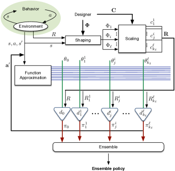
Figure 1: An overview of the Horde architecture used to learn an ensemble of shapings (including the base learner). Vectors are indicated with bold lines. $R^{i}_{j}$ is the reward obtained when applying $\Phi_{i}$ to $R$ and scaling with $c^{i}_{j}$. The blue output of the linear function approximation block are the features of the transition (two state-action pairs), with their intersections with $\theta^{i}_{j}$ representing weights. ${\bf a^{\prime}}$ is a vector of greedy actions at $s^{\prime}$ w.r.t. to each policy $\pi^{i}_{j}$. Note that in this latent settings, all interactions with the environment happen only in the upper left corner.

5 Experiments

We now present the empirical studies that validate the efficacy of our ensemble architecture w.r.t. both the choice of heuristic and the choice of scale. We first consider the scenario of choosing between heuristics, and evaluate an ensemble consisting of shapings with appropriate scaling factors. The experiments show that the ensemble policy performs at least as well as the best heuristic. We then turn to the problem of scaling, and demonstrate that ensembles on both narrow and broad ranges of scales perform at least as well as the one w.r.t. the optimal scaling factors.

We carry out our experiments on two common benchmark problems. In both problems, the behavior policy is a uniform distribution over all actions at each time step. The evaluation is done by interrupting the base learner every $z$ episodes and executing the queried greedy policy once. No learning is allowed during evaluation.

We evaluated the ensembles w.r.t. both voting schemes from Sec. 4.1, and found the (sum) performance to be not significantly different ($p>0.05$), with rank voting performing slightly better. To keep the clarity of focus, below we only present the results for the rank voting scheme, but emphasize that the performance is not conditional on this choice.

5.1 Mountain Car

We begin with the classical benchmark domain of mountain car sutton-barto98 . The task is to drive an underpowered car up a hill. The (continuous) state of the system is composed of the current position (in $[-1.2,0.6]$) and the current velocity (in $[-0.07,0.07]$) of the car. Actions are discrete, a throttle of $\{-1,0,1\}$. The agent starts at the position $-0.5$ and a velocity of $0$, and the goal is at the position $0.6$. The rewards are $-1$ for every time step. An episode ends when the goal is reached, or when 2000 steps have elapsed. The state space is approximated with the standard tile-coding technique sutton-barto98 , using ten tilings of $10\times 10$, with a parameter vector learnt for each action.

In this domain we define three intuitive shaping potentials:

Position

Encourage progress to the right (in the direction of the goal). This potential is flawed by design, since in order to get to the goal, one needs to first move away from it.

$$\Phi_{1}({\bf x})=\bar{x}$$ (14)

Height

Encourage higher positions (potential energy):

$$\Phi_{2}({\bf x})=\bar{h}$$ (15)

Speed

Encourage higher speeds (kinetic energy):

$$\Phi_{3}({\bf x})=|\bar{\dot{x}}|^{2}$$ (16)

Here ${\bf x}=\langle x,\dot{x}\rangle$ is the state (position and velocity), and $\bar{a}$ denotes the normalization of $a$ onto $[0,1]$.

We used $\gamma=0.99$. The learning parameters were tuned w.r.t. the base learner and shared among all demons: $\lambda=0.4,\beta=0.0001,\alpha=0.1$, where $\lambda$ is the trace decay parameter, $\beta$ the step size for the second set of weights $w$ in Greedy-GQ, and $\alpha$ the step size for the main parameter vector $\theta$. We ran 1000 independent runs of 100 episodes each, with evaluation occuring every 5 episodes ($z=5$).

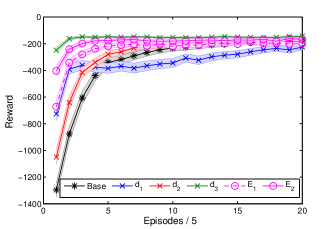
Figure 2: Learning curves of the single shapings and their ensembles in mountain car. $E_{1}$, the ensemble of two comparable shapings, outperforms both of them, whereas $E_{2}$, the ensemble of all three shapings, matches ($p>0.05$) the performance of the (more effective) third shaping $d_{3}$.

5.1.1 Choice of Heuristic

In this experiment we address the question of the choice between heuristics. We thus consider ensembles composed of the demons shaped with the three shaping potential functions $\Phi_{1}$,$\Phi_{2}$ and $\Phi_{3}$, and scaled with factors $c_{1},c_{2},c_{3}$ that have been tuned beforehand. We associate the learner $d_{i}$ with $d^{\Phi_{i}}_{c_{i}}$.

When evaluating the shapings individually, we witness $d_{3}$ to perform best amongst the three. To examine the quality of our ensembles w.r.t. the quality of its components, we consider two scenarios: $E_{1}=\langle d_{1},d_{2}\rangle$ of two demons and $E_{2}=\langle d_{1},d_{2},d_{3}\rangle$ of three demons. This corresponds to having ensemble consisting of two comparable shapings, and an ensemble with one clearly most efficient shaping. Thus, ideally, we would like $E_{1}$ to outperform both $d_{1}$ and $d_{2}$ and $E_{2}$ to at least match the performance of $d_{3}$.

Fig. 2 presents the learning performance of the base agent, the demons $d_{1},d_{2},d_{3}$ shaped with single potentials, and the two ensembles $E_{1}$ and $E_{2}$, mentioned above. We witness the individual shapings alone to aid the learning significantly. $E_{1}$ follows $d_{1}$ at first, when its performance is better, but switches to $d_{2}$, when the performance of $d_{1}$ levels out. This is because $d_{1}$ (as is appropriate with its position shaping) persists on going right in the beginning of an episode, and this strategy, while effective at first, results in a plateau of a higher number of steps. The ensemble policy is able to avoid this by incorporating information from $d_{2}$.

$E_{2}$, the ensemble of all three shapings, begins better than both $d_{1}$ and $d_{2}$, but slightly worse than $d_{3}$, the most effective shaping. It, however, quickly catches up to $d_{3}$, with the overall performance of $E_{2}$ and $d_{3}$ being statistically indistinguishable.

Thus, the performance of the ensembles meets our desiderata: when there is clearly a best component, an ensemble statistically matches it, otherwise it outperforms all of its components.

5.1.2 Choice of Scale

The previous set of experiments assumed access to the best scaling factors $c_{1},c_{2},c_{3}$. In practice obtaining these requires tuning each shaping prior to the use of the ensemble, a scenario we aim to avoid. In this section we demonstrate that ensembles on a range of scales perform at least as well, as those with cherry-picked components.

Namely, we consider two scaling ranges $C_{1}=\langle 20,40,60,80,100\rangle$ and $C_{2}=\langle 1,10,10^{2},10^{3},10^{4}\rangle$, with the first being a reasonably close range to the optimal scales from the previous section, and the second being a general sweep, with no intuition or knowledge of the optimal scale. Before we proceed further, we illustrate the effect a scaling factor can have on the performance of a single shaping. Fig. 3 gives a comparison of the performance of the shaping potential $\Phi_{2}$ over the (reasonable) scaling range $C_{1}$. Even small differences in scale have dramatic effect on the shaping’s performance.

Now let $E_{C_{1}}$ and $E_{C_{2}}$ be the ensembles w.r.t. all three shapings on $C_{1}$ and $C_{2}$, resp., each totaling in 16 demons (including the base learner). We compare $E_{C_{1}}$ and $E_{C_{2}}$ with $E_{2}$ (the ensemble w.r.t. the three shapings with tuned scaling factors, from the first experiment). We illustrate the range of performances of shapings for each scale range, by additionally plotting the average of the runs of each shaping across each scale. I.e. for the range $C_{j}$, and shaping $\Phi_{i}$, at each episode, this is the average of the rewards obtained by the demons $d^{i}_{1}$, $d^{i}_{2}$,$\ldots$,$d^{i}_{|C_{j}|}$ in that episode.

Fig. 4 presents the results. $E_{C_{1}}$ and $E_{C_{2}}$ are both statistically the same ($p>0.05$) as the tuned ensemble $E_{2}$, despite their components having a much wider range of performance.

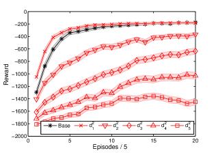
Figure 3: The range of performance of a single shaping w.r.t. different scales in mountain car. Each curve corresponds to the performance of a demon shaped with $\Phi_{2}$, with a scaling factor from the range $C_{1}$.

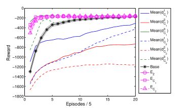
Figure 4: Learning curves of the ensembles over the scale ranges $C_{1}$ and $C_{2}$ in mountain car. The solid and dashed lines (for each of the three shapings) are the mean performance of the demons w.r.t. $C_{1}$ and $C_{2}$, respectively, and are plotted as a reference for the performance of the ensemble components. Note that there is no single demon with this performance. The performances of ensembles $E_{C_{1}}$ and $E_{C_{2}}$ are not significantly different from that of $E_{2}$: the ensemble w.r.t. tuned components.

5.2 Cart-Pole

We now validate our framework on the problem of cart-pole michie:boxes . The task is to balance a pole on top of a moving cart for as long as possible. The (continuous) state $\bf s$ contains the angle $\xi$ and angular velocity $\dot{\xi}$ of the pole, and the position $x$ and velocity $\dot{x}$ of the cart. There are two actions: a small positive and a small negative force applied to the cart. A pole falls if $|\xi|>\frac{\pi}{4}$, which terminates the episode. The track is bounded within $[-4,4]$, but the sides are “soft”; the cart does not crash upon hitting them. The reward function penalizes a pole drop, and is 0 elsewhere. An episode terminates successfully, if the pole was balanced for 1000 steps. The state space is approximated with tile coding, using ten tilings of $10\times 10$ over all 4 dimensions, with a parameter vector learnt for each action.

We define two potential functions, corresponding to the angle and angular speed of the pole.

Angle

Discourage angles far from the equilibrium:

$$\Phi_{1}({\bf s})=-\bar{|\xi|}^{2}$$ (17)

Angular speed

Discourage high speeds (which are likelier to result in dropping the pole):

$$\Phi_{2}({\bf s})=-|\bar{\dot{\xi}}|^{2}$$ (18)

We used $\gamma=0.99$. The learning parameters were tuned w.r.t. the base learner and set to $\lambda=0.7$, $\alpha=0.1$ and $\beta=0.001$. These settings were shared among all demons. We ran 100 independent runs of a 1000 episode each, with evaluation occuring every 50 episodes ($z=50$).

5.2.1 Choice of Heuristic and Scale

In this experiment we evaluate the problems of the choice of the heuristic and its scale jointly. We consider a general scaling range $C=\langle 1,10,10^{2},10^{3},10^{4}\rangle$, and three ensembles: $E^{1}_{C}$ resp. $E^{2}_{C}$ only comprised of the demons shaped w.r.t. $\Phi_{1}$ resp. $\Phi_{2}$ across $C$ (5 demons each), and $E_{C}$ containing all 11 demons (including the base learner). As before, we illustrate the range of performances of shapings across the range of scales by, for each shaping, plotting the average performance of the demons w.r.t. that shaping across the entire scale range. I.e. for the shaping $\Phi_{i}$, at each episode, this is the average of the rewards obtained by the demons $d^{i}_{1}$, $d^{i}_{2}$,$\ldots$,$d^{i}_{|C|}$ in that episode.

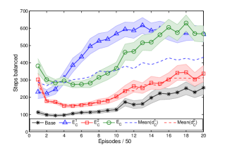
Figure 5: Learning curves for the ensembles $E^{1}_{C}$, $E^{2}_{C}$ and $E_{C}$ in cart-pole. The dashed lines (for each of the two shapings) denote the mean performance of the demons w.r.t. $C$, and plotted as a reference for the performance of the ensemble components. Note that there is no single demon with this performance. The performances of the global ensemble $E_{C}$ follows the (more effective) first shaping, in the end matching the performance of the corresponding ensemble $E^{1}_{C}$.

Fig. 5 shows the results. All ensembles (and ensemble averages) improve over the base learner. The performance of $E^{2}_{C}$, the ensemble over the second shaping, matches that of the average from that ensemble, since all of its components perform similarly. On the other hand, $E^{1}_{C}$, the ensemble over the first shaping, does much better than the corresponding average. The global ensemble $E_{C}$ over all of the demons starts out better than both $E^{1}_{C}$ and $E^{2}_{C}$, then levels at the average performance of the (better) first shaping, and finally matches the performance of $E^{1}_{C}$. The global ensemble $E_{C}$ thus correctly identifies both which shaping to follow: its performance always follows (or is better than) that of the more efficient first shaping (either on average, or the ensemble $E^{1}_{C}$), and on what scales: the final performance of $E_{C}$ matches that of $E^{1}_{C}$, significantly improving over the average across the scale range.

6 Conclusions

In this work we described a novel off-policy PBRS ensemble architecture that is able to improve learning speed in a latent setting, without requiring the extra sample complexity introduced by the steps of tuning the heuristic and its scale, typical to PBRS. We avoid these steps by learning an ensemble of policies w.r.t. many heuristics and scaling factors simultaneously. Our ensemble possesses general convergence guarantees, while staying efficient, as it leverages the recent Horde architecture to learn a single task well. Our experiments validate the use of PBRS in the latent setting, and demonstrate the efficacy of the proposed ensemble. Namely, we show that the ensemble policy over both broad and narrow ranges of scales performs at least as well as the one over a set of optimally pre-tuned components, which in turn performs at least as well as its best component-heuristic.

Future Directions

In this work we have assumed a shared set of parameters between the demons, an immediate extension would be to maintain demons that learn w.r.t. different parameters. This is similar to the approach of Marivate and Littman marivate2013 , who learn to solve many variants of a problem for the best parameter settings in a generalized MDP. In our case the MDP (dynamics) will remain shared, but the individual parameters of the demons will vary.

It would be worthwhile to evaluate the framework w.r.t. different ensemble techniques that induce the target ensemble policy. This would be especially useful in domains where only select scaling factors of select heuristics offer improvement: taking a global majority vote over such an ensemble will likely not be as effective, as trying to determine which subset of demons to consider. One could, e.g., use confidence measures brys2014combining to identify these demons.

Instead of shaping demons with static potential functions, one could consider maintaining a layer of demons that each learn some potential function marthi2007 ; grzes2010 , which are, in turn, fed into the layer of shaped demons who contribute to the ensemble policy. One needs to be realistic about attainability of learning this in time, since as argued by Ng et al. ng99 , the best potential function correlates with the optimal value function $V^{*}$, learning which would solve the base problem itself and render the potentials pointless.

References

- [1] J. Asmuth, M. L. Littman, and R. Zinkov. Potential-based shaping in model-based reinforcement learning. In Proceedings of AAAI, pages 604–609, 2008.
- [2] L. Baird. Residual algorithms: Reinforcement learning with function approximation. In Proceedings of ICML, pages 30–37, 1995.
- [3] S. J. Bradtke, A. G. Barto, and P. Kaelbling. Linear least-squares algorithms for temporal difference learning. In Machine Learning, pages 22–33, 1996.
- [4] T. Brys, A. Nowé, D. Kudenko, and M. E. Taylor. Combining multiple correlated reward shaping signals by measuring confidence. In Proceedings of AAAI, 2014.
- [5] S. Devlin, D. Kudenko, and M. Grzes. An empirical study of potential-based reward shaping and advice in complex, multi-agent systems. Advances in Complex Systems (ACS), 14(02):251–278, 2011.
- [6] M. Grzes. Improving Exploration in Reinforcement Learning through Domain Knowledge and Parameter Analysis. PhD thesis, University of York, 2010.
- [7] M. Grzes and D. Kudenko. Online learning of shaping rewards in reinforcement learning. Neural Networks, 23(4):541 – 550, 2010. Proceedings of ICANN.
- [8] A. Harutyunyan, T. Brys, P. Vrancx, and A. Nowé. Off-policy shaping ensembles in reinforcement learning. In Proceedings of ECAI, pages 1021–1022, 2014.
- [9] T. Jaakkola, M. I. Jordan, and S. P. Singh. On the convergence of stochastic iterative dynamic programming algorithms. Neural computation, 6(6):1185–1201, 1994.
- [10] J. Z. Kolter. The fixed points of off-policy TD. In Advances in Neural Information Processing Systems, pages 2169–2177, 2011.
- [11] A. Krogh and J. Vedelsby. Neural network ensembles, cross validation, and active learning. In Advances in Neural Information Processing Systems, pages 231–238, 1995.
- [12] A. Laud and G. DeJong. The influence of reward on the speed of reinforcement learning: An analysis of shaping. In Proceedings of ICML, 2003.
- [13] H. Maei. Gradient Temporal-Difference Learning Algorithms. PhD thesis, University of Alberta, 2011.
- [14] H. Maei and R. Sutton. GQ(): A general gradient algorithm for temporal-difference prediction learning with eligibility traces. In Proceedings of the Third Conf. on Artificial General Intelligence, 2010.
- [15] H. Maei, C. Szepesvári, S. Bhatnagar, and R. Sutton. Toward off-policy learning control with function approximation. In Proceedings of ICML, pages 719–726, 2010.
- [16] V. Marivate and M. Littman. An ensemble of linearly combined reinforcement-learning agents. AAAI Workshops, 2013.
- [17] B. Marthi. Automatic shaping and decomposition of reward functions. In Proceedings of ICML, ICML ’07, pages 601–608, 2007.
- [18] D. Michie and R. A. Chambers. BOXES: An Experiment in Adaptive Control. In Machine Intelligence. Oliver and Boyd, 1968.
- [19] J. Modayil, A. White, P. M. Pilarski, and R. S. Sutton. Acquiring a broad range of empirical knowledge in real time by temporal-difference learning. In IEEE International Conference on Systems, Man, and Cybernetics (SMC), pages 1903–1910, 2012.
- [20] A. Y. Ng, D. Harada, and S. Russell. Policy invariance under reward transformations: Theory and application to reward shaping. In Proceedings of ICML, pages 278–287. Morgan Kaufmann, 1999.
- [21] P. Pilarski, M. Dawson, T. Degris, J. Carey, K. Chan, J. Hebert, and R. Sutton. Adaptive artificial limbs: a real-time approach to prediction and anticipation. Robotics Automation Magazine, IEEE, 20(1):53–64, 2013.
- [22] M. Puterman. Markov Decision Processes: Discrete Stochastic Dynamic Programming. John Wiley & Sons, Inc., 1st edition, 1994.
- [23] J. Randløv and P. Alstrøm. Learning to drive a bicycle using reinforcement learning and shaping. In Proceedings of ICML, 1998.
- [24] M. Snel and S. Whiteson. Learning potential functions and their representations for multi-task reinforcement learning. Autonomous Agents and Multi-Agent Systems, 28(4):637–681, 2014.
- [25] R. Sutton and A. Barto. Reinforcement learning: An introduction, volume 116. Cambridge Univ Press, 1998.
- [26] R. Sutton, H. Maei, D. Precup, S. Bhatnagar, D. Silver, C. Szepesvári, and E. Wiewiora. Fast gradient-descent methods for temporal-difference learning with linear function approximation. In Proceedings of ICML, 2009.
- [27] R. Sutton, J. Modayil, M. Delp, T. Degris, P. Pilarski, A. White, and D. Precup. Horde: A scalable real-time architecture for learning knowledge from unsupervised sensorimotor interaction. In Proceedings of AAMAS, pages 761–768, 2011.
- [28] J. N. Tsitsiklis and B. V. Roy. An analysis of temporal-difference learning with function approximation. Technical report, IEEE Transactions on Automatic Control, 1997.
- [29] H. van Hasselt. Insights in reinforcement learning : formal analysis and empirical evaluation of temporal-difference learning algorithms. PhD thesis, Utrecht University, 2011.
- [30] C. J. C. H. Watkins and P. Dayan. Q-learning. Machine Learning, 8(3):272–292, 1992.
- [31] M. Wiering and H. van Hasselt. Ensemble algorithms in reinforcement learning. Systems, Man, and Cybernetics, Part B: Cybernetics, IEEE Transactions on, 38(4):930–936, 2008.