$\bm{Z}_{2}$-topology in nonsymmorphic crystalline insulators: Möbius twist in surface states

Abstract

It has been known that an anti-unitary symmetry such as time-reversal or charge conjugation is needed to realize $\bm{Z}_{2}$ topological phases in non-interacting systems. Topological insulators and superconducting nanowires are representative examples of such $\bm{Z}_{2}$ topological matters. Here we report the first-known $\bm{Z}_{2}$ topological phase protected by only unitary symmetries. We show that the presence of a nonsymmorphic space group symmetry opens a possibility to realize $\bm{Z}_{2}$ topological phases without assuming any anti-unitary symmetry. The $\bm{Z}_{2}$ topological phases are constructed in various dimensions, which are closely related to each other by Hamiltonian mapping. In two and three dimensions, the $\bm{Z}_{2}$ phases have a surface consistent with the nonsymmorphic space group symmetry, and thus they support topological gapless surface states. Remarkably, the surface states have a unique energy dispersion with the Möbius twist, which identifies the $\bm{Z}_{2}$ phases experimentally. We also provide the relevant structure in the $K$-theory.

Introduction.— Symmetry is a key for recent developments on topological phases. For instance, time-reversal symmetry and its resultant Kramers degeneracy are essential for the stability of quantum spin Hall states Kane and Mele (2005); Bernevig and Zhang (2006) and three-dimensional (3D) topological insulators Moore and Balents (2007); Fu (2007); Roy (2009). Also, the particle-hole symmetry (or charge conjugation symmetry) in superconductors makes it possible to realize topological superconductors Volovik (2003); Read and Green (2000); Kitaev (2001); Sato (2003); Fu and Kane (2008); Qi et al. (2009); Roy ; Sato and Fujimoto (2009); Sato et al. (2009); Sau et al. (2010); Sato (2009, 2010); Fu and Berg (2010) which support exotic Majorana fermions on their boundary. Based on these symmetries, many candidate systems for topological insulators and superconductors have been proposed theoretically and examined experimentally Schnyder et al. (2008); Hasan and Kane (2010); Qi and Zhang (2011); Tanaka et al. (2012a); Alicea (2012); Ando (2013).

In addition to the general symmetries of time-reversal and charge-conjugation, materials have their own symmetry specific to the structures. In particular, crystals are invariant under space group symmetry, like inversion, reflection, discrete rotation and so on. Such crystalline symmetries also provide a new class of topological phases, which are dubbed topological crystalline insulators Fu (2011); Hsieh et al. (2012) and topological crystalline superconductors Mizushima et al. (2012); Teo and Hughes (2013); Ueno et al. (2013); Zhang et al. (2013). Surface states protected by crystalline symmetry have been confirmed experimentallyTanaka et al. (2012b); Dziawa et al. (2012); Xu et al. (2012). Furthermore, a systematic classification of such topological phases and topological defects has been done theoreticallyChiu et al. (2013); Morimoto and Furusaki (2013); Shiozaki and Sato (2014).

In the study of topological crystalline insulators and superconductors, much attention has been paid for those protected by point group symmetriesSlager et al. (2013); Benalcazar et al. (2014); Alexandradinata et al. (2014). However, point groups are not only allowed crystalline symmetries. Space groups contain a transformation which is not a simple point group operation but a combination of a point group operation and a nonprimitive lattice transformation. This class of transformations is called nonsymmorphic. In spite that many crystals have such nonsymmorphic symmetries, only a few has been known for their influence on topological phases Liu et al. (2014); Parameswaran et al. (2013).

In this paper, we show that the presence of nonsymmorphic space group symmetries provides unique $\bm{Z}_{2}$ topological phases. Being different from other known $\bm{Z}_{2}$ phases, the new $\bm{Z}_{2}$ phases need no anti-unitary symmetry like time-reversal or charge-conjugation. We present the $\bm{Z}_{2}$ topological phases in various dimensions, which are closely related to each other. In two and three dimensions, the $\bm{Z}_{2}$ phases may have a surface consistent with the nonsymmorphic space group symmetry, and thus they support topological gapless surface states. Unlike helical surface Dirac modes in other $\bm{Z}_{2}$ phase, the surface states have a unique energy dispersion with Möbius twist, which provides a distinct experimental signal for these phases. The $\bm{Z}_{2}$ topological stability of the surface states and a relevant strucuture in the $K$-theory are also discussed.

Nonsymmorphic chiral symmetry in 1D— As the simplest example, we first consider a 1D system. In one-dimension, no nonsymmorphic operation is consistent with the existence of a boundary, and thus no boundary zero energy state is topologically protected by this symmetry. Nevertheless, we can show that an interesting non-trivial $\bm{Z}_{2}$ bulk topological structure appears by a nonsymmorphic unitary symmetry. The 1D system is also useful to construct $\bm{Z}_{2}$ nontrivial topological phases in higher dimensions, which have gapless boundary states protected by nonsymmorphic symmetries.

The symmetry we consider is a nonsymmorphic version of the chiral symmetry: In stead of the ordinary chiral symmetry,

$$\{\Gamma,H_{\rm 1D}(k_{x})\}=0,\quad\Gamma^{2}=1,$$ (1)

where $\Gamma$ is given by a $k_{x}$-independent unitary matrix, we consider a $k_{x}$-dependent chiral symmetry with

$$\{\Gamma_{\rm 1D}(k_{x}),H_{\rm 1D}(k_{x})\}=0,\quad\Gamma_{\rm 1D}^{2}(k_{x})=e^{-ik_{x}}.$$ (2)

By imposing $2\pi$-periodicity in $k_{x}$ on $\Gamma(k_{x})$, the simplest $\Gamma_{\mathrm{1D}}(k_{x})$ is

$$\Gamma_{\rm 1D}(k_{x})=\begin{pmatrix}0&e^{-ik_{x}}\\ 1&0\end{pmatrix},$$ (3)

where $\Gamma_{\mathrm{1D}}(k_{x})$ acts on two inequivalent sites A and B in the unit cell. As illustrated in Fig.1(a), $\Gamma_{\mathrm{1D}}(k_{x})$ exchanges these two sites, followed by a half translation in the lattice space.

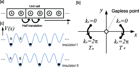
Figure 1: (a) Two inequivalent sites A and B in the unit cell. (b)Topologically different trajectories $(x(k_{x}),y(k_{x}))$. (c) Insulating state I (top) and II (bottom).

The Hamiltonian with the nonsymmorphic chiral symmetry has a generic form

$$H_{\rm 1D}(k_{x})=\begin{pmatrix}x(k_{x})&-iy(k_{x})e^{-ik_{x}/2}\\ iy(k_{x})e^{ik_{x}/2}&-x(k_{x})\end{pmatrix},$$ (4)

with real functions $x(k_{x})$ and $y(k_{x})$. The $2\pi$-periodicity of the Hamiltonian, $H_{\mathrm{1D}}(k_{x}+2\pi)=H_{\mathrm{1D}}(k_{x})$, implies

$$x(k_{x}+2\pi)=x(k_{x}),\quad y(k_{x}+2\pi)=-y(k_{x}).$$ (5)

Because the eigenvalues of the Hamiltonian are $E(k_{x})=\pm\sqrt{[x(k_{x})]^{2}+[y(k_{x})]^{2}},$ the system is gapped at $E=0$ unless the vector $(x(k_{x}),y(k_{x}))$ passes through the origin $(0,0)$ at some $k_{x}$.

Now we will show that the Hamiltonian (4) has two distinct topological phases: As we show in Fig.1(b), the Hamiltonian defines a trajectory of $(x(k_{x}),y(k_{x}))$ in the $xy$-plane, when $k_{x}$ changes from $0$ to $2\pi$. From the constraint of Eq.(5), the trajectory forms an open arc, not a closed circle, and the end point $(x(2\pi),y(2\pi))$ must be the mirror image of the start point $(x(0),y(0))$ with respect to the $x$-axis. The open trajectory passes the $x$-axis odd number of times. More precisely, we have two different ways to across the $x$-axis; if the trajectory pass the positive $x$-axis odd (even) number of times, then it must pass the negative $x$-axis even (odd) number of times. See trajectories ${\rm T}_{\rm o}$ and ${\rm T}_{\rm e}$ in Fig.1(c). These two different trajectories cannot be continuously deformed into each other without gap-closing, since they cannot across the origin without gap-closing, as mentioned in the above. Therefore, by counting the parity of times the trajectory passes the positive $x$-axis, we can identify the two distinct phases of the Hamiltonian (4). The $\bm{Z}_{2}$ nature of the topological phase is discussed in details in Ref.SM .

If the parity is odd (even), then the Hamiltonian is adiabatically deformed into the $k_{x}$-independent Hamiltonian $H_{\rm o}$ ($H_{\rm e}$) in the below, without gap-closing,

$$H_{\rm o}=-\sigma_{z},\quad H_{\rm e}=\sigma_{z},$$ (6)

with the Pauli matrix $\sigma_{i}$ $(i=0,x,y,z)$. These Hamiltonians suggest a simple physical realization of the nonsymmorphic chiral symmetry. Consider a periodic potential with two different local minima A and B in the unit cell. See Fig.1(c). If the energy of the local minimum A (B) is much higher than B’s (A’s) and tunnelings between local minima are neglected, we have an insulating phase I (II) in the half filling, which effective Hamiltonian is given by $H_{e}$ ($H_{o}$). Our argument above implies that these insulating phases are topologically distinct and they are separated by a topological quantum phase transition as long as one keeps the symmetry (2). Such a periodic system could be artificially created by cold atoms.

Nonsymmorphic $Z_{2}$ symmetry in 2D— Much more interesting $\bm{Z}_{2}$ topological phases protected by nonsymmorphic symmetries appear in two and three dimensions. In these dimensions, a class of nonsymmorphic symmetries are consistent with the presence of a surface, and thus the symmetry protected gapless edge states may appear. Here we present a 2D $\bm{Z}_{2}$-topological nonsymmorphic insulator, which supports a unique edge state.

To obtain the $\bm{Z}_{2}$ phase, we use a Hamiltonian map that increases the dimension of the system. This map keeps the topological structure by shifting symmetries, and is known to be useful to classify the topological (or topological crystalline) insulators/superconductorsTeo and Kane (2010); Shiozaki and Sato (2014). In particular, the periodic structure of the topological table is explained by this map. The details of the map in the present case and the relevant structure in the K-theory are given in Ref.SM .

From the Hamiltonian mapping, we obtain a representative Hamiltonian of a 2D $\bm{Z}_{2}$ topological nonsymmorphic insulator,

$$H_{\rm 2D}(k_{x},k_{y})=(m+\cos k_{y})\tau_{y}\otimes H_{\rm 1D}(k_{x})+\sin k_{y}\tau_{x}\otimes\sigma_{0},$$ (7)

which has a $k_{x}$-dependent nonsymmorphic symmetry

$$\left[U(k_{x}),H_{\rm 2D}(k_{x},k_{y})\right]=0,\quad U(k_{x})=\tau_{x}\otimes\Gamma_{\rm 1D}(k_{x}),$$ (8)

and the additional chiral symmetry,

$$\{\Gamma,H_{\rm 2D}(k_{x},k_{y})\}=0,\quad\Gamma=\tau_{z}\otimes\sigma_{0}$$ (9)

where $\tau_{i}$ ($i=0,1,2,3$) is the Pauli matrix for the degrees of freedom on which $\Gamma$ acts. These two symmetry operators anticommute

$$\{\Gamma,U_{\rm 2D}(k_{x})\}=0.$$ (10)

Here note that the nonsymmorphic symmetry $U_{\mathrm{2D}}(k_{x})$ commutes with $H_{\mathrm{2D}}(k_{x},k_{y})$, although it is constructed from $\Gamma_{\mathrm{1D}}(k_{x})$ anticommuting with $H_{\mathrm{1D}}(k_{x})$. Whereas any terms consistent with the symmetries (8) and (9) can be added to the Hamiltonian, the basic topological properties can be captured by Eq.(7). For a gapped $H_{\mathrm{1D}}(k_{x})$, the system has a gap unless $m=\pm 1$. Using the symmetries (8) and (9), we can define a $\bm{Z}_{2}$ invariant, which is nontrivial (trivial) if $-1<m<1$ ($m>1$ or $m<-1$)SM . Without loss of generality, we assume in the following that the parity of $H_{\mathrm{1D}}(k_{x})$ is even, so it is topologically equivalent to $H_{\mathrm{e}}=\sigma_{z}$.

If we consider a boundary parallel to the $x$-axis, we can keep the symmetries (8) and (9). This boundary supports gapless edge states when the system is topological ($-1<m<1$): To demonstrate this, consider a semi-infinite system $(y>0)$ with the edge at $y=0$. Since $H_{\mathrm{1D}}(k_{x})$ is topologically equivalent to $\sigma_{z}$, we first consider the spacial case of the Hamiltonian (7) with $H_{\mathrm{1D}}(k_{x})=\sigma_{z}$. In this particular case, the Hamiltonian $H_{\mathrm{2D}}(k_{x},k_{y})$ does not depend on $k_{x}$, and thus the topological edge state should be a $k_{x}$-independent zero energy state. The edge state can be obtained analytically when the system is close to the topological phase transition at $m=\pm 1$. Near the topological phase transition, say at $m=-1$, the bulk gap is nearly closed at $k_{y}=0$, so the low energy physics is well-described by the effective Hamiltonian obtained by the expansion of Eq.(7) around $k_{y}=0$. Then, replacing $k_{y}$ with $-i\partial_{y}$, we have the equation for the edge state

$$\left[(m+1+\partial_{y}^{2}/2)\tau_{y}\otimes\sigma_{z}-i\partial_{y}\tau_{x}\otimes\sigma_{0}\right]\psi(y)=0,$$ (11)

with the boundary condition $\psi(0)=0$ and $\psi(\infty)=0$. If the system is in the topological side near the transition i.e. $\delta m\equiv m+1>0$, the equation has two independent solutions localized at $y=0$

$$|\psi_{1}\rangle=\begin{pmatrix}1\\ 0\end{pmatrix}_{\tau}\otimes\begin{pmatrix}0\\ 1\end{pmatrix}_{\sigma}e^{-y}\sinh\left(\sqrt{-2\delta m+1}y\right)$$

$$|\psi_{2}\rangle=\begin{pmatrix}0\\ 1\end{pmatrix}_{\tau}\otimes\begin{pmatrix}1\\ 0\end{pmatrix}_{\sigma}e^{-y}\sinh\left(\sqrt{-2\delta m+1}y\right).$$ (12)

On the other hand, in the non-topological side ($\delta m<0$), the solutions are diverge, and the edge states disappear. A similar result is found near another transition point at $m=1$. We have also confirmed numerically the existence of the zero energy edge mode for the whole region of $-1<m<1$.

For a general $k_{x}$-dependent $H_{\mathrm{1D}}(k_{x})$, the zero energy edge states have a $k_{x}$-dependent energy dispersion. By diagonalizing the mixing matrix $\langle\psi_{i}|(\delta m+\partial_{y}^{2}/2)\tau_{y}\otimes(H_{\mathrm{1D}}(k_{x})-\sigma_{z})|\psi_{j}\rangle$, the energy is evaluated as $E(k_{y})\propto\pm y(k_{x})$. Then, from the constraint (5), there must be an odd number of zeros for $y(k_{x})$ in $k_{x}\in[0,2\pi]$, and thus the energy dispersion becomes helical $E(k_{y})\sim\pm c(k_{x}-k_{0})$ around each zero $k_{0}$, as illustrated in Fig.2 (a).

Since the Hamiltonian $H_{\mathrm{2D}}(k_{x},k_{y})$ commutes with $U(k_{x})$, the helical dispersion is decomposed into chiral and anti-chiral ones, each of which is an eigenstate of $U(k_{x})$. These two chiral dispersions are mapped to each other by the chiral symmetry $\Gamma$, because $\Gamma$ maps a gapless state to another one, reversing the slope of the dispersion. Furthermore, they belong to different eigensectors of $U(k_{x})$, because $\Gamma$ exchanges the eigenvalues of $U(k_{x})$ due to $\{\Gamma,U(k_{x})\}=0$. Therefore, these two chiral dispersions stay gapless without mixing, as far as the symmetries (8) and (9) are retained.

Whereas the above edge state has a similarity to helical edge modes in quantum spin Hall states, their overall structure in the momentum space is completely different: As is seen in Fig.2 (a), the present edge state has a unique energy dispersion with the Möbius twist, which is never seen in other ${\bm{Z}}_{2}$ phases. This twist occurs due to the multivalueness of the eigenvalues $u=\pm e^{-ik_{x}/2}$ of $U(k_{x})$: When one goes round in the $k_{x}$-direction as $k_{x}\rightarrow k_{x}+2\pi$, $u$ changes the sign, so a chiral dispersion in an eigensector of $U(k_{x})$ turns smoothly into to an anti-chiral one in another eigensector.

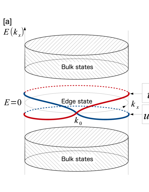
Figure 2: (color online). Schematic illustration of edge states with Möbius twist. (a) The red (blue) line is an edge state in the eigensector of $U(k_{x})$ with the eigenvalue $u=e^{-ik_{x}/2}$ ($u=-e^{-ik_{x}/2}$). (b) An exchange process of the eigensectors.

Another remarkable feature of our edge state is that the constituent chiral dispersions can exchange their eigensectors of $U(k_{x})$, as illustrated in Fig.2 (b). This means that any pair of helical dispersions is topologically unstable: When a pair of helical dispersions exits, we can always realize the situation where a chiral dispersion coexists with an anti-chiral one in the same eigensector of $U(k_{x})$, by exchanging the eigensectors properly. Thus, we can open a gap of helical dispersion by mixing between the chiral and anti-chiral ones.

The arguments above clearly indicate that helical edge states in this system has a $\bm{Z}_{2}$ stability like helical edge states in quantum spin Hall systems, although no time-reversal symmetry is required and the mechanism of the stability is completely different.

Glide reflection symmetry in 3D— Finally, we consider the system with glide reflection symmetry,

$$G(k_{x})H_{\rm 3D}(k_{x},k_{y},k_{z})G^{-1}(k_{x})=H_{\rm 3D}(k_{x},k_{y},-k_{z}),$$

$$G^{2}(k_{x})=e^{-ik_{x}},$$ (13)

The glide reflection $G(k_{x})$ is the combination of reflection with respect to the $xy$-plane and translation along the $x$-axis by a half of the lattice spacing. Since $G^{2}(k_{x})$ results in a translation by a unit lattice spacing in the $x$-direction, it provides the non-trivial $e^{-ik_{x}}$ factor. The $\bm{Z}_{2}$ invariant defined by the glide reflection symmetry is given in Ref.SM .

A representative Hamiltonian with glide reflection symmetry is given by SM

$$H_{\rm 3D}({\bm{k}}) = (m+\cos k_{z}+\cos k_{y})\tau_{y}\otimes H_{\rm 1D}(k_{x})$$

$$+ \sin k_{y}\tau_{x}\otimes\sigma_{0}+\sin k_{z}\tau_{z}\otimes\sigma_{0},$$

$$G(k_{x}) = \tau_{x}\otimes\Gamma_{\rm 1D}(k_{x}).$$ (14)

The 3D system is gapped unless $m=\pm 2,0$. The $\bm{Z}_{2}$ invariant is non-trivial (trivial) when $-2<m<0$ or $0<m<2$ ($m<-2$ or $m>2$) SM .

A surface perpendicular to the $y$-axis retains the glide reflection symmetry, so it may support a gapless surface state protected by this symmetry. For instance, consider a semi-infinite 3D system $(y>0)$ with a surface at $y=0$, which preserves the glide reflection symmetry. In a manner similar to the 2D system, for the special but topologically equivalent case with $H_{\mathrm{1D}}(k_{x})=\sigma_{z}$, we can obtain the surface state analytically near the topological phase transition at $m=\pm 2$: For $m\sim-2$, $H_{\mathrm{3D}}(\bm{k})$ is well approximated by

$$\hat{H}_{\mathrm{3D}} = (m+\cos k_{z}+1-\partial_{y}^{2}/2)\tau_{y}\otimes\sigma_{z}$$ (15)

$$- i\partial_{y}\tau_{x}\otimes\sigma_{0}+\sin k_{z}\tau_{z}\otimes\sigma_{0}.$$

We find that $|\psi_{1}\rangle$ and $|\psi_{2}\rangle$ in Eq.(12) with $\delta m=m+\cos k_{z}+1$ satisfy the Schrödinger equation,

$$\hat{H}_{\rm 3D}\psi_{i}(y)=E_{i}(k_{z})\psi_{i}(y),$$ (16)

with $E_{1}(k_{z})=\sin k_{z}$ and $E_{2}(k_{z})=-\sin k_{z}$, respectively. When the system is in the topological side near the transition, i.e. $-2<m<0$, $\delta m$ is positive (negative) at $k_{z}=0$ ($k_{z}=\pi$). Thus, they meet the boundary condition $\psi_{i}(0)=0$ and $\psi_{i}(\infty)=0$ near $k_{z}=0$, while they diverge near $k_{z}=\pi$. This means that they form surface states with the linear dispersion $E(k_{z})=\pm k_{z}$ near $k_{z}=0$, which merge into bulk states near $k_{z}=\pi$. On the other hand, in the topologically trivial side, i.e. $m<-2$, $\delta m$ is always negative, so $|\psi_{1}\rangle$ and $|\psi_{2}\rangle$ are no longer physical states anymore. A similar analysis works for $0<m<2$, although the surface states appear near $k_{z}=\pi$ in this case.

For a general $H_{\mathrm{1D}}(k_{x})$, the surface states have a dispersion in the $k_{x}$-direction, as well as in the $k_{z}$-direction: Like the 2D case, the two surface modes, $|\psi_{1}\rangle$ and $|\psi_{2}\rangle$, are mixed. The spectrum of the surface states becomes $E(k_{x},k_{z})=\pm\sqrt{cy^{2}(k_{x})+\sin^{2}k_{z}}$. ($c$ is a constant.) From the constraint (5), $y(k_{x})$ has an odd number of zeros, and thus the surface states have the corresponding odd number of Dirac cones in the spectrum, as illustrated in Fig.3.

In the glide invariant plane at $k_{z}=\Lambda$ ($\Lambda=0,\pi$) in the Brillouin zone, the Dirac cone has helical dispersions $E\sim\pm c(k_{x}-k_{0})$ in the $k_{x}$-direction. Since $H_{\rm 3D}({\bm{k}})$ commutes with $G(k_{x})$ at $k_{z}=\Lambda$, the helical dispersion can be divided into two eigensectors of $G(k_{x})$, which have chiral dispersion and anti-chiral dispersion, respectively. These two chiral dispersions cannot mix, so a single Dirac cone is topologically stable. On the other hand, a pair of Dirac cone is topologically unstable: From a process similar to Fig.2 (b), the eigensectors can exchange without gap-closing. Therefore, from a similar argument in the 2D case, helical dispersions for a pair of Dirac cones can be gapped.

As in the 2D case, the obtained surface state has a very unique feature: In the $k_{x}$-direction, which is the direction of the translation for the glide, the surface state has an energy dispersion with the Möbius twist. Furthermore, along the same direction, the surface state is detached from the bulk spectrum. Indeed, by adiabatically changing $H_{\mathrm{1D}}(k_{x})$ as $H_{\mathrm{1D}}=\sigma_{z}$, the surface state becomes completely flat at $E=0$ in the $k_{x}$-direction. This feature is never seen in surface Dirac modes in other ${\bm{Z}}_{2}$ phases. Any stable Dirac mode in other ${\bm{Z}}_{2}$ phases bridge the bulk conduction and valence bands in any direction in the surface Brillouin zone. This remarkable feature in the spectrum can be detected by angle-resolved photoemission, which provides a distinct evidence of this novel $\bm{Z}_{2}$ phase.

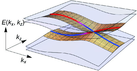
Figure 3: (color online). A surface state protected by glide reflection symmetry. The spectrum at $k_{z}=\Lambda$ has a Möbius twist in the $k_{x}$-direction: Along the $k_{x}$-direction, the red branch with the eigenvalue $e^{ik_{x}/2}$ of $G(k_{x})$ turns into the blue one with the eigenvalue $-e^{ik_{x}/2}$.

Summary— We have revealed that nonsymmorphic crystalline symmetries such as glide reflection symmetry provide a class of novel ${\bm{Z}}_{2}$ phases. They are related to each other by Hamiltonian mapping, which is justified by the K-theory SM . These ${\bm{Z}}_{2}$ phases predict remarkable surface states that have the Möbius twist in the spectrum, which can be detectable experimentally.

Note added— After this work was finalized, there appeared a complementary and independent work Fang and Fu which has some overlap with our results.

M.S is supported by the JSPS (No.25287085) and KAKENHI Grants-in-Aid (No.22103005) from MEXT. K.S. is supported by a JSPS Fellowship for Young Scientists, and K.G. is supported by the Grant-in-Aid for Young Scientists (B 23740051), JSPS.

Supplementary Material

Appendix A Hamiltonian mapping

Here we introduce a Hamiltonian mapping which relates topological phase in different dimensions. A similar map has been used in the classification of topological insulators and superconductors defined on a sphere ${\bm{k}}\in S^{d}$ in the momentum spaceTeo and Kane (2010); Shiozaki and Sato (2014). We generalize the idea to insulators with nonsymmorphic symmetries.

First we review the Hamiltonian mapping used in topological insulators and superconductors. The map is given as follows: If a Hamiltonian $H({\bm{k}})$ on a $d$-dimensional sphere ${\bm{k}}\in S^{d}$ has chiral symmetry, $\{\Gamma,H({\bm{k}})\}=0,$ with the chiral operator $\Gamma$, then the map is

$$H({\bm{k}},\theta)=\sin\theta H({\bm{k}})+\cos\theta\Gamma,\quad\theta\in[0,\pi],$$ (S1)

and if not, it is

$$H({\bm{k}},\theta)=\sin\theta\tau_{y}\otimes H({\bm{k}})+\cos\theta\tau_{x}\otimes{\bm{1}},\,\,\theta\in[0,\pi],$$ (S2)

where ${\bm{1}}$ is the unit matrix with the same dimension as $H({\bm{k}})$. Since the mapped Hamiltonian $H({\bm{k}},\theta)$ is independent of ${\bm{k}}\in S^{d}$ at $\theta=0$ and $\pi$, the base space $({\bm{k}},\theta)\in S^{d}\times[0,\pi]$ of $H({\bm{k}},\theta)$ can be regarded as a $(d+1)$-dimensional sphere $S^{d+1}$ by shrinking $S^{d}$ to a point at $\theta=0$ and $\pi$, respectively. Thus the mapped Hamiltonian $H({\bm{k}},\theta)$ is defined on $S^{d+1}$. Furthermore, it can be shown that the map is isomorphic and thus the original $H({\bm{k}})$ and the mapped $H({\bm{k}},\theta)$ have the same topological structures. This map relates topological insulators in different dimensions, and it enables us to study their topological phases systematically.

Using the above isomorphic map, we can construct the 2D insulator

$$H_{\rm 2D}(k_{x},k_{y})=(m+\cos k_{y})\tau_{y}\otimes H_{\rm 1D}(k_{x})$$

$$+\sin k_{y}\tau_{x}\otimes\sigma_{0},$$ (S3)

with symmetries

$$\left[U(k_{x}),H_{\rm 2D}(k_{x},k_{y})\right]=0,\quad U(k_{x})=\tau_{x}\otimes\Gamma_{\rm 1D}(k_{x}),$$

$$\{\Gamma,H_{\rm 2D}(k_{x},k_{y})\}=0,\quad\Gamma=\tau_{z}\otimes\sigma_{0},$$ (S4)

which is topologically nontrivial (trivial) for $-1<m<1$ ($m>1$ or $m<-1$).

The basic idea is as follows: For $H_{\rm 1D}({\bm{k}})$ on $k_{x}\in S^{1}$, consider the following two Hamiltonians defined on $(k_{x},\theta)\in S^{1}\times[0,\pi]$,

$$H_{\rm R}(k_{x},\theta)=\sin\theta\tau_{y}\otimes H_{\rm 1D}(k_{x})+\cos\theta\tau_{x}\otimes\sigma_{0},$$

$$H_{\rm L}(k_{x},\theta)=\sin\theta\tau_{y}\otimes[-H_{\rm 1D}(k_{x})]+\cos\theta\tau_{x}\otimes\sigma_{0},$$ (S5)

which are obtained by the isomorphic map (S2). They have the symmetry,

$$[U(k_{x}),H_{{\rm R},{\rm L}}(k_{x},\theta)]=0,\quad\{\Gamma,H_{{\rm R},{\rm L}}(k_{x},\theta)\}=0,$$ (S6)

with $U(k_{x})=\tau_{x}\otimes\Gamma_{\rm 1D}(k_{x})$ and $\Gamma=\tau_{z}\otimes\sigma_{0}$. Since $H_{\rm 1D}(k_{x})$ and $-H_{\rm 1D}(k_{x})$ have different ${\bm{Z}}_{2}$ numbers, either $H_{\rm R}(k_{x},\theta)$ or $H_{\rm L}(k_{x},\theta)$, but not both is topologically nontrivial. These two Hamiltonians coincide at $\theta=0$ and $\pi$, respectively. Thus, by sewing these two Hamiltonians at $\theta=0$ and $\pi$, as illustrated in Fig.4, we can obtain a system defined on a two-dimensional torus $T^{2}$. The resultant system has a non-trivial $\bm{Z}_{2}$ number, which is obtained as the total $\bm{Z}_{2}$ numbers of $H_{\rm R}(k_{x},\theta)$ and $H_{\rm L}(k_{x},\theta)$.

To obtain an explicit Hamiltonian of the system on $T^{2}$, we change the variable $\theta$ as $\theta=\pi/2-k_{y}$ in $H_{\rm R}(k_{x},\theta)$ and $\theta=k_{y}-\pi/2$ in $H_{\rm L}(k_{x},\theta)$, respectively. For the new variable, $H_{\rm R}$ and $H_{\rm L}$ have the same form as $H_{\rm 2D}(k_{x},k_{y})$

$$H_{\rm 2D}(k_{x},k_{y})=\cos k_{y}\tau_{y}\otimes H_{\rm 1D}(k_{x})+\sin k_{y}\tau_{x}\otimes\tau_{0},$$ (S7)

where $H_{\rm L}$ and $H_{\rm R}$ are smoothly connected at $k_{y}=\pi/2$ and $k_{y}=-\pi/2$, respectively. Equation (S7) is the Hamiltonian of the sewn system. Note that we may adiabatically add a term preserving the symmetries (S6) to the Hamiltonian without changing its topological property unless the bulk gap of the system closes. Thus we can finally modify (S7) in the form of Eq.(S3) with $-1<m<1$.

In a similar manner, we can obtain a system on $T^{2}$ with trivial ${\bm{Z}}_{2}$ topology. In this case, we use the same Hamiltonian for $H_{\rm R}(k_{x},\theta)$ and $H_{\rm L}(k_{x},\theta)$,

$$H_{\rm R}(k_{x},\theta)=H_{\rm L}(k_{x},\theta)$$

$$=\sin\theta\tau_{y}\otimes H_{\rm 1D}(k_{x})+\cos\theta\tau_{x}\otimes\sigma_{0},$$ (S8)

with $\theta\in[0,\pi]$. Even when $H_{\rm R}$ and $H_{\rm L}$ have non-trivial $\bm{Z}_{2}$ numbers, they are canceled by sewing them at $\theta=0$ and $\theta=\pi$. An explicit form of the sewn Hamiltonian is obtained as follows. Because $\sin\theta\geq 0$, we can add a positive constant $m$ to $\sin\theta$ in Eq.(S8) without gap-closing,

$$H_{\rm R}(k_{x},\theta)=H_{\rm L}(k_{x},\theta)$$

$$=(m+\sin\theta)\tau_{y}\otimes H_{\rm 1D}(k_{x})+\cos\theta\tau_{x}\otimes\sigma_{0},$$ (S9)

where we gradually increase $m$ as it satisfies $m>1$. Then we can adiabatically change the coefficient of $\sin\theta$ in $H_{\rm L}(k_{x},\theta)$ as $\sin\theta\rightarrow-\sin\theta$, without gap-closing. As a result, $H_{\rm R}$ and $H_{\rm L}$ can be

$$H_{\rm R}(k_{x},\theta)=(m+\sin\theta)\tau_{y}\otimes H_{\rm 1D}(k_{x})+\cos\theta\tau_{x}\otimes\sigma_{0},$$

$$H_{\rm L}(k_{x},\theta)=(m-\sin\theta)\tau_{y}\otimes H_{\rm 1D}(k_{x})+\cos\theta\tau_{x}\otimes\sigma_{0},$$ (S10)

with $m>1$. Finally, by changing the variable $\theta$ as $\theta=\pi/2-k_{y}$ in $H_{\rm R}(k_{x},\theta)$ and $\theta=k_{y}-\pi/2$ in $H_{\rm L}(k_{x},\theta)$, respectively, we find that $H_{\rm R}$ and $H_{\rm L}$ have the form of Eq.(S3) with $m>1$, where $H_{\rm R}$ and $H_{\rm L}$ are smoothly sewn up at $k_{y}=\pm\pi/2$. We note that if we take the starting Hamiltonians as

$$H_{\rm R}(k_{x},\theta)=H_{\rm L}(k_{x},\theta)$$

$$=\sin\theta\tau_{y}\otimes[-H_{\rm 1D}(k_{x})]+\cos\theta\tau_{x}\otimes\sigma_{0},$$ (S11)

we can obtain Eq.(S3) with $m<-1$, in a similar manner.

The same idea is available to obtain the 3D insulators

$$H_{\rm 3D}({\bm{k}}) = (m+\cos k_{z}+\cos k_{y})\tau_{y}\otimes H_{\rm 1D}(k_{x})$$ (S12)

$$+ \sin k_{y}\tau_{x}\otimes\tau_{0}+\sin k_{z}\tau_{z}\otimes\tau_{0},$$

with the glide reflection symmetry,

$$G(k_{x})H_{\rm 3D}(k_{x},k_{y},k_{z})G^{-1}(k_{x})=H_{\rm 3D}(k_{x},k_{y},-k_{z}),$$

$$G(k_{x})=\tau_{x}\otimes\Gamma_{\rm 1D}(k_{x}),$$ (S13)

which is $\bm{Z}_{2}$-non-trivial ($\bm{Z}_{2}$-trivial) for $-2<m<0$ or $0<m<2$ ($m<-2$ or $m>2$): Since $H_{\rm 2D}$ in Eq.(S3) is chiral symmetric, we use the isomorphic map (S1) to have $H_{\rm R}(k_{x},k_{y},\theta)$ and $H_{\rm L}(k_{x},k_{y},\theta)$,

$$H_{\rm R}(k_{x},k_{y},\theta)=\sin\theta H_{\rm 2D}(k_{x},k_{y})+\cos\theta\Gamma,$$

$$H_{\rm L}(k_{x},k_{y},\theta)=\sin\theta H^{\prime}_{\rm 2D}(k_{x},k_{y})+\cos\theta\Gamma,$$ (S14)

where we denote $H_{\rm 2D}$ in $H_{\rm L}$ as $H_{\rm 2D}^{\prime}$ as it can be different from $H_{\rm 2D}$ in $H_{\rm R}$. $H_{\rm R}$ and $H_{\rm L}$ have the same $\bm{Z}_{2}$ topological number as $H_{\rm 2D}$ and $H_{\rm 2D}^{\prime}$, respectively. By jointing $H_{\rm R}$ and $H_{\rm L}$ at $\theta=0$ and $\pi$, we can have a Hamiltonian $H_{\rm 3D}$ defined on a 3D torus $T^{3}$. If either $H_{\rm R}$ or $H_{\rm L}$, but not both is ${\bm{Z}}_{2}$-nontrivial, $H_{\rm 3D}$ is $\bm{Z}_{2}$-nontrivial. In other cases, $H_{\rm 3D}$ is $\bm{Z}_{2}$-trivial. Then, one can show that with a suitable adiabatic deformation, $H_{\rm 3D}$ takes the form of Eq.(S12) without gap-closing.

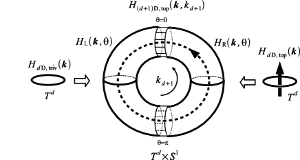
Figure 4: Hamiltonian mapping. Two Hamiltonians $H_{\rm R}({\bm{k}},\theta)$ and $H_{\rm R}({\bm{k}},\theta)$ defined on $T^{d}\times[0,\pi]$ are sewn at $\theta=0$ and $\pi$.

Appendix B $\bm{Z}_{2}$ invariants for nonsymmorphic systems

B.1 1D case

Here we generalize the $\bm{Z}_{2}$ invariant defined for the simplest $2\times 2$ Hamiltonian (4) in the main text, to that for the general Hamiltonian.

The nonsymmorphic chiral symmetry is given by

$$\{\Gamma_{1D}(k_{x}),H_{\rm 1D}(k_{x})\}=0,\quad\Gamma^{2}_{\rm 1D}(k_{x})=e^{-ik_{x}}.$$ (S15)

By imposing $2\pi$-periodicity in $k_{x}$ on $\Gamma_{\rm 1D}(k_{x})$, a general form of $\Gamma_{\rm 1D}(k_{x})$ is given by

$$\Gamma_{\rm 1D}(k_{x})=\begin{pmatrix}0&e^{-ik_{x}}\\ 1&0\end{pmatrix}\otimes{\bm{1}}_{N\times N},$$ (S16)

with the $N\times N$ unit matrix ${\bm{1}}_{N\times N}$. In this basis, the Hamiltonian $H_{\rm 1D}(k_{x})$ with the nonsymmorphic chiral symmetry takes the form

$$H_{\rm 1D}(k_{x})=\begin{pmatrix}X(k_{x})&-iY(k_{x})e^{-ik_{x}/2}\\ iY(k_{x})e^{ik_{x}/2}&-X(k_{x})\end{pmatrix},$$ (S17)

where $X(k_{x})$ and $Y(k_{x})$ are $N\times N$ hermitian matrices. Since $H_{\rm 1D}(k_{x})$ is $2\pi$-periodic in $k_{x}$, $X(k_{x})$ and $Y(k_{x})$ satisfy

$$X(k_{x}+2\pi)=X(k_{x}),\quad Y(k_{x}+2\pi)=-Y(k_{x}).$$ (S18)

Now we introduce the following $N\times N$ matrix $Z(k_{x})$

$$Z(k_{x})=X(k_{x})+iY(k_{x}),$$ (S19)

which has the constraint

$$Z(k_{x}+2\pi)=Z^{\dagger}(k_{x}).$$ (S20)

Because one can prove the relation

$${\rm det}H_{\rm 1D}(k_{x})=|{\rm det}Z(k_{x})|^{2},$$ (S21)

${\rm det}Z(k_{x})\neq 0$ when $H_{\rm 1D}(k_{x})$ is gapped at $E=0$ (namely, when ${\rm det}H_{\rm 1D}(k_{x})\neq 0$).

Denoting the real and imaginary parts of ${\rm det}Z(k_{x})$ as $x(k_{x})$ and $y(k_{x})$, respectively, the relation (S21) implies $x^{2}(k_{x})+y^{2}(k_{x})\neq 0$ for a gapped $H_{\rm 1D}(k_{x})$. Furthermore, from Eq.(S20), we have

$$x(k_{x}+2\pi)=x(k_{x}),\quad y(k_{x}+2\pi)=-y(k_{x}).$$ (S22)

Since $x(k_{x})$ and $y(k_{x})$ defined here have the same property as those in the main text, we can define the $\bm{Z}_{2}$ invariant in the same manner.

As is shown in the main text, the simplest Hamiltonian with the non-trivial ${\bm{Z}}_{2}$ invariant is $H_{\rm o}=-\sigma_{z}$, which gives $(x(k_{x}),y(k_{x}))=(-1,0)$. To confirm the ${\bm{Z}}_{2}$ nature, consider the direct sum $H_{\rm o}\oplus H_{\rm o}$. In the basis where $\Gamma_{\rm 1D}(k_{x})$ takes the form of Eq.(S16), $H_{\rm o}\oplus H_{\rm o}$ gives $X(k_{x})=-{\bm{1}}_{2\times 2}$ and $Y(k_{x})=0$. Thus, we find $(x(k_{x}),y(k_{x}))=(1,0)$ for $H_{\rm o}\oplus H_{\rm o}$, which implies that $H_{\rm o}\oplus H_{\rm o}$ is ${\bm{Z}}_{2}$-trivial.

B.2 2D case

In this section, we define the $\bm{Z}_{2}$ invariant for the 2D Hamiltonian which has the nonsymmorphic symmetry

$$\left[U(k_{x}),H_{\rm 2D}(k_{x},k_{y})\right]=0,\quad U(k_{x})^{2}=e^{-ik_{x}},$$ (S23)

as well as the ordinary chiral symmetry,

$$\{H_{\rm 2D}(k_{x},k_{y}),\Gamma\}=0,\quad\Gamma^{2}=1.$$ (S24)

These symmetries are anticommute,

$$\{\Gamma,U(k_{x})\}=0.$$ (S25)

Consider the Schrödinger equation given by

$$H_{\rm 2D}(k_{x},k_{y})|u_{n}(k_{x},k_{y})\rangle=E_{n}(k_{x},k_{y})|u_{n}(k_{x},k_{y})\rangle,$$ (S26)

where $n$ is the band index. We assume that the system is gapped at $E=0$, and the Fermi energy is inside the gap. It is convenient here to use a positive (negative) $n$ to represent a positive (negative) energy band.

Since $H_{\rm 2D}(k_{x},k_{y})$ commutes with $U(k_{x})$, the solution $|u_{n}(k_{x},k_{y})\rangle$ are taken as eigenstates of $U(k_{x})$

$$U(k_{x})|u_{n}^{\pm}(k_{x},k_{y})\rangle=\pm e^{-ik_{x}/2}|u_{n}^{\pm}(k_{x},k_{y})\rangle.$$ (S27)

The chiral symmetry implies that if $|u_{n}^{\pm}(k_{x},k_{y})\rangle$ is a positive (negative) energy band, $\Gamma|u_{n}^{\pm}(k_{x},k_{y})\rangle$ is a negative (positive) energy band. From the anticommutation relation (S25), it is also found that $\Gamma|u_{n}^{\pm}(k_{x},k_{y})\rangle$ is an eigenstate of $U(k_{x})$ with the eigenvalue $\mp e^{ik_{x}/2}$. Therefore, we can place the relation

$$|u_{n}^{\pm}(k_{x},k_{y})\rangle=\Gamma|u_{-n}^{\mp}(k_{x},k_{y})\rangle.$$ (S28)

A key character of the nonsymmorphic symmetry $U(k_{x})$ is that its eigenvalues $\pm e^{-ik_{x}/2}$ do not have the same periodicity as $U(k_{x})$ itself: They change their sign when $k_{x}\rightarrow k_{x}+2\pi$. As a result, $|u_{n}^{+}(k_{x},k_{y})\rangle$ and $|u_{n}^{-}(k_{x}+2\pi,k_{y})\rangle$ have the same eigenvalue of $U(k_{x})$, satisfying the same Schrödinger equation. Thus, they are the same state up to a $U(1)$ gauge factor,

$$|u_{n}^{+}(k_{x}+2\pi,k_{y})\rangle=e^{i\theta_{n}(k_{x},k_{y})}|u_{n}^{-}(k_{x},k_{y})\rangle.$$ (S29)

This relation gives a non-trivial relation in Berry phases: Introducing the gauge field in the momentum space,

$$A_{i}^{\pm}(k_{x},k_{y})=i\sum_{n<0}\langle u_{n}^{\pm}(k_{x},k_{y})|\partial_{k_{i}}u_{n}^{\pm}(k_{x},k_{y})\rangle,$$ (S30)

we define the Berry phases $\gamma^{\pm}(k_{x})$ as

$$e^{i\gamma^{\pm}(k_{x})}=\exp\left(i\oint dk_{y}A_{y}^{\pm}(k_{x},k_{y})\right).$$ (S31)

Since Eq.(S29) implies

$$A_{i}^{\pm}(k_{x}+2\pi,k_{y})=A_{i}^{\mp}(k_{x},k_{y})-\sum_{n<0}\partial_{k_{i}}\theta_{n}(k_{x},k_{y}),$$ (S32)

the Berry phases satisfy

$$e^{i\gamma^{+}(k_{x}+2\pi)}=e^{i\gamma^{-}(k_{x})}e^{-i\oint dk_{y}\sum_{n<0}\partial_{k_{y}}\theta_{n}(k_{x},k_{y})}.$$ (S33)

From the periodicity in $k_{y}$, the integral $\oint dk_{y}\partial_{k_{y}}\theta_{n}$ should be $2\pi N_{n}$ with a integer $N_{n}$, and thus we have

$$e^{i\gamma^{+}(k_{x}+2\pi)}=e^{i\gamma^{-}(k_{x})}.$$ (S34)

Now we use Eq.(S28). This equation implies

$$A_{i}^{+}(k_{x},k_{y})+A_{i}^{-}(k_{x},k_{y})$$

$$=i\sum_{n}\langle u_{n}^{+}(k_{x},k_{y})|\partial_{k_{i}}u_{n}^{+}(k_{x},k_{y})\rangle,$$ (S35)

where the summation in the right hand side is taken for all $n$. Therefore, from the completeness relation, we find that $A_{i}^{+}(k_{x},k_{y})+A_{i}^{-}(k_{x},k_{y})$ is a total derivative of a function, which yields

$$e^{i[\gamma^{+}(k_{x})+i\gamma^{-}(k_{x})]}=1.$$ (S36)

Combining this with Eq.(S34), we finally have

$$e^{i\gamma^{+}(k_{x}+2\pi)}=e^{-i\gamma^{+}(k_{x})}.$$ (S37)

Using this relation, we can define the $\bm{Z}_{2}$ invariant in the same manner as the 1D case: Denoting the real and imaginary parts of $e^{i\gamma^{+}(k_{x})}$ as $x(k_{x})$ and $y(k_{x})$, respectively, we can introduce a nonzero two-dimensional vector $(x(k_{x}),y(k_{x}))$. Then Eq.(S37) gives the constraint

$$x(k_{x}+2\pi)=x(k_{x}),\quad y(k_{x}+2\pi)=-y(k_{x}),$$ (S38)

which is exactly the same as Eq.(5). Therefore, if the trajectories $(x(k_{x}),y(k_{x}))$ passes the positive $x$-axis odd (even) number of times, the system is topologically non-trivial (trivial).

The ${\bm{Z}}_{2}$ invariant of the Hamiltonian (7) is evaluated as follows. It is sufficient to consider the case with $H_{\rm 1D}(k_{x})=\sigma_{z}$ since $H_{\rm 1D}(k_{x})$ can deform into $\sigma_{z}$ without gap-closing. $H_{\rm 2D}(k_{x},k_{y})$ is block diagonal in the diagonal basis of $U(k_{x})$, and in the sector with the eigenvalue $u=\pm e^{-ik_{x}/2}$ of $U(k_{x})$, it is given by

$$H_{\rm 2D}^{\pm}=\pm\begin{pmatrix}\sin k_{y}&i(m+\cos k_{y})\\ -i(m+\cos k_{y})&-\sin k_{y}\end{pmatrix}.$$ (S39)

From this, we obtain

$$\gamma^{\pm}(k_{x})=\left\{\begin{array}[]{ll}0,&\mbox{for $m<-1$}\\ \pi,&\mbox{for $-1<m<1$}\\ 0,&\mbox{for $m>1$}\end{array}\right.,$$ (S43)

which implies the ${\bm{Z}}_{2}$ invariant is non-trivial (trivial) if $-1<m<1$ ($m>1$ or $m<-1$).

B.3 3D case

Finally, we define the $\bm{Z}_{2}$ topological invariant associated with glide symmetry

$$G(k_{x})H_{\rm 3D}(k_{x},k_{y},k_{z})G^{-1}(k_{x})=H_{\rm 3D}(k_{x},k_{y},-k_{z}),$$

$$G^{2}(k_{x})=e^{-ik_{x}}.$$ (S44)

From solutions of the Schrödinger equation

$$H_{\rm 3D}({\bm{k}})|u_{n}({\bm{k}})\rangle=E_{n}({\bm{k}})|u_{n}({\bm{k}})\rangle,$$ (S45)

we introduce the gauge field $A_{i}({\bm{k}})$ in the momentum space,

$$A_{i}({\bm{k}})=i\sum_{E_{n}({\bm{k}})<E_{\rm F}}\langle u_{n}({\bm{k}})|\partial_{k_{i}}u_{n}({\bm{k}})\rangle,$$ (S46)

where $E_{\rm F}$ is the Fermi energy. On the glide invariant plane at $k_{z}=\Lambda$ ($\Lambda=0,\pi$), the glide operator $G(k_{x})$ commutes with $H_{\rm 3D}$,

$$[G(k_{x}),H_{\rm 3D}(k_{x},k_{y},\Lambda)]=0,$$ (S47)

and thus the solutions of the Schrödinger equation are simultaneously eigenstates of $G(k_{x})$,

$$G(k_{x})|u_{n}^{\pm}(k_{x},k_{y},\Lambda)\rangle=\pm e^{-ik_{x}/2}|u_{n}^{\pm}(k_{x},k_{y},\Lambda)\rangle.$$ (S48)

Correspondingly, we can decompose $A_{i}({\bm{k}})$ into two parts,

$$A_{i}(k_{x},k_{y},\Gamma)=A_{i}^{+}(k_{x},k_{y},\Lambda)+A_{i}^{-}(k_{x},k_{y},\Lambda)$$ (S49)

with

$$A_{i}^{\pm}(k_{x},k_{y},\Lambda)$$

$$=i\sum_{E_{n}<E_{\rm F}}\langle u_{n}^{\pm}(k_{x},k_{y},\Lambda)|\partial_{k_{i}}u_{n}^{\pm}(k_{x},k_{y},\Lambda)\rangle.$$ (S50)

In a manner similar to $U(k_{x})$ in 2D, the eigenvalues of $G(k_{x})$ do not have the same periodicity in $k_{x}$ as $G(k_{x})$ itself, and they change their sign when $k_{x}\rightarrow k_{x}+2\pi$. As a result, we have a twisted boundary condition,

$$|u_{n}^{\pm}(k_{x}+2\pi,k_{y},\Lambda)\rangle=e^{i\theta^{\pm}_{n}(k_{x},k_{y},\Lambda)}|u_{n}^{\pm}(k_{x},k_{y},\Lambda)\rangle,$$ (S51)

where $\theta_{n}^{\pm}(k_{x},k_{y},\Lambda)$ is a $U(1)$ phase.

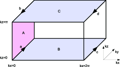
Figure 5: Upper half Brillouin zone.

Now we consider the upper half region of the Brillouin zone in Fig.5. From the twisted boundary condition, the Berry phases $\gamma^{\pm}(\ell)$ along $\ell=a,b,c,d$ in Fig.5,

$$\gamma^{\pm}(\ell)=\oint_{\ell}dk_{y}A_{y}^{\pm}(k_{x},k_{y},\Lambda)$$ (S52)

satisfy

$$\gamma^{+}(a)=\gamma^{-}(c)\,\,(\mbox{mod. 2$\pi$}),$$

$$\gamma^{+}(b)=\gamma^{-}(d)\,\,(\mbox{mod. 2$\pi$}).$$ (S53)

The Stokes’s theorem also leads to

$$\gamma(a+b)=\int_{A}F_{yz}dk_{y}dk_{z}\,\,(\mbox{mod. 2$\pi$}),$$

$$\gamma^{\pm}(c-a)=\int_{B}F^{\pm}_{xy}dk_{x}dk_{y}\,\,(\mbox{mod. 2$\pi$}),$$

$$\gamma^{\pm}(b-d)=\int_{C}F^{\pm}_{xy}dk_{x}dk_{y}\,\,(\mbox{mod. 2$\pi$}),$$ (S54)

with $\gamma(\ell)=\gamma^{+}(\ell)+\gamma^{-}(\ell)$, $F_{yz}=\partial_{k_{y}}A_{z}-\partial_{k_{y}}A_{z}$, and $F_{xy}^{\pm}=\partial_{k_{x}}A^{\pm}_{y}-\partial_{k_{y}}A^{\pm}_{x}$. The modular equality in the above equations comes from the ambiguity of the Berry phases.

Using these relations, we find that the following $\nu$ defines the $\bm{Z}_{2}$ invariant $(-1)^{\nu}$:

$$\nu = \frac{1}{2\pi}\left[\int_{A}F_{yz}dk_{y}dk_{z}+\int_{B-C}F^{-}_{xy}dk_{x}dk_{y}\right]$$ (S55)

$$- \frac{1}{\pi}\gamma^{+}(a+b)\,\,(\mbox{mod. 2}).$$

Here note that the modulo-2 ambiguity from the Berry phase $\gamma^{+}(a+b)$ does not affect on the $\bm{Z}_{2}$ invariant $(-1)^{\nu}$. In order for $(-1)^{\nu}$ to define the $\bm{Z}_{2}$ invariant, $\nu$ must be an integer. From Eqs.(S54) and (S53), we find that

$$\frac{1}{2\pi}\int_{B-C}F^{-}_{xy}dk_{x}dk_{y}$$

$$=\frac{1}{2\pi}\gamma^{-}(c-a-b+d)$$

$$=\frac{1}{2\pi}\left[\gamma^{-}(c+d)-\gamma^{-}(a+b)\right]$$

$$=\frac{1}{2\pi}\left[\gamma^{+}(a+b)-\gamma^{-}(a+b)\right]\,\,(\mbox{mod. 1}).$$ (S56)

Therefore, $\nu$ is recast into

$$\nu = \frac{1}{2\pi}\left[\int_{A}F_{yz}dk_{y}dk_{z}-\gamma(a+b)\right]\,\,(\mbox{mod. 1}),$$ (S57)

which takes an integer.

From the formula (S55), we can calculate the ${\bm{Z}}_{2}$ invariant $(-1)^{\nu}$ for $H_{\rm 3D}({\bm{k}})$ in Eq.(14). Since the ${\bm{Z}}_{2}$ invariant takes the same value unless the gap of the system closes, we can choose the special case of $H_{\rm 1D}(k_{x})=\sigma_{z}$. In this case, the first and the second terms of the right hand side of Eq.(S55) vanish, and thus we only need to evaluate $\gamma^{+}(a+b)$. On the glide invariant plane at $k_{z}=\Lambda$, $H_{\rm 3D}(k_{x},k_{y},\Lambda)$ is decomposed into $H_{\rm 3D}^{\pm}$ in the sector with the eigenvalue $\pm e^{-ik_{x}/2}$ of $G(k_{x})$,

$$H_{\rm 3D}^{\pm}(k_{x},k_{y},\Lambda)$$

$$=\pm\begin{pmatrix}\sin k_{y}&i(m+\cos\Lambda+\cos k_{y})\\ -i(m+\cos\Lambda+\cos k_{y})&-\sin k_{y}\end{pmatrix}.$$

From this, we find that

$$\gamma^{+}(a)=\left\{\begin{array}[]{ll}0,&\mbox{for $m<-2$}\\ \pi,&\mbox{for $-2<m<0$}\\ 0,&\mbox{for $m>0$}\end{array}\right.,$$ (S62)

$$\gamma^{+}(b)=\left\{\begin{array}[]{ll}0,&\mbox{for $m<0$}\\ \pi,&\mbox{for $0<m<2$}\\ 0,&\mbox{for $m>2$}\end{array}\right.,$$ (S66)

which implies

$$\nu=\left\{\begin{array}[]{ll}0,&\mbox{for $m<-2$}\\ 1,&\mbox{for $-2<m<0$}\\ 1,&\mbox{for $0<m<2$}\\ 0,&\mbox{for $m>2$}\end{array}\right.,$$ (S71)

modulo 2. Therefore, $H_{\rm 3D}({\bm{k}})$ in Eq.(14) is topologically non-trivial (trivial) if $-2<m<0$ or $0<m<2$ ($m>1$ or $m<-1$).

Appendix C K-theory analysis

We summarize relevant results in the $K$-theory. Consider a class of nonsymmorphic symmetries, $\{U|\tau_{x}\}$, which consist of a point group operation $U$ accompanying a half translation $\tau_{x}$ of the lattice spacing in the $x$-direction. We assume that the point group operation $U$ is a $\mathbb{Z}_{2}$-transformation (namely order-two). The nonsymmorphic symmetry $\{U|\tau_{x}\}$ acts on the Bloch Hamiltonian $H({\bm{k}})$ as a $k_{x}$-dependent unitary transformation $U(k_{x})$ with $U^{2}(k_{x})=e^{-ik_{x}/2}$.

Let us denote the K-group for $d$-dimensional insulators with the nonsymmorphic symmetry $U(k_{x})$ as $K_{\mathbb{Z}_{2}}^{(s,t,\tau_{x})}(T^{d})$. Here the superscript $(s,t,\tau_{x})$ identifies the symmetries of the insulators: $s=0,1$ (mod.$2$) indicates the absence ($s=0$) or the presence ($s=1$) of the additional chiral symmetry. Then $t=0,1$ (mod.$2$) determines how the point group operation of $U(k_{x})$ acts; for $s=0$, $t$ specifies the action of $U(k_{x})$ as Shiozaki and Sato (2014),

$$U(k_{x})H(k_{x},\bm{k})U(k_{x})^{-1}=\left\{\begin{array}[]{ll}H(k_{x},\tilde{\bm{k}})&(t=0),\\ -H(k_{x},\tilde{\bm{k}})&(t=1),\\ \end{array}\right.$$ (S74)

and for $s=1$,

$$\{H(k_{x},\bm{k}),\Gamma\}=0,\quad U(k_{x})H(k_{x},\bm{k})U(k_{x})^{-1}=H(k_{x},\tilde{\bm{k}}),$$

$$\Gamma U(k_{x})=\left\{\begin{array}[]{ll}U(k_{x})\Gamma&(t=0),\\ -U(k_{x})\Gamma&(t=1),\end{array}\right.,$$ (S77)

where $\bm{k}\mapsto\tilde{\bm{k}}$ represents a $\mathbb{Z}_{2}$ transformation for $T^{d-1}$. Finally, $\tau_{x}$ represents the half translation in the $x$-direction, as mentioned above. $(t,\tau_{x})$ is an example of a twisting of the twisted equivariant $K$-theory for topological insulators and superconductors. Freed and Moore (2013)

From the Gysin exact sequence Karoubi (2008) in the $K$-theory (the twisted version follows from the Thom isomorphism theorem Freed et al. (2011)), for $S^{1}$ except in the $k_{x}$-direction, the following isomorphism can be shown,

$$K_{\mathbb{Z}_{2}}^{(s,t,\tau_{x})}(T^{d}\times S^{1})$$

$$\cong K_{\mathbb{Z}_{2}}^{(s,t,\tau_{x})}(T^{d})\oplus K_{\mathbb{Z}_{2}}^{(s-1,t,\tau_{x})}(T^{d}),$$ (S78)

if $U(k_{x})$ for $K_{\mathbb{Z}_{2}}^{(s,t,\tau_{x})}(T^{d}\times S^{1})$ acts on $S^{1}$ as a global symmetry, or

$$K_{\mathbb{Z}_{2}}^{(s,t,\tau_{x})}(T^{d}\times S^{1})$$

$$\cong K_{\mathbb{Z}_{2}}^{(s,t,\tau_{x})}(T^{d})\oplus K_{\mathbb{Z}_{2}}^{(s-1,t-1,\tau_{x})}(T^{d}),$$ (S79)

if $U(k_{x})$ for $K_{\mathbb{Z}_{2}}^{(s,t,\tau_{x})}(T^{d}\times S^{1})$ acts on $S^{1}$ as a reflection symmetry. By iterating Eqs. (S78) and (S79), any K-group in the present case reduces to that for a $1$-dimensional nonsymmorphic insulator defined in the $k_{x}$-direction. The Hamiltonian mapping $d=1\to d=2\to d=3$ discussed previously is based on the isomorphism (S78) and (S79). In Eq. (S78) or (S79), the first term $K_{\mathbb{Z}_{2}}^{(n,t,\tau_{x})}(T^{d})$ in the right hand side represents a “weak” topological index of the left hand side, which is obtained by just neglecting the $S^{1}$-dependence in the left hand side, but the second term gives the “strong” topological index.

References

Kane and Mele (2005)
C. L. Kane and
E. J. Mele,
Phys. Rev. Lett. 95,
146802 (2005).
Bernevig and Zhang (2006)
B. A. Bernevig and
S. Zhang,
Phys. Rev. Lett. 96,
106802 (2006).
Moore and Balents (2007)
J. Moore and
L. Balents,
Phys. Rev. B 75,
121306 (2007).
Fu (2007)
L. Fu, Phys.
Rev. B 76, 045302
(2007).
Roy (2009)
R. Roy, Phys.
Rev. B 79, 195322
(2009).
Volovik (2003)
G. E. Volovik,
The universe in a helium droplet
(Clarendon Press, 2003), ISBN
0199564841.
Read and Green (2000)
N. Read and
D. Green,
Phys. Rev. B 61,
10267 (2000).
Kitaev (2001)
A. Y. Kitaev,
Physics-Uspekhi 44,
131 (2001).
Sato (2003)
M. Sato, Phys.
Lett. B 575, 126
(2003).
Fu and Kane (2008)
L. Fu and
C. Kane,
Phys. Rev. Lett. 100,
096407 (2008).
Qi et al. (2009)
X. L. Qi,
T. L. Hughes,
S. Raghu, and
S. C. Zhang,
Phys.Rev. Lett. 102,
187001 (2009).
(12)
R. Roy,
arXiv:0803.2868.
Sato and Fujimoto (2009)
M. Sato and
S. Fujimoto,
Phys. Rev. B 79,
094504 (2009).
Sato et al. (2009)
M. Sato,
Y. Takahashi,
and S. Fujimoto,
Phys. Rev. Lett. 103,
020401 (2009).
Sau et al. (2010)
J. D. Sau,
R. M. Lutchyn,
S. Tewari, and
S. D. Sarma,
Phys. Rev. Lett. 104,
040502 (2010).
Sato (2009)
M. Sato, Phys.
Rev. B 79, 214526
(2009).
Sato (2010)
M. Sato, Phys.
Rev. B 81, 220504(R)
(2010).
Fu and Berg (2010)
L. Fu and
E. Berg,
Phys. Rev. Lett. 105,
097001 (2010).
Schnyder et al. (2008)
A. Schnyder,
S. Ryu,
A. Furusaki, and
A. Ludwig,
Phys. Rev. B 78,
195125 (2008).
Hasan and Kane (2010)
M. Z. Hasan and
C. L. Kane,
Rev. Mod. Phys. 82,
3045 (2010).
Qi and Zhang (2011)
X.-L. Qi and
S.-C. Zhang,
Rev. Mod. Phys. 83,
1057 (2011).
Tanaka et al. (2012a)
Y. Tanaka,
M. Sato, and
N. Nagaosa,
J. Phys. Soc. Jpn. 81,
011013 (2012a).
Alicea (2012)
J. Alicea,
Rep. Prog. Phys. 75,
076501 (2012).
Ando (2013)
Y. Ando, J.
Phys. Soc. Jpn. 82, 102001
(2013).
Fu (2011)
L. Fu, Phys.
Rev. Lett. 106, 106802
(2011).
Hsieh et al. (2012)
T. H. Hsieh,
H. Lin,
J. Liu,
W. Duan,
A. Bansil, and
L. Fu, Nat.
Commun. 3, 982
(2012).
Mizushima et al. (2012)
T. Mizushima,
M. Sato, and
K. Machida,
Phys. Rev. Lett. 109,
165301 (2012).
Teo and Hughes (2013)
J. C. Teo and
T. L. Hughes,
Phys. Rev. Lett. 111,
047006 (2013).
Ueno et al. (2013)
Y. Ueno,
A. Yamakage,
Y. Tanaka, and
M. Sato,
Phys. Rev. Lett. 111,
087002 (2013).
Zhang et al. (2013)
F. Zhang,
C. L. Kane, and
E. J. Mele,
Phys. Rev. Lett. 111,
056403 (2013).
Tanaka et al. (2012b)
Y. Tanaka,
Z. Ren,
T. Sato,
K. Nakayama,
S. Souma,
T. Takahashi,
K. Segawa, and
Y. Ando,
Nat. Phys. 8,
800 (2012b).
Dziawa et al. (2012)
P. Dziawa,
B. J. Kowalski,
K. Dybko,
R. Buczko,
A. Szczerbakow,
M. Szot,
E. Lusakowska,
T. Balasubramanian,
B. M. Wojek,
M. H. Berntsen,
et al., Nat. Mater.
11, 1023 (2012).
Xu et al. (2012)
S.-Y. Xu,
C. Liu,
N. Alidoust,
M. Neupane,
D. Qian,
I. Belopolski,
J. D. Denlinger,
Y. J. Wang,
H. Lin,
L. a. Wray,
et al., Nat. Commun.
3, 1192 (2012).
Chiu et al. (2013)
C.-K. Chiu,
H. Yao, and
S. Ryu,
Phys. Rev. B 88,
075142 (2013).
Morimoto and Furusaki (2013)
T. Morimoto and
A. Furusaki,
Phys. Rev. B 88,
125129 (2013).
Shiozaki and Sato (2014)
K. Shiozaki and
M. Sato,
Phys. Rev. B 90,
165114 (2014).
Slager et al. (2013)
R.-J. Slager,
A. Mesaros,
V. Juricic, and
J. Zaanen,
Nat. Phys. 9,
98 (2013).
Benalcazar et al. (2014)
W. A. Benalcazar,
J. C. Y. Teo,
and T. L.
Hughes, Phys. Rev. B
89, 224503
(2014).
Alexandradinata
et al. (2014)
A. Alexandradinata,
C. Fang,
M. J. Gilbert,
and B. A.
Bernevig, Phys. Rev. Lett.
113, 116403
(2014).
Liu et al. (2014)
C.-x. Liu,
R.-x. Zhang, and
B. K. VanLeeuwen,
Phys. Rev. B 90,
085304 (2014).
Parameswaran et al. (2013)
S. A. Parameswaran,
A. M. Turner,
D. P. Arovos,
and
A. Vishwanath,
Nat. Phys. 9,
299 (2013).
(42)Supplementary Material.
Teo and Kane (2010)
J. C. Y. Teo and
C. L. Kane,
Phys. Rev. B 82,
115120 (2010).
(44)
C. Fang and
L. Fu,
arXiv:1501.05510.
Freed and Moore (2013)
D. S. Freed and
G. W. Moore,
Annales Henri Poincaré 14,
1927 (2013).
Karoubi (2008)
M. Karoubi,
K-Theory: An Introduction
(Springer, 2008).
Freed et al. (2011)
D. S. Freed,
M. J. Hopkins,
and C. Teleman,
Journal of Topology 4,
737 (2011).