Bipolar region formation in stratified two-layer turbulence

Abstract

Aims. This work presents an extensive study of the previously discovered formation of bipolar flux concentrations in a two-layer model. We interpret the formation process in terms of negative effective magnetic pressure instability (NEMPI), which is a possible mechanism to explain the origin of sunspots.

Methods. In our simulations, we use a Cartesian domain of isothermal stratified gas that is divided into two layers. In the lower layer, turbulence is forced with transverse nonhelical random waves, whereas in the upper layer no flow is induced. A weak uniform magnetic field is imposed in the entire domain at all times. In most cases, it is horizontal, but a vertical and an inclined field are also considered. In this study we vary the stratification by changing the gravitational acceleration, magnetic Reynolds number, strength of the imposed magnetic field, and size of the domain to investigate their influence on the formation process.

Results. Bipolar magnetic structure formation takes place over a large range of parameters. The magnetic structures become more intense for higher stratification until the density contrast becomes around $100$ across the turbulent layer. For the fluid Reynolds numbers considered, magnetic flux concentrations are generated at magnetic Prandtl number between 0.1 and 1. The magnetic field in bipolar regions increases with higher imposed field strength until the field becomes comparable to the equipartition field strength of the turbulence. A larger horizontal extent enables the flux concentrations to become stronger and more coherent. The size of the bipolar structures turns out to be independent of the domain size. A small imposed horizontal field component is necessary to generate bipolar structures. In the case of bipolar region formation, we find an exponential growth of the large-scale magnetic field, which is indicative of a hydromagnetic instability. Additionally, the flux concentrations are correlated with strong large-scale downward and converging flows. These findings imply that NEMPI is responsible for magnetic flux concentrations.

1 Introduction

One of the main manifestations of solar activity is the occurrence of sunspots on the surface of the Sun, showing cyclic behavior with a period of 11 years. Sunspots are concentrations of strong magnetic field suppressing the convective heat transport from the interior of the Sun to its surface. This causes sunspots to be cooler and to appear darker on the solar disk. Sunspots were observed and counted by Galileo Galilei more than 400 years ago, and their magnetic origin was discovered by Hale (1908) over 100 years ago. However, the formation mechanism of sunspots is still the subject of active discussions and investigations.

For a long time it was believed that the solar dynamo produces strong magnetic fields at the bottom of the convection zone (Parker 1975; Spiegel & Weiss 1980; Galloway & Weiss 1981). At this location, called the tachocline (Spiegel & Zahn 1992), there is a strong shear layer (Schou et al. 1998) that might be able to produce a strong toroidal magnetic field. This field is believed to become unstable and rise upward in the form of flux tubes, which reach the surface to form bipolar structures, including sunspot pairs (e.g., Caligari et al. 1995). However, this picture has been questioned. Global simulations of self-consistent convectively driven dynamos are able to produce strong magnetic fields without the presence of a tachocline (e.g., Racine et al. 2011; Käpylä et al. 2012b; Augustson et al. 2015; Käpylä et al. 2016a). These simulations are also able to reproduce the equatorward migration of the toroidal field as observed in the Sun. The magnetic field is strongest in the middle of the convection zone and propagates from there both toward the surface and the bottom of the convection zone (Käpylä et al. 2013). Furthermore, Warnecke et al. (2014) found that the equatorward migration occurring in their global simulations of self-consistent convectively driven dynamos can be explained entirely by the Parker-Yoshimura rule (Parker 1955a; Yoshimura 1975) of a propagating $\alpha\,\Omega$ dynamo wave, where $\alpha$ is related to the kinetic helicity and $\Omega$ is the local rotation rate of the Sun. With a positive $\alpha$, the radial gradient of $\Omega$ has to be negative for equatorward migration to occur. The Parker-Yoshimura rule was also recently verified for these simulations using $\alpha_{\phi\phi}$ determined with the test-field method (Warnecke et al. 2016). In the Sun, ${\rm d}{}\Omega/{\rm d}{}r$ is negative in the near-surface shear layer (Thompson et al. 1996; Barekat et al. 2014). This suggests that in the Sun the toroidal field can also be generated in the upper layers of the convection zone owing to the near-surface shear (Brandenburg 2005). Additionally, the magnetic field, if generated at the bottom of the convection zone, might become unstable at field strengths of around $1\,{\rm kG}$ (Arlt et al. 2007a, b). This instability would occur much before the magnetic field is amplified to $10^{5}\,{\rm G}$, which is needed for a coherent flux tube to reach the surface without strong distortion (Choudhuri & Gilman 1987; D’Silva & Choudhuri 1993). The generation of strong coherent magnetic flux tubes has not yet been seen in self-consistent dynamo simulations (Guerrero & Käpylä 2011). What has been seen, however, are flux tubes that appear in hydromagnetic turbulence (Nordlund et al. 1992; Brandenburg et al. 1996), analogously to vortex tubes in hydrodynamic turbulence (She et al. 1990). They appear as short strands when visualized through field vectors at places where the field exceeds a certain threshold, but can display a serpentine tube-like structure when visualized as field lines regardless of the local field strength (Nelson et al. 2011; Fan & Fang 2014). Furthermore, the flux bundles found in these two papers rise because of a combination of advection and magnetic buoyancy. Given their size and further expansion when ascending to the surface, their role in sunspot formation remains inconclusive. An alternative to producing spots in a global dynamo simulation of rapidly rotating stars was found by Yadav et al. (2015). These authors were able to generate a single polar spot without the help of rising tubes. However, the simulations began with a large-scale dipolar field, which might have contributed to the formation process.

Results from helioseismology concerning the importance of the tachocline in the global dynamo do not support a deeply rooted flux tube scenario in that the shear at the bottom of the convection zone has not shown the periodic variations found in the bulk of convection zone (Howe et al. 2000; Antia & Basu 2011), where the period is the same as that of the activity cycle of the Sun (see, e.g., Howe 2009). One would expect that a strong magnetic field generated in the tachocline would also backreact on the differential rotation. Furthermore, no signs of rising flux tubes have yet been found in helioseismology. Birch et al. (2010) computed the expected signatures and observational limits of detecting the retrograde motion from the rising flux tube model of Fan (2008). Birch et al. (2013) were unable to detect any signatures larger than 20 $\,{\rm km/s}$. However, they could exclude models of Cheung et al. (2010) and Rempel & Cheung (2014), but other rising flux tube models might still be possible. From statistical studies of emerging active regions, Kosovichev & Stenflo (2008) and Stenflo & Kosovichev (2012) conclude that the tilt angle of bipolar regions with respect to the east–west direction (Joy’s law) evolves after the emergence occurs and is, therefore, unlikely to be caused by the Coriolis force acting on a rising flux tube.

If the toroidal magnetic field of the Sun is generated throughout the convection zone, it is reasonable to assume that there is a local mechanism that forms magnetic flux concentrations, which then leads to sunspots seen at the solar surface. Stein & Nordlund (2012) identify the convective downward flows associated with the supergranulation as one such location where magnetic flux can be concentrated self-consistently; this causes the formation of bipolar magnetic structures of the size of pores.

Another possible mechanism is the negative effective magnetic pressure instability (NEMPI). In this instability, the total (hydrodynamic plus magnetic) turbulent pressure is reduced by a large-scale magnetic field so that the effective large-scale magnetic pressure (the sum of turbulent and nonturbulent contributions) becomes negative. This causes the surrounding plasma to flow into regions of low gas pressure, which leads to downflows and vertical fields that are concentrated further. This enhances the suppression of turbulent pressure, which results in the excitation of a large-scale magnetohydrodynamic instability (NEMPI) and the formation of large-scale magnetic flux concentrations. The original idea goes back to early work by Kleeorin et al. (1989, 1990), and has been established in theoretical (Kleeorin et al. 1993, 1996; Kleeorin & Rogachevskii 1994; Rogachevskii & Kleeorin 2007) and numerical studies (Brandenburg et al. 2010, 2011, 2012; Losada et al. 2012, 2013, 2014; Jabbari et al. 2013, 2014, 2015).

The first magnetic flux concentrations of superequipartition strength produced by NEMPI were unipolar spots in the presence of an imposed vertical field (Brandenburg et al. 2013, 2014). Warnecke et al. (2013b) were for the first time able to produce bipolar magnetic regions with NEMPI using a two-layer setup with a weak imposed horizontal magnetic field. Turbulence is driven by a forcing function within the lower layer, while in the upper unforced layer, called the coronal envelope, all motions are a consequence of overshooting and magnetic field tension. This approach was developed by Warnecke & Brandenburg (2010) and was used to produce dynamo-driven coronal ejections (Warnecke et al. 2011, 2012a, 2012b). These studies suggest that the dynamo operating in a two-layer model becomes stronger and more easily excited than that in a one-layer model (Warnecke & Brandenburg 2014). Furthermore, in global simulations of a convectively driven dynamo, the presence of a coronal layer on top of the convection zone leads to spoke-like differential rotation together with a near-surface shear layer (Warnecke et al. 2013a, 2015), instead of otherwise mainly cylindrical contours of angular velocity.

Mitra et al. (2014) use a different two-layer setup in which turbulence is present in both layers, but in the lower layer it is driven helically, leading to large-scale dynamo action, while in the upper layer, it is driven nonhelically. This spatially separates the dynamo from the formation of magnetic flux concentrations. With this setup, they were able to produce intense bipolar structures. Recently, bipolar structures have also been studied in a similar setup of spherical shells (Jabbari et al. 2015).

In the present work, we extend the studies of Warnecke et al. (2013b) concerning the detailed dependence on density stratification (Section 3.1), magnetic Reynolds number (Section 3.2), imposed magnetic field strength (Section 3.3), size of the computational domain (Section 3.4), and magnetic field inclination (Section 3.5) to investigate and classify the formation mechanisms of bipolar magnetic regions (Section 3.6).

2 Model

Table 1: Summary of runs.

Run Resolution Size $gH_{\rho}/c_{\rm s}^{2}$ $\!\!{\rho_{\rm bot}/\rho_{\rm surf}}\!\!$ Re $\mbox{\rm Pr}_{\rm M}$ $B_{\rm eq0}/B_{0}$ ${\cal P}_{\rm eff}^{\rm min}$ $B_{z}^{\rm max}/B_{0}$ $\overline{B}{}_{z}^{\rm fil\,max}/B_{0}$ $\tilde{t}_{\rm max}$ BR A1 $512^{2}\times 1024$ $(2\pi)^{2}\times 3\pi$ 0.1 1.4 38.0 0.5 40 -0.021 39 1.6 - NO A2 $512^{2}\times 1024$ $(2\pi)^{2}\times 3\pi$ 0.5 4.8 38.0 0.5 41 -0.023 52 3.8 2.1 WEAK A3 $512^{2}\times 1024$ $(2\pi)^{2}\times 3\pi$ 0.7 8.9 38.1 0.5 42 -0.026 56 5.4 1.9 YES A4 $512^{2}\times 1024$ $(2\pi)^{2}\times 3\pi$ 0.85 14 38.1 0.5 42 -0.020 56 5.5 1.6 YES A5 $512^{2}\times 1024$ $(2\pi)^{2}\times 3\pi$ 1.00 23 38.2 0.5 43 -0.022 67 9.2 1.1 YES A6 $512^{2}\times 1024$ $(2\pi)^{2}\times 3\pi$ 1.20 42 38.4 0.5 44 -0.023 74 8.1 1.2 YES A7 $512^{2}\times 1024$ $(2\pi)^{2}\times 3\pi$ 1.40 79 38.6 0.5 46 -0.017 72 8.8 1.1 YES A8 $512^{2}\times 1024$ $(2\pi)^{2}\times 3\pi$ 1.50 108 38.7 0.5 48 -0.017 58 6.6 0.7 YES R1 $512^{2}\times 1024$ $(2\pi)^{2}\times 3\pi$ 1.00 23 38.3 0.0625 43 -0.018 8.7 2.9 - NO R2 $512^{2}\times 1024$ $(2\pi)^{2}\times 3\pi$ 1.00 23 38.3 0.125 43 -0.015 19 4.4 1.8 WEAK R3 $512^{2}\times 1024$ $(2\pi)^{2}\times 3\pi$ 1.00 23 38.3 0.25 43 -0.020 31 6.0 1.5 YES R4 $512^{2}\times 1024$ $(2\pi)^{2}\times 3\pi$ 1.00 23 38.2 0.5 43 -0.022 67 9.2 1.1 YES R5 $512^{2}\times 1024$ $(2\pi)^{2}\times 3\pi$ 1.00 23 35.7 1 40 -0.028 91 4.3 2.0 WEAK B1 $512^{2}\times 1024$ $(2\pi)^{2}\times 3\pi$ 1.00 23 38.3 0.5 431 -0.019 202 13 2.6 WEAK B2 $512^{2}\times 1024$ $(2\pi)^{2}\times 3\pi$ 1.00 23 38.3 0.5 173 -0.023 138 14 3.6 YES B3 $512^{2}\times 1024$ $(2\pi)^{2}\times 3\pi$ 1.00 23 38.3 0.5 86 -0.022 92 6.1 2.3 YES B4 $512^{2}\times 1024$ $(2\pi)^{2}\times 3\pi$ 1.00 23 38.2 0.5 43 -0.022 67 9.2 1.1 YES B5 $512^{2}\times 1024$ $(2\pi)^{2}\times 3\pi$ 1.00 23 38.1 0.5 17 -0.030 30 4.8 0.9 YES B6 $512^{2}\times 1024$ $(2\pi)^{2}\times 3\pi$ 1.00 23 37.7 0.5 8.5 -0.059 16 3.2 0.8 YES B7 $512^{2}\times 1024$ $(2\pi)^{2}\times 3\pi$ 1.00 23 36.1 0.5 1.6 -0.125 3.3 0.2 - NO S1 $512^{3}$ $(2\pi)^{2}\times 2\pi$ 1.00 23 38.2 0.5 42 -0.030 52 7.8 1.0 YES S2 $512^{2}\times 1024$ $(2\pi)^{2}\times 3\pi$ 1.00 512 38.9 0.5 49 -0.024 57 4.9 1.1 YES S3 $1024^{3}$ $(4\pi)^{2}\times 3\pi$ 1.00 23 38.2 0.5 43 -0.013 80 17 1.8 YES THW $512^{2}\times 1024$ $(2\pi)^{2}\times 3\pi$ 1.00 23 38.2 0.5 45 -0.022 56 5.3 0.6 YES V $512^{2}\times 1024$ $(2\pi)^{2}\times 3\pi$ 1.00 23 38.1 0.5 43 -0.021 107 30 3.9 SP INC $512^{2}\times 1024$ $(2\pi)^{2}\times 3\pi$ 1.00 23 38.2 0.5 43 -0.022 86 21 3.9 YES F $512^{2}\times 1024$ $(2\pi)^{2}\times 3\pi$ 1.00 23 38.7 0.5 45 -0.049 50 10 1.7 YES

The model is essentially the same as that of Warnecke et al. (2013b), but in this work we vary the stratification, the imposed magnetic field, and the magnetic Reynolds number. We use a Cartesian domain ($x,y,z$), which has the size $L_{x}\times L_{y}\times L_{z}$, where $L_{x}=L_{y}=2\pi$ and $L_{z}=3\pi$, except for Runs S1 (where $L_{z}=2\pi$) and S3 (where $L_{x}=L_{y}=4\pi$). We solve the magnetohydrodynamic equations in the presence of vertical gravity $\mbox{\boldmath$g$}{}=(0,0,-g)$. We apply the two-layer model of Warnecke & Brandenburg (2010), which consists of a turbulent lower layer ($z\leq 0$) and a laminar upper layer ($z\geq 0$), which is referred to as coronal envelope. The extent of the turbulent layer is $-\pi\leq z\leq 0$, except for Run S2, where it is $-2\pi\leq z\leq 0$. The main difference between these two layers is the presence of the forcing function $\mbox{\boldmath$f$}{}(x,y,z,t)$ in the lower layer, which is called the turbulent layer. For a smooth transition between the two layers, we apply a modulation of the forcing function similar to Warnecke & Brandenburg (2010),

$$\theta_{w}(z)={\textstyle{1\over 2}}\left(1-{\rm erf}{z\over w}\right),$$ (1)

where $w$ is the width of the transition, which is chosen to be $0.05$ for all runs except Run THW, where $w=0.02$. We solve the compressible magnetohydrodynamic (MHD) equations

$${D\mbox{\boldmath$u$}{}\over Dt}=\mbox{\boldmath$g$}{}+\theta_{w}(z)\mbox{\boldmath$f$}{}+{1\over\rho}\left[-c_{\rm s}^{2}\mbox{\boldmath$\nabla$}{}\rho+\mbox{\boldmath$J$}{}\times\mbox{\boldmath$B$}{}+\mbox{\boldmath$\nabla$}{}\cdot(2\nu\rho\mbox{\boldmath${\sf S}$}{})\right],$$ (2)

$${\partial\mbox{\boldmath$A$}{}\over\partial t}=\mbox{\boldmath$u$}{}\times\mbox{\boldmath$B$}{}+\eta\nabla^{2}\mbox{\boldmath$A$}{},$$ (3)

$${D\ln\rho\over Dt}=-\mbox{\boldmath$\nabla$}{}\cdot\mbox{\boldmath$u$}{},$$ (4)

where $\rho$ is the density and $c_{\rm s}$ is the sound speed, which is constant in the entire domain. The convective derivative is $D/Dt=\partial/\partial t+\mbox{\boldmath$u$}{}\cdot\mbox{\boldmath$\nabla$}{}$. The magnetic field is given by $\mbox{\boldmath$B$}{}=\mbox{\boldmath$B$}{}_{\rm imp}+\mbox{\boldmath$\nabla$}{}\times\mbox{\boldmath$A$}{}$, where $\mbox{\boldmath$B$}{}_{\rm imp}=(0,B_{0},0)$ is a weak uniform field in the $y$ direction and $B$ is divergence free by construction. For Run V, we choose $\mbox{\boldmath$B$}{}_{\rm imp}=(0,0,B_{0})$ and for Run INC $\mbox{\boldmath$B$}{}_{\rm imp}=(0,B_{0},B_{0})/\sqrt{2}$. $B_{0}$ is kept constant during the simulation. Here, $\mbox{\boldmath$J$}{}=\mbox{\boldmath$\nabla$}{}\times\mbox{\boldmath$B$}{}/\mu_{0}$ is the current density, $\mu_{0}$ is the vacuum permeability, $\nu$ is the kinematic viscosity, $\eta$ is the magnetic diffusivity,

$${\sf S}_{ij}={\textstyle{1\over 2}}(u_{i,j}+u_{j,i})-{\textstyle{1\over 3}}\delta_{ij}\mbox{\boldmath$\nabla$}{}\cdot\mbox{\boldmath$u$}{}$$ (5)

is the trace-free strain tensor, and commas denote partial spatial differentiation. For an isothermal equation of state, the pressure $p$ is related to the density $\rho$ via $p=c_{\rm s}^{2}\rho$. The forcing function $f$ consists of random plane transverse white-in-time, nonpolarized waves (see Haugen & Brandenburg 2004, for details). The wavenumbers lie in a band around an average forcing number $k_{\rm f}=30\ k_{1}$, where $k_{1}=2\pi/L_{x}$ ($k_{\rm f}=60\ k_{1}$ for Run S3) is the lowest wavenumber possible in the domain. The amplitude of the forcing is the same in all runs and is chosen to yield a constant $u_{\rm rms}\approx 0.1c_{\rm s}$ in the bulk of the turbulent layer, where the rms velocity is defined as

$$u_{\rm rms}=\langle\mbox{\boldmath$u$}{}^{2}\rangle_{xy;z\leq 0}^{1/2}\ ,$$ (6)

and $\langle.\rangle_{xy}$ denotes a horizontal average and $\langle.\rangle_{z\leq 0}$ denotes a vertical average over the turbulent layer ($z\leq 0$). We also use horizontal averaging to describe the mean of a quantity, i.e., $\langle F\rangle_{xy}=\overline{F}$. However, to describe the large-scale field, we use a horizontal 2D Fourier-filtered field with a cut-off wavenumber $k_{\rm c}\leq k_{\rm f}/6$ and use the notation $\overline{F}{}^{\rm fil}$. The density scale height $H_{\rho}$ is chosen such that $k_{1}H_{\rho}=1$ ($k_{1}H_{\rho}=2$ for Run S3).

For classification and analysis, we use nondimensional and dimensional numbers characterizing the physical properties of the MHD turbulence. We define the fluid and magnetic Reynolds numbers of the system as $\mbox{\rm Re}\equiv u_{\rm rms}/\nu k_{\rm f}$ and $\mbox{\rm Re}_{\rm M}\equiv u_{\rm rms}/\eta k_{\rm f}$, respectively. Therefore, the magnetic Prandtl number is given by $\mbox{\rm Pr}_{\rm M}\equiv\mbox{\rm Re}_{\rm M}/\mbox{\rm Re}=\nu/\eta$. To characterize the local strength of the magnetic field, we define an equipartition field strength as $B_{\rm eq}(z)=(\mu_{0}\overline{\rho}\,\overline{\mbox{\boldmath$u$}{}^{2}})^{1/2}$, which is a function of $z$, or at the surface $B_{\rm eq0}=B_{\rm eq}(z=0)$. Time is measured in turbulent-diffusive times, $\tau_{\rm td}=H_{\rho}^{2}/\eta_{\rm t0}$, where $\eta_{\rm t0}=u_{\rm rms}/3k_{\rm f}$ is the estimated turbulent diffusivity. In the following we use units such that $\mu_{0}=1$.

We use horizontal periodic boundary conditions for all dependent variables. The top and bottom boundaries are stress-free and the magnetic field is vertical. The kinematic viscosity $\nu$ and magnetic diffusion $\eta$ are constant throughout the whole domain. However, we employ higher values near the top boundary in high stratification runs to stabilize the code, which becomes important in regions of low density. Except for Runs S1 and S3, we apply a resolution of $512\times 512\times 1024$ grid points in $x$, $y$, and $z$ directions; see second column of Table LABEL:runs. The difference from the runs of Warnecke et al. (2013b) is that we double the resolution and arithmetic precision to increase numerical accuracy. The simulations are performed with the Pencil Code, which uses sixth-order explicit finite differences in space and a third-order accurate time stepping method.

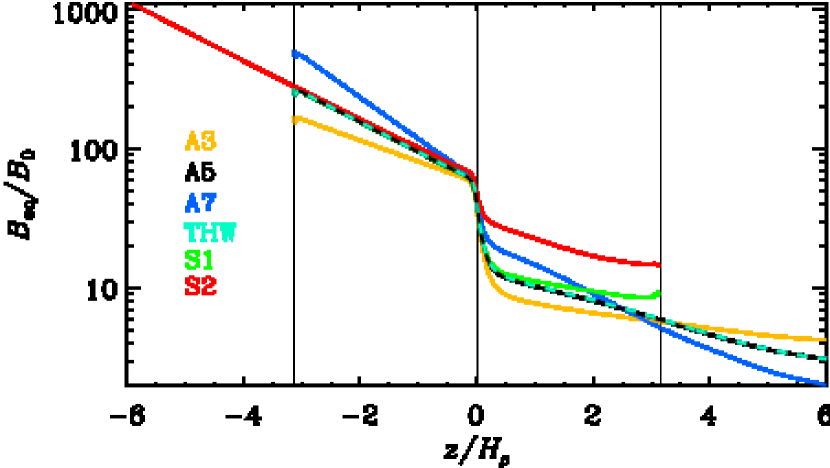
Figure 1: Vertical profiles of equipartition magnetic field strengths $B_{\rm eq}$ for Runs A3, A5, A7, THW, S1, and S2 as a function of height $z/H_{\rho}$. $B_{\rm eq}$ is normalized by the imposed magnetic field $B_{0}$. The vertical lines indicate $z=-\pi,\ 0,\ \pi$.

3 Results

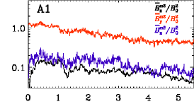
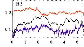
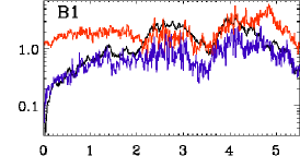
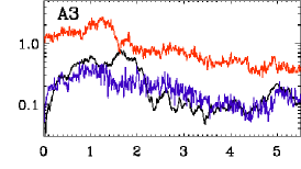
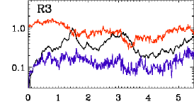
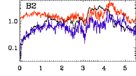
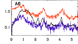
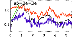
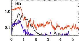
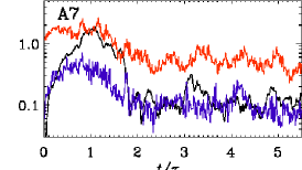
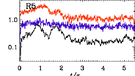
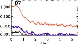
Figure 2: Temporal evolution of the horizontally averaged, magnetic energy density of the large-scale field at the surface ($z=0$) $\langle{\overline{\mbox{\boldmath$B$}}{}^{\rm fil\,2}}\rangle_{xy}$ for Sets A (first column), R (second column), and B (third column). The three components are shown in blue ($x$), red ($y$), and black ($z$). All values are normalized by the imposed field strength $B_{0}^{2}$. The straight green line in the panel for Run A5 shows the estimated growth rate of $1.4/\tau_{\rm td}$ for vertical large-scale magnetic field.

We comprehensively study the formation mechanism of the bipolar regions found in Warnecke et al. (2013b) by changing the density stratification, the magnetic Reynolds number, and the imposed magnetic field. For each parameter we perform five to eight runs in various sets: Set A for the density study, Set R for the magnetic Reynolds number study, and Set B for the imposed magnetic field study; see Table LABEL:runs. Furthermore, we use three different additional domain sizes to investigate their influence on the formation process; see Set S in Table LABEL:runs and two additional runs with vertical (Run V) and 45 degrees inclined (Run INC) imposed magnetic field.

The various stratifications and box sizes give rise to different vertical profiles of equipartition field strength $B_{\rm eq}$, which are plotted in Fig. 1. As a result of the transition from intense turbulence to small velocities in the coronal envelope, $B_{\rm eq}$ experiences a steep decrease at the surface ($z=0$).

We start by investigating the evolution of the magnetic field at the surface. We therefore calculate the averaged magnetic energy density of the large-scale field $\langle{\overline{\mbox{\boldmath$B$}}{}^{\rm fil\,2}}(z=0)\rangle_{xy}$; see Fig. 2 for all three components. Strong flux concentrations with high values for the large-scale magnetic field are obtained (see Table LABEL:runs) when the $z$ components (black lines) are similar or larger than the $y$ component (red), as in Runs A5, A6, A7, R3, B2, and B5. Furthermore, Fig. 2 shows a clear exponential growth of the large-scale vertical magnetic field in those cases where bipolar regions occur (compare with last column of Table LABEL:runs). This confirms that a hydromagnetic instability is responsible for the formation of the bipolar regions found in these simulations. In the second to last column of Table LABEL:runs, $\tilde{t}_{\rm max}=t_{\rm max}/\tau_{\rm td}$ is the time when $\overline{B}{}_{z}^{\rm fil\,max}$ is taken in terms of turbulent-diffusive time. In Set A, the formation of bipolar regions is connected to a growth of magnetic energies in all components, but the $z$ component grows exponentially during the first turbulent diffusion time for all runs, except Run A1. Our estimated growth rate for Run A5 is $1.4/\tau_{\rm td}$, which is plotted as a straight line in Fig. 2. This growth rate is well in agreement of earlier studies with imposed vertical and horizontal magnetic fields, i.e., those without a coronal envelope (Brandenburg et al. 2013; Kemel et al. 2012).

The $x$ component of $\langle{\overline{\mbox{\boldmath$B$}}{}^{\rm fil\,2}}(z=0)\rangle_{xy}$ also shows an exponential growth, but with a lower growth rate. In Set R, runs with both a lower and a higher magnetic Prandtl number than Run R4=A5 have a smaller growth rate, although Run R3 also shows bipolar regions. In Runs B1 and B2, there are also exponential increases of the energy of the vertical magnetic field, which are related to the formation of bipolar magnetic regions. These increases tend to occur later and have higher energies than Run A5. In Run B7, the vertical magnetic field is too weak to produce a magnetic flux concentration, as is also indicated by the lack of exponential growth. In the following, we study these behaviors in more detail.

3.1 Dependence on stratification

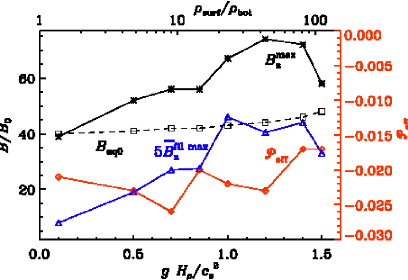
Figure 3: Dependence of magnetic field amplification and effective magnetic pressure on stratification. Maximum vertical magnetic field $B_{z}^{\rm max}/B_{0}$ (solid black) at the surface, maximum of the large-scale vertical magnetic field $5\overline{B}{}_{z}^{\rm fil\,max}/B_{0}$ (blue) at the surface, minimum of the effective magnetic pressure ${\cal P}_{\rm eff}$ (red), and equipartition field strength at the surface $B_{\rm eq0}/B_{0}$ (dashed black) as a function of $gH_{\rho}/c_{\rm s}^{2}$ and density contrast $\rho_{\rm surf}/\rho_{\rm bot}$ for Set A.

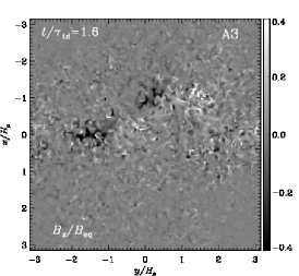
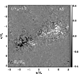
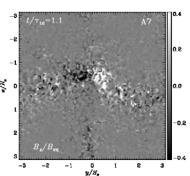
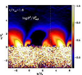
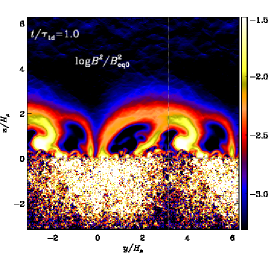
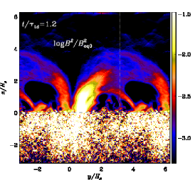
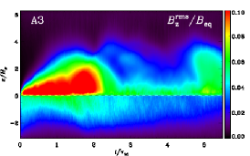
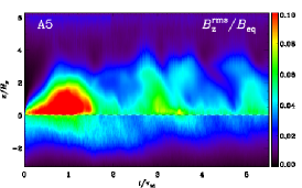
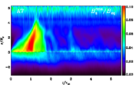
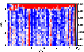
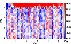
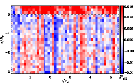
Figure 4: Formation of bipolar regions for three different stratifications (left column: A3, middle: A5, right: A7). Top row: normalized vertical magnetic field $B_{z}/B_{\rm eq}$ plotted at the $xy$ surface ($z=0$) at times when the bipolar regions are the clearest. Second row: normalized magnetic energy density plotted in the $yz$ plane as a vertical cut through the bipolar region at $x=0$. We replicated the domain by 50% in the $y$ direction (indicated by the vertical dashed lines) to give a more complete impression about spot separation and arch length. The black-white dashed lines indicate the replicated part and in the last three rows the surface ($z=0$). Third row: vertical rms magnetic field $B_{z}^{\rm rms}/B_{\rm eq}=\langle B_{z}^{2}\rangle_{xy}^{1/2}/B_{\rm eq}$ normalized by the local equipartition value (see Fig. 1 for vertical profiles) as a function of $t/\tau_{\rm td}$ and $z/H_{\rho}$. Bottom row: smoothed effective magnetic pressure ${\cal P}_{\rm eff}$ as a function of $t/\tau_{\rm td}$ and $z/H_{\rho}$. Blue shades correspond to negative and red to positive values.

In Runs A1–A8, we vary the density stratification in the turbulent layer from $\rho_{\rm bot}/\rho_{\rm surf}=1.5$ to $108$ by changing the normalized gravity $gH_{\rho}/c_{\rm s}^{2}$, where $\rho_{\rm bot}$ and $\rho_{\rm surf}$ are the horizontally averaged densities at the bottom ($z=-\pi$) and at the surface ($z=0$) of the domain, respectively. This is related to an overall stratification range from $\rho_{\rm bot}/\rho_{\rm top}=2.6$ (Run A1) to $1.2\times 10^{6}$ (Run A8), where $\rho_{\rm top}$ is the horizontally averaged density at the top of the domain ($z=2\pi$). The formation of a bipolar region depends strongly on the stratification. For a small density contrast, as in Run A1, the amplification of vertical magnetic field is too weak to form magnetic structures, its maximum is below the equipartition value at the surface; see Fig. 3. The vertical magnetic field in the flux concentrations can reach superequipartition field strengths and an amplification of over 50 of the imposed field strength already for a density contrast of $\rho_{\rm bot}/\rho_{\rm surf}\approx 5$, as in Run A2. However, the bipolar structures are still weak compared to those for higher stratifications. The field amplification inside the flux concentrations grows with increasing stratification. The maximal vertical field strength reaches values of over 70$B_{0}$, which is nearly twice the equipartition field strength at the surface. The maximum field strength peaks at $\rho_{\rm bot}/\rho_{\rm surf}=42$ and decreases for even higher stratification (Run A8). This limits strong field concentrations to a range between $\rho_{\rm bot}/\rho_{\rm surf}=23$ and $80$. Field concentrations are still possible for higher and lower stratifications, but the strengths of the large-scale field inside the bipolar region are smaller.

The density stratification also has an influence on the formation of the bipolar region. This is shown in the top row of Fig. 4, where we plot the vertical magnetic field strength at the surface at the time of strongest bipolar region formation. Run A3 with moderate stratification shows a magnetic field concentration that has multiple poles, and the structure of the bipole in Run A3 is not as clear as in Runs A5 and A7. In Run A7, the bipolar region is more coherent and magnetic spots are closer to each other than in Run A5. Furthermore, the maximum of the large-scale magnetic field $\overline{B}{}_{z}^{\rm fil\,max}/B_{0}$, which is an indication of the strength of bipolar regions, increases with higher stratification, as shown by the blue line in Fig. 3. A maximum of the large-scale magnetic field above about $5\,B_{0}$ seems to indicate bipolar flux concentrations. The inclination of the two polarities is most of the time aligned with the imposed field direction. However, in some cases, as in Run A5, an alignment with the surface diagonal is also possible. Unfortunately, we cannot find any clear criteria that determine the alignment.

In the second row of Fig. 4, we show how the magnetic field continues above the surface. Here we plotted $\log_{10}B^{2}/B_{\rm eq0}^{2}$ at a time when the bipolar regions are the clearest. The loop structures connecting the two polarities are more pronounced for high stratification (Run A7) than for moderate stratification (Run A3). Furthermore, in Runs A5 and A7, the magnetic energy in the turbulent region is much more concentrated and structured than in Run A3. These plots indicate that with higher stratification, it is easier to form loop-like structures in the coronal envelope. However, the inclination of the bipolar region as in Run A3 seems to form more complex loops structures than what is shown in Fig. 5 of Warnecke et al. (2013b).

In the third row of Fig. 4, we plot the horizontally averaged rms value of the vertical magnetic field $B_{z}^{\rm rms}=\langle B_{z}^{2}\rangle_{xy}^{1/2}$, which is normalized by the local equipartition value, as a function of time and height. In the coronal envelope, where turbulent forcing is absent, $B_{\rm eq}$ is much lower than in the turbulent layer; see Fig. 1 for the vertical profiles of $B_{\rm eq}$. This leads to high values of $B_{z}^{\rm rms}/B_{\rm eq}$ in the coronal envelope. We chose this normalization using $B_{\rm eq}$ instead of $B_{\rm eq0}$ because of the better visibility of the concentration of vertical flux. For all three cases, which are shown in the third row of Fig. 4, the field emerges from the turbulent layer, forming a bipolar region and then generating loop-like structures in the coronal envelope. After $t/\tau_{\rm td}\approx 2$, the vertical field decays, and new strong flux concentrations are not able to form. This is related to a persistent change of the average stratification after the magnetic field is applied.

An indicator of structure formation through the negative effective magnetic pressure instability (NEMPI) is the effective magnetic pressure ${\cal P}_{\rm eff}$. For its derivation, we start with the definition of the turbulent stress tensor $\Pi$, i.e.,

$$\Pi_{ij}^{(\overline{B})}\equiv\overline{\rho u^{\prime}_{i}u^{\prime}_{j}}+{\textstyle{1\over 2}}\delta_{ij}\mu_{0}^{-1}\overline{\mbox{\boldmath$b$}{}^{2}}-\mu_{0}^{-1}\overline{b_{i}b_{j}},$$ (7)

where the first term is the Reynolds stress tensor and the last two terms are the turbulent magnetic pressure and turbulent Maxwell stress tensors. The superscript $(\overline{B})$ indicates the turbulent stress tensor under the influence of the mean magnetic field; $\Pi_{ij}^{(0)}$ is the turbulent stress tensor without mean magnetic field, where both, the turbulent Maxwell stress and the Reynolds stress are free from the influence of the mean magnetic field. Here we define mean and fluctuations through horizontal averages, $\overline{}\mbox{\boldmath$B$}{}\equiv\langle\mbox{\boldmath$B$}{}\rangle_{xy}$, such that $\mbox{\boldmath$B$}{}=\overline{}\mbox{\boldmath$B$}{}+\mbox{\boldmath$b$}{}$ and $\mbox{\boldmath$u$}{}=\overline{}\mbox{\boldmath$U$}{}+\mbox{\boldmath$u$}{}^{\prime}$. Using symmetry arguments, we can express the difference in the turbulent stress tensor $\Pi$ for the magnetic and nonmagnetic case in terms of the mean magnetic field (see, e.g., Brandenburg et al. 2012),

$$\Delta\Pi_{ij}=\Pi_{ij}^{(B)}-\Pi_{ij}^{(0)}=-q_{p}\delta_{ij}{\overline{}\mbox{\boldmath$B$}{}^{2}\over 2}+q_{s}\overline{B}_{i}\overline{B}_{j}-q_{g}{g_{i}g_{j}\over g^{2}}\overline{}\mbox{\boldmath$B$}{}^{2},$$ (8)

where $q_{p}$, $q_{s}$, and $q_{g}$ are parameters expressing the importance of the mean-field magnetic pressure, mean-field magnetic stress, and vertical anisotropy caused by gravity. They are to be determined in direct numerical simulations: ${g_{i}}$ are components of $g$, which in our setup has only a component in the negative $z$ direction. The normalized effective magnetic pressure is then defined as

$${\cal P}_{\rm eff}=\frac{1}{2}(1-q_{p})\,\beta^{2},\quad{\rm with}\quad\beta^{2}={\overline{}\mbox{\boldmath$B$}{}^{2}\over B_{\rm eq}^{2}},$$ (9)

where we can calculate from Equation (8)

$$q_{p}=-{1\over\overline{}\mbox{\boldmath$B$}{}^{2}}\,\left(\Delta\Pi_{xx}+\Delta\Pi_{yy}-\left(\Delta\Pi_{xx}-\Delta\Pi_{yy}\right)\,{\overline{B}_{x}^{2}+\overline{B}_{y}^{2}\over\overline{B}_{x}^{2}-\overline{B}_{y}^{2}}\right),$$ (10)

$$q_{s}={\Delta\Pi_{xx}-\Delta\Pi_{yy}\over\overline{B}_{x}^{2}-\overline{B}_{y}^{2}},$$ (11)

$$q_{g}={1\over\overline{}\mbox{\boldmath$B$}{}^{2}}\,\left(-\Delta\Pi_{zz}-q_{p}{\overline{}\mbox{\boldmath$B$}{}^{2}\over 2}+q_{s}\overline{B}_{z}^{2}\right).$$ (12)

In the bottom row of Fig. 4, we show ${\cal P}_{\rm eff}$ for Runs A3, A5, and A7, where ${\cal P}_{\rm eff}$ was evaluated in $50\times 20$ bins in time and height within the turbulent layer. From these maps, we deduct the minimum values ${\cal P}_{\rm eff}^{\rm min}$ and list them in the ninth column of Table LABEL:runs; see also Figures 3, 7, and 9.

We find that the area with negative effective magnetic pressure ${\cal P}_{\rm eff}$ decreases for stronger stratifications (see the bottom row of Fig. 4). For Run A3, the smoothed ${\cal P}_{\rm eff}$ is negative in basically all of the turbulent layer at all times, except for some short time intervals. The values are often below $-0.005$, but occasionally even below $-0.01$. For higher stratification, the intervals of positive values of ${\cal P}_{\rm eff}$ become longer and negative values become in general weaker. In Run A7, the smoothed ${\cal P}_{\rm eff}$ fluctuates around zero with equal amounts of positive and negative values.

As ${\cal P}_{\rm eff}$ is plotted in the same time interval as $B_{z}^{\rm rms}$ (third row of Fig. 4), it enables us to compare the time evolutions of structure formation and ${\cal P}_{\rm eff}$. For Run A7, there seems to be a relation between the two, i.e., structure formation occurs when ${\cal P}_{\rm eff}$ is negative. When $B_{z}^{\rm rms}$ has a strong peak at around $t/\tau_{\rm td}\approx 1$, ${\cal P}_{\rm eff}$ has a minimum between $t/\tau_{\rm td}\approx 0.5$ and 1 close to the surface. In Runs A3 and A5, ${\cal P}_{\rm eff}$ is also weak when $B_{z}^{\rm rms}$ is strong, but this does not only happen when $B_{z}^{\rm rms}$ is strong. In general, the minimum value of the smoothened ${\cal P}_{\rm eff}$ does not indicate the existence of NEMPI as a possible formation mechanism of flux concentration in the context of dependency on density stratification. There is a weak opposite trend: ${\cal P}_{\rm eff}$ becomes less negative for large stratification, even though $\overline{B}{}_{z}^{\rm fil\,max}$ increases for larger stratification; see Fig. 3.

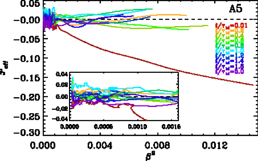
Figure 5: Effective magnetic pressure ${\cal P}_{\rm eff}$ plotted over $\beta^{2}=\overline{\mbox{\boldmath$B$}}{}^{2}/B_{\rm eq}^{2}$ at ten different times for Run A5. The inlay shows a zoom-in to the lower values of $\beta^{2}$, where we have averaged over 40 points to reduce the noise. The shown values are limited to the turbulent layer ($z\leq 0$).

Indeed, the value of ${\cal P}_{\rm eff}$ itself is not the decisive quantity, as the growth rate $\lambda$ of NEMPI is given by (Rogachevskii & Kleeorin 2007; Kemel et al. 2013; Brandenburg et al. 2014)

$$\lambda={v_{\rm A}\over H_{\rho}}\,\left(-2{{\rm d}{}{\cal P}_{\rm eff}\over{\rm d}{}\beta^{2}}\right)^{1/2}\,{k_{x}\over k}-\eta_{\rm t0}\,k^{2}.$$ (13)

See Appendix A of Kemel et al. (2013) for a detailed derivation with an imposed horizontal field, and Sect. 2.1 of Brandenburg et al. (2014) with a vertical field. Here $v_{\rm A}=B_{0}/\sqrt{\mu_{0}\rho}$ is the Alfvén speed. To get an idea about the form of ${\rm d}{}{\cal P}_{\rm eff}/{\rm d}{}\beta^{2}$, we plot in Fig. 5 ${\cal P}_{\rm eff}$ versus $\beta^{2}=\overline{\mbox{\boldmath$B$}}{}^{2}/B_{\rm eq}^{2}$ at different times for Run A5. In the beginning of the simulation, the growth rate is positive for all values of $\beta^{2}$ in the turbulent layer because the derivative, ${\rm d}{}{\cal P}_{\rm eff}/{\rm d}{}\beta^{2}$ is negative. As the simulation progresses, the growth rate become weaker and mainly at larger values of $\beta^{2}$ it is positive. After the formation of the largest and strongest concentrations at around $t/\tau_{\rm td}=\tilde{t}_{\rm max}=1.0$ (light blue), the growth rate is positive only at low values of $\beta^{2}$, as shown in the inlay of Fig. 5. However, even when the growth rate is positive, the actual values of ${\cal P}_{\rm eff}$ are still positive. This behavior of the growth rate fits well with the temporal evolution of the large-scale magnetic field as shown in Fig. 2. There, $\langle{\overline{\mbox{\boldmath$B$}}{}^{\rm fil\,2}}\rangle_{xy}$ exhibits an exponential growth until around $t/\tau_{\rm td}=1.0$, saturates and then decays after $t/\tau_{\rm td}=1.2$. At low values of $\beta^{2}$, ${\cal P}_{\rm eff}$ does not show a strong indication of a negative slope; it seems nearly constant and the growth rate is close to zero; see inlay of Fig. 5.

We should note here that the mean field $\overline{\mbox{\boldmath$B$}}{}$ is in the direction of the imposed magnetic field, i.e., the $y$ direction, while the field in the spots points in the positive or negative $z$ direction. Therefore, besides the usual formation of concentrations with the same polarity as the imposed field, we have here an additional mechanism to turn the field from horizontal to vertical. One of these mechanisms can be magnetic buoyancy (e.g., Parker 1955b), which is actually visible in Fig. 5, where ${\rm d}{}{\cal P}_{\rm eff}/{\rm d}{}\beta^{2}$ becomes positive. Even though it is not easy to determine the growth rate for the simulations, we can get a rough idea by looking at $\tilde{t}_{\rm max}$ for increasing stratification. Interestingly, $\tilde{t}_{\rm max}$ tends to decrease, implying a stronger growth rate for larger stratification.

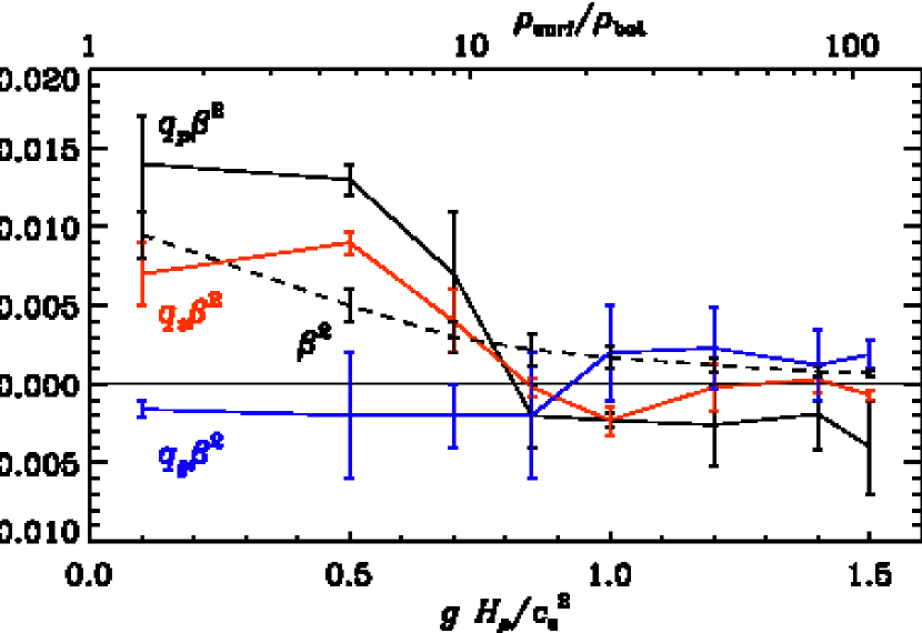
Figure 6: Dependence of parameters $q_{p}$ (black), $q_{s}$ (red), and $q_{g}$ (blue) on stratification for Set A. We normalize the parameters by multiplying with $\beta^{2}$ (dashed black). The legend of the x-axis is the same as in Fig. 3. The parameters are computed as a temporal and spatial mean over the turbulent layer. Error bars are estimated using the maximum difference of the total mean with the means of each third of the time series.

To understand the dependence on stratification, we analyze the three parameters in the three terms of Equation (8) defined in Equations (10)–(12). They quantify the importance of the different contributions to the turbulent stress tensor $\Pi$. In Fig. 6, we plot the parameters $q_{p}$, $q_{s}$, and $q_{g}$ as functions of density stratification. The errors are relatively large because the parameters are strongly fluctuating in time and space. Nevertheless, there are some systematic trends with increasing density stratification. The parameter $q_{p}\beta^{2}$ is related to ${\cal P}_{\rm eff}$ and shows a strong decrease from low to moderate stratifications ($\rho_{\rm bot}/\rho_{\rm surf}<15$), and it is even larger than the decrease in $\beta^{2}$ itself. This means, the average ${\cal P}_{\rm eff}$ is only negative for $\rho_{\rm bot}/\rho_{\rm surf}$ smaller than $\approx 15$. For larger stratifications, ${\cal P}_{\rm eff}$ is on average positive. However, this also means that, as shown in the last row of Fig. 4, ${\cal P}_{\rm eff}$ can be negative at certain times and certain depths. The parameter $q_{g}$, describing vertical anisotropy due to gravity, is negative for low and moderate stratifications and becomes positive for high stratification showing a steady increase. Therefore, $q_{g}\beta^{2}>\beta^{2}$ can also decrease the turbulent pressure, which is the trace of $\Pi$. This seems to be the case at least on average for high stratifications ($\rho_{\rm bot}/\rho_{\rm surf}>20$). However, because of the direction of the gravity, only $\Pi_{zz}$ is suppressed. This might be related to the fact that we still find bipolar regions for high stratification, but the field strength is weaker than for moderate stratifications. This behavior might explain the “gravitational quenching” found by Jabbari et al. (2014). The coefficient $q_{s}$, characterizing the importance of the off-diagonal components of the turbulent stress tensor, does not seem to have a strong influence on the result. Furthermore, the sign is positive for low stratifications, close to zero for higher stratifications, and therefore $q_{s}\beta^{2}<\beta^{2}$ for most of the runs. Thus, the $q_{s}$ terms could only suppress the turbulent pressure if the components of the magnetic stress tensor themselves were negative. The averaged coefficients $q_{p}$, $q_{s}$, and $q_{g}$ indicate that the main mechanism for flux concentration for low and moderate stratifications ($\rho_{\rm bot}/\rho_{\rm surf}\leq 15$) is related to the negative effective magnetic pressure ${\cal P}_{\rm eff}$, whereas for high stratifications ($\rho_{\rm bot}/\rho_{\rm surf}\geq 15$), the contribution of the vertical anisotropy due to gravity is more important. However, as discussed before, the averaged quantities are strongly affected by fluctuations. Comparing our values with previous works (Brandenburg et al. 2012; Käpylä et al. 2012a), we find broad agreement. In Brandenburg et al. (2012), $q_{g}\beta^{2}$ is smaller and positive for similar stratification, while $q_{s}\beta^{2}$ is close to zero. In the present work $q_{p}$ is negative instead of positive for the same stratification. In Käpylä et al. (2012a), where turbulent convection is considered instead of forced turbulence, $q_{g}$ turns out to be positive and $q_{s}$ negative, which is similar to our simulations with similar stratification. A detailed comparison with Warnecke et al. (2013b) reveals that the structure of the bipolar region and its $\tilde{t}_{\rm max}$ of case A is not exactly the same as in Run A5, even though the only difference is the resolution and precision. This suggests that in the simulations of Warnecke et al. (2013b) the resolution was not sufficient to model this highly turbulent medium.

In addition to the change in stratification, we also change the forcing width from $w=0.05$ to $w=0.02$ in one case (Run THW). The resulting change in the vertical profile of the equipartition field strength is small, as shown in Fig. 1. The resulting bipolar regions, however, are slightly weaker, $B_{z}^{\rm max}/B_{0}=56$, and the large-scale field is significantly weaker than in Run A5. This might also be related to the fact that the $B_{\rm eq0}$ is slightly higher. Thus, in summary, the forcing width does not have a strong influence on the occurrence of bipolar regions.

3.2 Dependence on magnetic Reynolds number

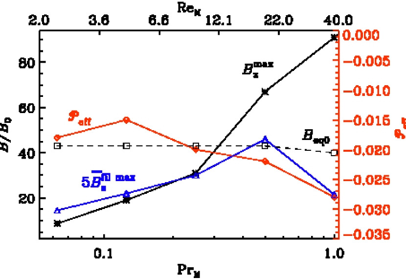
Figure 7: Dependence of magnetic field amplification and effective magnetic pressure on magnetic Prandtl number $\mbox{\rm Pr}_{\rm M}$ and magnetic Reynolds number $\mbox{\rm Re}_{\rm M}$ for Set R. The legend is otherwise the same as in Fig. 3.

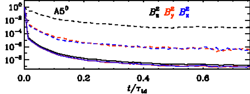
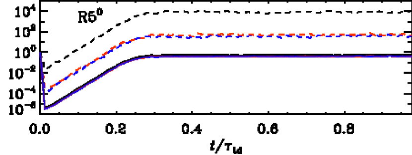
Figure 8: Temporal evolution of the horizontally averaged magnetic energy density at the surface ($z=0$) for Runs A5⁰ and R5⁰, where $B_{0}=0$. The three components are shown in blue ($x$), red ($y$), and black ($z$), where solid lines indicate the total magnetic energy and dashed lines the large-scale magnetic energy. All values are normalized by their values at $t/\tau_{\rm td}=0$.

As a next step we investigate the dependency on magnetic Reynolds number $\mbox{\rm Re}_{\rm M}$. We keep Re fixed (around 40) and change $\mbox{\rm Pr}_{\rm M}$ by a factor of 16; see the seventh column in Table LABEL:runs. Run R1, has the lowest $\mbox{\rm Pr}_{\rm M}$ and a magnetic Reynolds number of $\mbox{\rm Re}_{\rm M}=2.4$. This implies that microscopic diffusion is of the same order as turbulent diffusion. The effect of negative magnetic pressure is weak for such low magnetic Reynolds numbers. Indeed, the maximum amplification of the magnetic field due to the flux concentration is around 5, which is nearly ten times less than the equipartition value. Also the amplification of the large-scale magnetic field is weak. Even though the minimum value of ${\cal P}_{\rm eff}$ is similar to those of Set A, NEMPI cannot be excited, presumably because the growth rate of NEMPI is smaller than the damping rate caused by turbulent and microscopic magnetic diffusion.

Increasing $\mbox{\rm Re}_{\rm M}$ and $\mbox{\rm Pr}_{\rm M}$ leads to larger field amplifications and stronger large-scale fields inside the flux concentrations; see Figs. 2 and 7. However, the vertical field can only reach superequipartition values when $\mbox{\rm Pr}_{\rm M}$ is above 0.5. The dependence on $\mbox{\rm Re}_{\rm M}$ can also be seen from the time $\tilde{t}_{\rm max}$ (time instant when $\overline{B}{}_{z}^{\rm fil\,max}$ is reached). Increasing $\mbox{\rm Re}_{\rm M}$ leads to a shorter $\tilde{t}_{\rm max}$, but in Run R5, the instability is weakened and causes $\tilde{t}_{\rm max}$ to be longer. This behavior can also be seen in the evolution of the components of the magnetic energy; see Fig. 2. For $\mbox{\rm Pr}_{\rm M}\leq 1$, the growth becomes steeper with increasing $\mbox{\rm Pr}_{\rm M}$ until the maximum is reached for Run A5=R4. For $\mbox{\rm Pr}_{\rm M}=0.5$, i.e., for Run R5, the growth rate is again smaller than for Run A5=R4.

In Run R5, the magnetic Prandtl number is unity and a small-scale dynamo is excited. This is illustrated in Fig. 8, where we plot the $x$, $y$, and $z$ components of the magnetic energy as a function of $t/\tau_{\rm td}$ for Runs A5⁰ and R5⁰. These two simulations are identical to Runs A5 and R5, except that we set the imposed field $B_{0}$ to zero and use a weak, white-noise seed magnetic field instead. For Run A5⁰ all components of the magnetic field decay as expected because NEMPI needs a small imposed mean magnetic field to operate. In Run R5⁰ a small-scale dynamo operates and generates magnetic field in all components, but their rms values stay constant after exponential amplification. Even though the magnetic field amplification is maximal in Run R5, small-scale dynamo action weakens the formation of large-scale vertical magnetic structures. Earlier work (Brandenburg et al. 2012) demonstrated that the relevant mean-field parameter proportional to the growth rate is reduced to 2/3 of it original value when $\mbox{\rm Re}_{\rm M}>60$. Therefore, $\overline{B}{}_{z}^{\rm fil\,max}$ is smaller than in Run R4 and the bipolar magnetic region is weaker. On the other hand, ${\cal P}_{\rm eff}$ is actually more negative than in Run R4. The magnetic field produced by the small-scale dynamo reduces $u_{\rm rms}$ and, therefore, Re and $B_{\rm eq0}$ also .

In the Sun, the fluid and magnetic Reynolds numbers are expected to be very large, allowing therefore a small-scale dynamo to operate even though the magnetic Prandtl number might be small (see, e.g., Brandenburg 2011; Rempel 2014). This might weaken the formation of bipolar regions due to NEMPI in the Sun, but large Re and $\mbox{\rm Re}_{\rm M}$ could also enhance the NEMPI growth rate due to lower diffusion. However, a reliable extrapolation of the interaction of NEMPI and the small-scale dynamo is not possible at the moment, as the simulations of both NEMPI and small-scale dynamo are still operating in a regime that is too diffusive compared with the Sun.

3.3 Dependence on imposed magnetic field strength

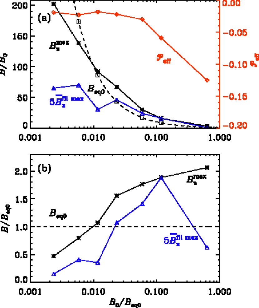
Figure 9: Dependence of magnetic field amplification and effective magnetic pressure on the imposed magnetic field $B_{0}/B_{\rm eq0}$ for Set B. The magnetic field is normalized by the imposed magnetic field $B_{0}$ (a) or by the equipartition field strength at the surface $B_{\rm eq0}$ (b). Otherwise the legend is the same as in Fig. 3.

In the runs of Warnecke et al. (2013b) and in all runs of Sets A, R, and S, we impose a weak horizontal magnetic field. The strength of this field is less than $1/40$ of the equipartition field strength at the surface, i.e., the ratio between it and the equipartition field strength is more than $1/200$ at the bottom of the domain in the case of Run A5. To investigate the dependence on the imposed magnetic field strength, we vary the imposed field in the runs of Set B from $B_{0}/B_{\rm eq0}=1/430$ to 2/3; see the eighth column in Table LABEL:runs. In Fig. 9, we show the dependence of the magnetic field and ${\cal P}_{\rm eff}$ on $B_{0}/B_{\rm eq0}$. In Run B1, where $B_{0}$ is weak, the field strength is high enough to serve as an initial magnetic field for NEMPI to work, but only weak flux concentrations are formed. Therefore the field amplification is around two times smaller than the equipartition field strengths. The large-scale field is even more than 30 times lower than the equipartition field, therefore, preventing the formation of high flux concentrations. However, here the large-scale magnetic energy also shows an exponential growth; see Fig. 2. In Run B2, the imposed field strength is sufficient to form bipolar magnetic regions, even though the maximum vertical field strength is just below the equipartition field strength. An increase of the imposed field leads to a stronger magnetic field inside the flux concentration compared with $B_{\rm eq0}$, see Fig. 9(b), but weaker fields compared to the imposed magnetic field; see Fig. 9(a). This is plausible: if a weak field is imposed, just a small fraction of the turbulent energy is used to concentrate and amplify the field to higher field strength. This leads to a high ratio of $B_{z}^{\rm max}/B_{0}$, but to a low ratio of $B_{z}^{\rm max}/B_{\rm eq0}$. In Run B6, where the imposed field is strong, a small concentration and amplification of $B_{z}^{\rm max}/B_{0}=16$ can lead to strong superequipartition field strengths of $B_{z}^{\rm max}/B_{\rm eq0}=1.9$. For a strong imposed magnetic field, when the derivative ${\rm d}{}{\cal P}_{\rm eff}/{\rm d}{}\beta^{2}$ becomes positive, NEMPI cannot be excited and magnetic spots are not expected to form (Kemel et al. 2013). In particular, in Run B7 the magnetic field becomes too strong, so no bipolar magnetic region can be built up. This leads us to conclude that there is an optimal imposed field strength, which is between $B_{0}/B_{\rm eq0}=0.012$ and $0.12,$ when superequipartition magnetic flux concentrations and bipolar magnetic structures can be formed.

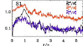
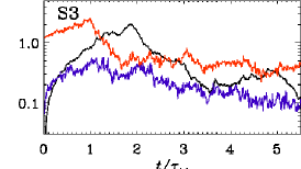
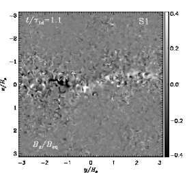
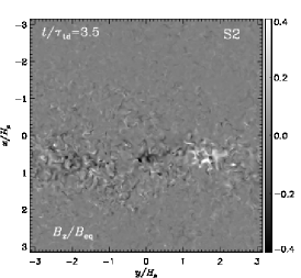
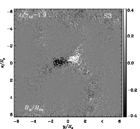
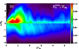
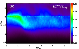
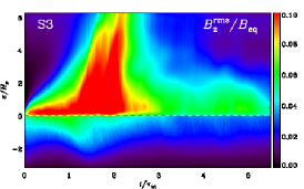
Figure 10: Formation of bipolar regions for three different sizes (left column: S1, middle: S2, right: S3). Top row: the same as in Fig. 2, but for Set S. Middle row: normalized vertical magnetic field $B_{z}/B_{\rm eq}$ plotted at the $xy$ surface ($z=0$) at times, when the bipolar regions are the clearest. Bottom row: vertical rms magnetic field $B_{z}^{\rm rms}/B_{\rm eq}=\langle B_{z}^{2}\rangle_{xy}^{1/2}/B_{\rm eq}$ normalized by the local equipartition value as a function of time $t/\tau_{\rm td}$ and height $z$. The black-white dashed line in the bottom row marks the surface ($z=0$).

As expected, the effective magnetic pressure ${\cal P}_{\rm eff}$ decreases as we increase the magnetic field, except in Run B1, where it is slightly smaller than in Run B2, see Fig. 9(a). Furthermore, $\tilde{t}_{\rm max}$ shows a dependence on the imposed field. For stronger imposed fields, $\tilde{t}_{\rm max}$ becomes shorter, indicating a higher growth rate of the instability as seen in the steeper growth in Fig. 2. However, this seems to be only true for strong concentrations; the weak concentrations in Run B1 have a smaller $\tilde{t}_{\rm max}$ than those in Run B2. This is probably related to the two distinct growth rates seen in the magnetic energy of Fig. 2. Furthermore, a stronger magnetic field suppresses turbulent motions, as seen from the decrease of Re (sixth column of Table LABEL:runs) and therefore it decreases the turbulent magnetic diffusivity. This influences the values of $\tau_{\rm td}$ and, therefore, $\tilde{t}_{\rm max}$, but also allows for a higher growth rate.

3.4 Dependence on box size

To investigate how the formation of bipolar regions of Warnecke et al. (2013b) and in the present work depends on the chosen box size, we change the vertical size as well as the horizontal size; see Set S in Table LABEL:runs. In Fig. 10, we plot, for all cases of Set S, the magnetic energy of all three components in the large-scale field (top row), the vertical magnetic field at the time of clearest formation of bipolar structures (middle row), and the evolution of the vertical rms magnetic fields as functions of time and height (bottom row). In Run S1, we reduce the vertical size of the coronal envelope from $2\pi$ to $\pi$ keeping the other sizes the same; see Fig. 1 for the vertical profile of $B_{\rm eq}$. This change has only a small effect on the formation of bipolar regions. Comparing Run S1 with Run A5, $B_{z}^{\rm max}/B_{0}$ is reduced from 67 to 52 in Run A5 and the large-scale field $\overline{B}{}_{z}^{\rm fil\,max}/B_{0}$ from 9.2 to 7.8, whereas the value of $\tilde{t}_{\rm max}$ stays nearly the same. The structure of the bipolar regions is similar, but these regions seem to be more concentrated in Run A5.

As a second case (Run S2), we use the setup of Run S1 and extend the height of the turbulent layer from $\pi$ to $2\pi$. The value of the density at the surface stays the same, so the stratification extends to higher values of density in the lower layers. Also, the density contrast changes accordingly from 23 in the turbulent layer with a vertical extension of $\pi$ to 512 with a vertical extension of $2\pi$. This leads to a small increase of $u_{\rm rms}$ and, therefore, to a corresponding slight increase of $B_{\rm eq0}$; see Fig. 1. The maximal field amplification of $B_{z}^{\rm max}/B_{0}$ inside the flux concentration is higher than in Run S1, but still lower than in Run A5. The maximum of the large-scale magnetic field $\overline{B}{}_{z}^{\rm fil\,max}/B_{0}$ is half as low as in Runs S1 and A5. The bipolar regions are weaker and are more diffused. As can be seen in the bottom row of Fig. 10, only a weak concentration of vertical magnetic field is observed.

As a third case (Run S3), we extend the horizontal size of the box from $2\pi\times 2\pi$ to $4\pi\times 4\pi$; otherwise the setup of the run is the same as Run A5. In the top row of Fig. 10, we already see a strong excess of vertical magnetic energy in the large-scale field compared to the horizontal components with a maximum around $t/\tau_{\rm td}=2$. Indeed, this behavior can also be found by looking at the maximum of the vertical magnetic field and the large-scale vertical magnetic field at the surface; see Table LABEL:runs. $B_{z}^{\rm max}/B_{0}$ is much higher than in Run A5, and $\overline{B}{}_{z}^{\rm fil\,max}/B_{0}$ reaches higher values than in all other runs. The vertical magnetic field at the surface shows a clear bipolar region with well-concentrated poles. The size of the bipolar region is comparable with the size in the other runs and, therefore, it is independent of the horizontal size of the domain. The strong concentration of vertical magnetic field causes a strong response in the coronal envelope. In a box with twice the horizontal extent, the magnetic energy is four times larger than that of the imposed magnetic field. The more magnetic energy becomes available, the more magnetic flux can be concentrated. This also means, that the instability operating in these simulations is more efficient to concentrate flux in the horizontal direction than in the vertical direction, as seen in Run S2. In all three cases, the formation of bipolar regions can be associated with an exponential growth of the large-scale vertical magnetic energy, as seen from the top row of Fig. 10. Their growth rates are similar, but the resulting formation is different. Run S3 exhibits the strongest large-scale magnetic field of all simulations with a horizontal imposed field, but the growth rate is smaller than in Run A5. However, the duration of exponential growth in Run S1 is twice that of Run A5, allowing the field to grow to much higher values than in Run A5.

3.5 Dependence on field inclination

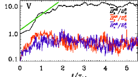
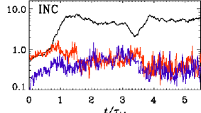
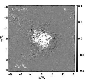
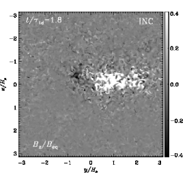
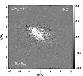
Figure 11: Formation of bipolar regions for two different field inclinations, left-hand side with purely vertical field (Run V) and right-hand side with y-z inclination (Run INC). Top row: the same as in Fig. 2, but for Runs V and INC. The straight green line for Run V illustrates the exponential growth of the energy in the vertical large-scale magnetic field. Bottom row: normalized vertical magnetic field $B_{z}/B_{\rm eq}$ plotted at the $xy$ surface ($z=0$) at times when the bipolar regions are the clearest. Run INC is shown for an early time ($t/\tau_{\rm td}=1.8$) and a later time ($t/\tau_{\rm td}=4.0$) to illustrate the change from a bipolar to monopolar structure.

In all of the runs mentioned above, we imposed a horizontal magnetic field. This leads to the formation of bipolar regions. In this subsection, we also study the cases of an imposed vertical and inclined field. For the vertical field (Run V), we set $\mbox{\boldmath$B$}{}_{\rm imp}=(0,0,B_{0})$ with the same field strengths and the same hydrodynamic quantities as in Run A5. As a result, the instability produces a single magnetic spot instead of a bipolar region. Because the magnetic energy is now concentrated in one single spot, the maximum magnetic field reaches nearly two times the values of Run A5 and more than two times the equipartition field strength. The field strength in the large-scale field is even three times stronger than in Run A5; see Table LABEL:runs. In the bottom row of Fig. 11, we plot the vertical magnetic field at the surface at the time of the clearest appearance. The single spot has a larger spatial extension and is more concentrated as in Run A5. Also here, we can find an exponential growth of the magnetic energy in the vertical field, as shown in top row of Fig. 11. We estimate the growth rate to be around $0.7/\tau_{\rm td}$, which is two times lower than for Run A5. Even though the growth rate is smaller than in Run A5, the duration is longer than in Run A5, leading to a stronger magnetic field. Also, the vertical field has already increased from a strength of $B_{0}$ in Run V, whereas in Run A5 there is no vertical magnetic field in the beginning of the simulation. An additional difference from Run A5 is that the spot does not decay after some time. Instead it stays roughly the same after $t/\tau_{\rm td}=2$.

Similar singular spots were already found by Brandenburg et al. (2013). There, the authors use a similar model with imposed vertical magnetic field, except their turbulent layer has a vertical extension of $2\pi$ instead of $\pi$ and no coronal envelope. In the runs of Brandenburg et al. (2013), where they use the same imposed field strengths, the maximum of the field strength is also more than double, and $\overline{B}{}_{z}^{\rm fil\,max}$ is close to the equipartition field strength at the surface. However, looking at their Fig. 2, the large-scale magnetic field grows exponentially up to $t/\tau_{\rm td}=1.5$ when the saturation set slowly in, whereas in our Run V the saturation sets in a bit later in time, $t/\tau_{\rm td}=2$. Nevertheless, our estimated growth rate of about $0.7/\tau_{\rm td}$ is half the value found in Brandenburg et al. (2013).

As a second case (Run INC), we impose an $yz$ inclined magnetic field with the strength of $B_{0}$ ($\mbox{\boldmath$B$}{}_{\rm imp}=(0,B_{0},B_{0})/\sqrt{2}$). As expected, we find the generation of a weak negative and a strong positive polarity in the bipolar region, as shown in the lower row of Fig. 11. However, this is only the case in the first half of the simulation. Then the weak negative polarity reconnects with the stronger positive polarity to form a single spot that does not diffuse away, which is similar to Run V. Because of the field reconnection, the resulting single spot is weaker than in Run V; see bottom row of Fig. 11. This behavior can be also seen in the evolution of the three components of the large-scale magnetic energy; see top row of Fig. 11. Until $t/\tau_{\rm td}=0.8,$ the $y$ and $z$ components grow exponentially with a similar growth rate, but then the $z$ energy component increases the growth rate that is properly related to the emergence of horizontal flux to form vertical flux. At $t/\tau_{\rm td}=1.8$, nearly at the end of the exponential growth stage, a weak negative and a strong positive pole form. At the $t/\tau_{\rm td}=3.5-3.8$, after a decrease of all components, only the vertical field recovers. This coincides with the diffusion of the weak negative spot. The behavior of an inclined field is exactly that can be expected from the two cases with imposed horizontal and vertical fields. For the horizontal field, a bipolar region is formed, which decays after several turbulent-diffusive times. For the vertical field, a single spot is formed, which does not diffuse.

3.6 Formation mechanism

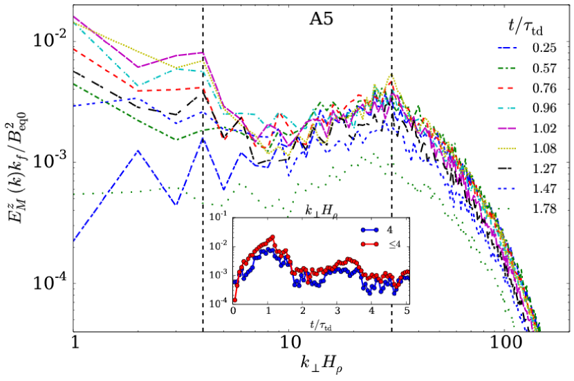
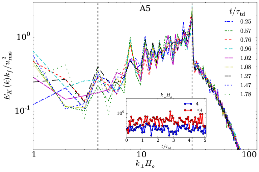
Figure 12: Magnetic and kinetic power spectrum for Run A5. Top panel: spectrum of vertical magnetic energy $E^{z}_{\rm M}$ at nine different times around $\tilde{t}_{\rm max}$ at the surface ($z=0$) as a function of horizontal wavenumber $k_{\bot}$. The inlay shows the vertical energy at $k_{\bot}H_{\rho}=4$ (blue line) and $k_{\bot}H_{\rho}\leq 4$ (red) as a function of time $t/\tau_{\rm td}$. Bottom panel: spectrum of the kinetic energy $E_{\rm K}$ plotted the same as the top panel. The vertical dashed lines indicate $k_{\bot}H_{\rho}=4$ and $k_{\bot}H_{\rho}=k_{\rm f}H_{\rho}=30$.

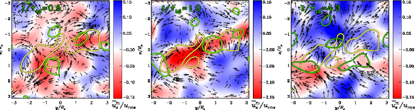
Figure 13: All three large-scale velocity components $\overline{u}_{x}^{\rm fil}$, $\overline{u}_{y}^{\rm fil}$, and $\overline{u}_{z}^{\rm fil}$ before ($t/\tau_{\rm td}=0.5$), at ($t/\tau_{\rm td}=1.0$), and after ($t/\tau_{\rm td}=4.3$) the occurrence of the bipolar regions (compare with Fig. 4) in the $xy$ plane for Run A5. The vertical velocity is plotted as red (downflows) and blue (upflows) and are normalized by the $u_{\rm rms}$ in the bulk of the turbulent layer ($z\leq 0$). The horizontal components of the velocity field are shown as arrows, where the lengths corresponds to the strength of the flow. Additionally, the contours of negative horizontal divergence is plotted in green for all three times. The yellow contours in all plots show the magnetic field at the time ($t/\tau_{\rm td}=1.0$) to guide the eye to the location of the bipolar region formation.

We also investigate in this context the formation mechanism leading to bipolar regions in the two-layer setup of stratified turbulence. As discussed in Warnecke et al. (2013b), the coronal envelope plays an important role in the formation process. However, the magnetic field, which gets concentrated, comes from the turbulent layer. This is shown with the two runs in Warnecke et al. (2013b), where one is the same setup as Run A5 of this work and one does not have any imposed field in the coronal envelope. Both show flux concentrations of similar strength. We also compare Runs A5 and S1, where the only difference lies in the size of the coronal envelope. Both show similar field concentrations, where $\overline{B}{}_{z}^{\rm fil\,max}/B_{0}$ has nearly the same value. Therefore, the size of the coronal envelope does not seem to have a strong influence on large-scale magnetic field and the formation of bipolar regions.

In the beginning of the simulation, the magnetic field is uniformly oriented in the $y$ direction because of the imposed field. The tangling of the magnetic field by turbulence also leads to field components in the other directions in the turbulent layer. This can been seen in Fig. 2 for most of the runs. Furthermore, we can use the plots of $B_{z}^{\rm rms}/B_{0}$ in Figs. 4 and 10 to analyze the height distribution of the vertical magnetic field in the formation process. The vertical field is built up in nearly the entire turbulent layer, which is in particular visible for Runs A3 and A5 as blue shades at early times. Then this vertical field gets concentrated and transported toward the surface, as shown by the increase of dark purple shades in the turbulent layer from the bottom toward the surface. This field evolves rapidly and leads to a flux concentration at the surface, which is visible as red shades. This vertical magnetic field then rises through the coronal layer until it decays and falls back toward the turbulent layer. Also, in the turbulent layer the field is first concentrated toward the surface, reaching the strongest peak of magnetic field and then the field diffuses back into the turbulent layer. These plots show clearly that the magnetic field originates from the turbulent layer toward the surface and does not come from the coronal envelope. A little later, after the peak of vertical flux has dissolved, the magnetic field from the coronal envelope falls toward the turbulent layer. The coronal envelope is important, but mostly as a free boundary condition for the magnetic field and the flow.

To illustrate how the magnetic and kinetic energies evolve at different scales, we plot in Fig. 12 the spectrum of the energy in the vertical magnetic field as well as the kinetic energy for Run A5 for nine different times. In both spectra, the normalized forcing wavenumber $k_{\rm f}H_{\rho}$ is seen as a local maximum. In the magnetic spectrum, the forcing scale has the highest peak in the beginning of the simulation. Later, more and more energy is transported to larger scales ($k_{\bot}H_{\rho}<10$) until the energy for $k_{\bot}H_{\rho}<5$ becomes dominant. This happens when $t\approx\tau_{\rm td}$, which is not surprisingly at the same time, when the bipolar region is the strongest ($t/\tau=\tilde{t}_{\rm max}$). Afterward, the magnetic energy decays first at larger scales and then at all scales. This can also be seen in the inlay, where we plot the energy of the vertical magnetic field at $k_{\bot}H_{\rho}=4$ (blue) and $k_{\bot}H_{\rho}\leq 4$ (red). There is a strong growth up to $t/\tau_{\rm td}=1$ and a decay to slower values after that. This means that the instability occurring in these simulations transports vertical magnetic energy to large scales in the growing phase. This has also been seen in previous studies with imposed vertical magnetic field (Brandenburg et al. 2014) and seems to be analogous to the inverse magnetic helicity cascade (Pouquet et al. 1976; Brandenburg 2001). It suggests the use of a cutoff wavenumber of $k_{\rm c}\leq k_{\rm f}/6$ to represent the large scales of the magnetic field in our previous analysis; see also Brandenburg et al. (2014) for a similar discussion. In the kinetic spectrum, the forcing scale is the highest peak for all times. There the energy of large scales are significant lower than those of the forcing scale. The kinetic energies on the larger scale show no strong time evolution, we only notice a small increase in time at $k_{\bot}H_{\rho}\leq 2$.

To study the influence of the forcing scale, we perform one additional run (Run F), where we decrease $k_{\rm f}$ from $30\,k_{1}$ to $15\,k_{1}$. As shown in the last row of Table LABEL:runs, the maximum vertical magnetic field strength is lower and the maximum of the large-scale vertical field is slightly larger than in Run A4. However, reducing the forcing wavenumber by half has almost no effect on the structure formation of bipolar regions via NEMPI. This confirms the results of previous studies of Brandenburg et al. (2014), where no strong dependence was found either. Even for significantly smaller forcing scales, flux concentrations were obtained when increasing the imposed field strength. From the theoretical side, the forcing scale should have an influence on the growth rate as well as on the turbulent magnetic diffusivity. A detailed study of the dependence of bipolar regions formation on the forcing scale is currently beyond the scope of this paper.

As found by Brandenburg et al. (2014), flux concentrations due to NEMPI show clear signatures of downflow patterns along the vertical magnetic field. Before and during the concentration of vertical flux, there exist strong converging downflows. Testing whether the bipolar magnetic region found in both Warnecke et al. (2013b) and in the present work also coincides with such a flow pattern; we show in Fig. 13 the large-scale velocity at the surface for the time before ($t/\tau_{\rm td}=0.5$), at ($t/\tau_{\rm td}=1.0$), and after ($t/\tau_{\rm td}=4.0$) the time of the strongest flux concentration for Run A5. For this we calculate the large-scale velocity with 2D horizontal Fourier filtering $\overline{}\mbox{\boldmath$u$}{}{}^{\rm fil}$ to exclude the velocities due to forcing. We use the technique described in Section 2 with a cutoff wavenumber of $k_{\rm c}\leq k_{\rm f}/6$. The flows are shown together with the large-scale magnetic energy and the horizontal divergence of the large-scale flow ($\partial_{x}\overline{u}_{x}{}^{\rm fil}+\partial_{y}\overline{u}_{y}{}^{\rm fil}$). At $t/\tau_{\rm td}=0.5$, before the bipolar region has appeared, and we find strong downflows (red) and horizontal converging flows in the vicinity where the bipolar region later forms (yellow contours). In the proximity of the downflows, there are also regions of negative horizontal divergence (green contours). At the time of the clearest appearance of the bipolar region ($t/\tau_{\rm td}=1.0$), the large-scale downflows are exactly at the location of strong magnetic energy, indicating a tight connection between the downflows and the formation of bipolar regions. Furthermore, we find a strong horizontal flow streaming into the region of large magnetic energy together with negative values of horizontal divergence. After the decay of the bipolar region ($t/\tau_{\rm td}=4.3$), the downflows are much weaker and upflows seem to dominate the large-scale vertical velocities. In the region where the magnetic field was previously strong, we do not observe strong concentrations of converging flows.

It is important to note here that all flow structures shown in Fig. 13 are at scales larger than the forcing scale and would not form owing to forced stratified turbulence alone. In the simulations without an imposed magnetic field, these flow patterns do not appear. For this reason, we argue that the large-scale flow patterns are due to NEMPI. Although there is no perfect one-to-one correlation between downflows and magnetic flux concentration, it fits well with previous studies of magnetic flux concentration. This setup without a coronal envelope has been used in previous studies to show that all necessary conditions are given to form magnetic flux concentrations due to NEMPI (Brandenburg et al. 2013). Furthermore, in the analysis above we find a clear indications of an instability that is responsible for found flux concentrations. This leads us to conclude that structure formations in the form of bipolar regions in the work by Warnecke et al. (2013b) and in this study are also due to NEMPI.

4 Conclusions

In the present study of the formation of bipolar magnetic regions, we confirm the results of Warnecke et al. (2013b) and extend these results to a larger parameter range. We find that the concentration of magnetic flux strongly depends on the stratification. A minimum density contrast of around 5 is necessary to form magnetic flux concentrations. At a density contrast of around 80 (see Run A7), the bipolar regions have the strongest magnetic field. However, for a maximum density contrast of 110 (Run A8), the magnetic field in the bipolar region is significantly lower (see $\overline{B}{}_{z}^{\rm fil\,max}$ in Table LABEL:runs). This seems to be caused by a decrease of $q_{p}$ for very high stratifications. This decrease might explain the “gravitational quenching” of magnetic structures, as was found by Jabbari et al. (2014). The results therefore suggest the possibility of bipolar region formation over a large range of density stratifications due to NEMPI. However, the decrease of field strength inside bipolar regions for high stratification might limit the applicability to the Sun.

We vary the magnetic Prandtl number (and thereby the magnetic Reynolds number), keeping the Reynolds number constant (around 40). We find a range between $\mbox{\rm Pr}_{\rm M}\approx 0.1$ and 1, where the instability becomes stronger with larger $\mbox{\rm Pr}_{\rm M}$. However, for $\mbox{\rm Pr}_{\rm M}$ around unity and larger, a small-scale dynamo is excited and weakens the growth rate of the instability. In simulations, the narrow range in $\mbox{\rm Pr}_{\rm M}$ might pose a limitation of NEMPI to operate in a more realistic environment. In the Sun, however, $\mbox{\rm Pr}_{\rm M}$ is much smaller, but $\mbox{\rm Re}_{\rm M}$ is also much larger, which would be in favor of NEMPI.

In the case of varying the imposed magnetic field, we find a regime between $B_{0}/B_{\rm eq0}=1/200$ and $1/8$. There, an increase of imposed magnetic field causes an increase of the field in the flux concentrations and decreases the growth time $\tilde{t}_{\rm max}$. Imposed fields that are close to the equipartition field strength suppress the formation of flux concentrations. Furthermore, for all runs with bipolar regions, we find an exponential growth of the vertical large-scale magnetic field indicating an instability. The growth rate of a typical run (Run A5) is found to be similar to that obtained in earlier studies without a coronal envelope (e.g., Brandenburg et al. 2013). These dependencies on parameters, as well as the exponential growth of the vertical field, can be explained and understood in terms of NEMPI and fit well into previous theoretical and numerical studies of this phenomenon.

A larger horizontal extent enables the instability to concentrate magnetic flux more, leading to more coherent and stronger bipolar regions than with a smaller horizontal extend. However, the typical size of these regions and the separation of their magnetic poles does not depend on the domain size.

A vertical imposed magnetic field results in a strong single polarity spot, which does not decay. The shape of the spot is found to be the same as in the related one-layer model of Brandenburg et al. (2013), even though the growth rate is only half compared to the latter case. For an inclined magnetic field, the bipolar region has a weak negative and a strong positive pole, where only the positive one does not decay. These results confirm that a horizontal field component is necessary to generate bipolar regions.

The flux concentrations in this study are also correlated with strong large-scale converging downflows. As recently confirmed by Brandenburg et al. (2013, 2014), flux concentrations caused by NEMPI are associated with converging downflows. Together with the different dependencies and behavior found in this work in a wide parameter range, the correlation with downflows are in good agreement with fact that the mechanism responsible for flux concentration in these simulations is indeed NEMPI.

Further steps toward a more realistic setup include replacing forced turbulence by self-consistently driven convective motions that are influenced by the radiative cooling at the surface together with partial ionization, similar to the work of Stein & Nordlund (2012) or Käpylä et al. (2016b). Including more realistic physical processes at the solar surface might also help to reproduce the surrounding spot structures, for example, penumbra and the moat flow. However, this might not be possible in the near future. Another important parameter to study is the influence of rotation (Losada et al. 2013). This could excite a large-scale dynamo interacting with NEMPI (Jabbari et al. 2014). This might be related to the result obtained by Yadav et al. (2015). There, the self-consistent flux concentration of a global dynamo simulation also shows an indication of downflows, as we found in this work.