Efficient small-scale dynamo in solar convection zone

We investigate small-scale dynamo action in the solar convection zone through a series of high resolution MHD simulations in a local Cartesian domain with $1\,R_{\odot}$ (solar radius) of horizontal extent and a radial extent from $0.715$ to $0.96\,R_{\odot}$. The dependence of the solution on resolution and diffusivity is studied. For a grid spacing of less than 350 km, the root mean square magnetic field strength near the base of the convection zone reaches 95% of the equipartition field strength (i.e. magnetic and kinetic energy are comparable). For these solutions the Lorentz force feedback on the convection velocity is found to be significant. The velocity near the base of the convection zone is reduced to 50% of the hydrodynamic one. In spite of a significant decrease of the convection velocity, the reduction in the enthalpy flux is relatively small, since the magnetic field also suppresses the horizontal mixing of the entropy between up- and downflow regions. This effect increases the amplitude of the entropy perturbation and makes convective energy transport more efficient. We discuss potential implications of these results for solar global convection and dynamo simulations.

1 Introduction

Turbulent thermal convection fills the solar convection zone due to its superadiabatic stratification. Thermal convection under the influence of rotation leads to angular momentum transport and maintains large-scale mean flows, such as the differential rotation and the meridional flow. These flows in combination with helical turbulence play a crucial role for maintaining the Sun’s global magnetic field through a large-scale dynamo, which has been widely studied through meanfield and 3D approaches (Parker 1955; Steenbeck & Krause 1969a, b; Krause & Rädler 1980; Ossendrijver 2003; Charbonneau 2005; Miesch 2005). In addition, also non-helical turbulent thermal convection itself has the ability to maintain a turbulent magnetic field (small-scale dynamo e.g. Batchelor (1950)). Small-scale dynamos maintain magnetic fields on scales comparable to or smaller than the energy carrying scale of turbulence (see, e.g., Brandenburg & Subramanian 2005, section 5) and are sometimes also called “fluctuation dynamos” (see also Brandenburg et al. 2012). Numerical simulations of a small-scale dynamo were presented first by Meneguzzi et al. (1981) for non-stratified forced turbulence, followed by high resolution small-scale dynamo simulations in the context of galaxies, stars, the Sun as well as idealized forcing turbulence (e.g. Brandenburg et al. 1996; Hawley et al. 1996; Cattaneo 1999; Haugen et al. 2004; Schekochihin et al. 2004). Small-scale dynamos are excited when the magnetic Reynolds number exceeds a critical value, typically near $100$, which is found to be dependent on the magnetic Prandtl number $\mathrm{Pm}=\nu/\eta$ (Haugen et al. 2004; Schekochihin et al. 2004, 2005; Iskakov et al. 2007; Schekochihin et al. 2007). The critical magnetic Reynolds number is found to be larger by a factor of a few for the $\mathrm{P_{m}}\ll 1$ regime that is most relevant for stellar and planetary dynamos. Compared to large-scale dynamos, small-scale dynamos have in their kinematic phase small growth time scales that are determined by the eddy turn-over time scale near the resistive scale ($\mathrm{Pm}\ll 1$) or viscous scale ($\mathrm{Pm}\gg 1$), i.e. the growth rate is strongly dependend on the magnetic (and viscous) diffusivity. While the onset and kinematic growth of small-scale dynamos has been studied in great detail, the non-linear saturation phase in particular for the $\mathrm{Pm}\ll 1$ regime has been addressed only very recently (Brandenburg 2011, 2014).

The non-linear saturation regime of a small-scale dynamo is most relevant for a theoretical explanation of the observed mixed polarity field in the solar photosphere outside active regions, the so-called “quiet sun”. Small-scale dynamo simulations that include more realistic effects, such as partial ionization and radiation in the uppermost few Mm of the convection zone were presented recently by Vögler & Schüssler (2007); Pietarila Graham et al. (2010). Rempel (2014) found that explaining the observed level of quiet Sun magnetic field requires solutions that reach a magnetic field strength close to equipartition only a few Mm beneath the photosphere. Small-scale magnetic field with such strength has potentially a significant influence on convective dynamics.

The above mentioned photospheric dynamo simulations cover only the uppermost few Mm of the solar convection zone and typically use open bottom boundary conditions to “mimic” the influence from the deeper convection zone. Due to the use of open boundary conditions these simulations cannot determine the saturation field strength of a small-scale dynamo in the photosphere without assumptions about the magnetic field strength and structure in the deeper convection zone. We present here small scale dynamo simulations that are very similar to those presented by Rempel (2014), but focus on the lower convection zone ranging from $0.715$ to $0.96\,R_{\odot}$.

The purpose of this study is twofold: Firstly we want to investigate whether the assumption about the magnetic field strength in the convection zone made in Rempel (2014) in order to explain the observed quiet Sun field strength are realistic. Secondly we want to investigate how a strong (about equipartition) small-scale magnetic field influences convection and convective energy transport throughout the convection zone.

In global dynamo simulations small-scale and large-scale dynamo action is present at the same time, however most global dynamo simulations have insufficient resolution to properly address the small-scale dynamo: The sun has a circumference of 4400 Mm at the surface, which is large compared to the typical scales of the convective structures and the local pressure scale height ($\sim 60\ \mathrm{Mm}$ at the base of the convection zone). Most investigations of the global solar dynamo have a grid spacing larger than $4\ \mathrm{Mm}$ (Brun & Toomre 2002; Augustson et al. 2013; Fan & Fang 2014). This resolution is not sufficient to resolve the inertial range of the turbulence, which is important for the small-scale dynamo. While the small-scale dynamo is not completely absent, its efficiency and saturation field strength are likely significantly underestimated.

Recently Hotta et al. (2014) (hereafter Paper I) studied a small-scale dynamo in a global setup without rotation (in order to rule out large-scale dynamo action by construction) and achieved a grid spacing of $1\ \mathrm{Mm}$ and found rather efficient small-scale dynamo action throughout the convection zone. Magnetic field of $0.15B_{\mathrm{eq}}-0.25B_{\mathrm{eq}}$ is maintained by the small-scale dynamo, where $B_{\mathrm{eq}}=\sqrt{4\pi\varrho}v_{\mathrm{rms}}$ is the equipartition magnetic field strength. Although they could see feedback from the generated magnetic field on the velocity, the effect is not significant for that resolution.

The purpose of this study is to increase the resolution further by limiting the size of the calculation domain and to investigate the efficiency of the small-scale dynamo and its feedback on convection using a grid spacing as small as $350\ \mathrm{km}$ (a global convection simulation with this resolution would require a grid of approximately $600(r)\times 6000(\theta)\times 12000(\phi)$). In addition we use (similar to Rempel (2014)) a LES (Large Eddy Simulation) approach, which drastically reduces diffusivities on the resolved scales of the simulations. Our approach implies that the effective magnetic Prandtl number is close to unity and we do not carry out a parameter survey for the magnetic Prandtl number in this study. Our focus is on evaluating the potential influence of an efficient small-scale dynamo on convective dynamics, which is currently not resolvable in global models. This is quite different from studies of global dynamos in the Sun and in rapidly rotating systems (Brun et al. 2004; Ghizaru et al. 2010; Brown et al. 2011; Fan & Fang 2014; Christensen et al. 1999; Busse & Simitev 2011; Yadav et al. 2013; Schrinner et al. 2014; Yadav et al. 2014), where a significant fraction of the magnetic energy resides on the largest scales.

2 Model

We solve the three-dimensional magnetohydrodynamic equations with the reduced speed of sound technique (RSST: Hotta et al. 2012b) in Cartesian geometry ($x$,$y$,$z$). In our definition, $x$-direction is the vertical direction. The equations are expressed as

$$\frac{\partial\rho_{1}}{\partial t} = -\frac{1}{\xi^{2}}\nabla\cdot(\rho_{0}{\bf v}),$$ (1)

$$\rho_{0}\frac{\partial{\bf v}}{\partial t} = -\rho_{0}({\bf v}\cdot\nabla){\bf v}-\nabla\left(p_{1}+\frac{B^{2}}{8\pi}\right)+\nabla\cdot\left(\frac{{\bf BB}}{4\pi}\right)-\rho_{1}g{\bf e_{x}},$$ (2)

$$\frac{\partial{\bf B}}{\partial t} = \nabla\times({\bf v}\times{\bf B}),$$ (3)

$$\rho_{0}T_{0}\frac{\partial s_{1}}{\partial t} = -\rho_{0}T_{0}({\bf v}\cdot\nabla)s_{1}+\frac{d}{dx}\left(\kappa_{r}\rho_{0}c_{p}\frac{dT_{0}}{dx}\right)+\Gamma,$$ (4)

$$p_{1} = \left(\frac{\partial p}{\partial\rho}\right)_{s}\rho_{1}+\left(\frac{\partial p}{\partial s}\right)_{\rho}s_{1}.$$ (5)

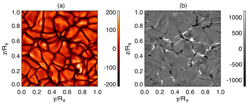
Figure 1: Contours of (a) vertical velocity $v_{x}$ in the unit of $\mathrm{m\ s^{-1}}$ and (b) vertical magnetic field $B_{x}$ in the unit of $\mathrm{G}$ are shown at $r=0.95R_{\odot}$ for case M256D.

The subscripts 0 and 1 denote that background and time-dependent perturbed values. Except for the geometry, the setting is similar to that presented in Paper I. While a limited horizontal extent of the calculation domain is required in order to increase the resolution, we also intend to avoid boundary effect from the side boundaries. Thus we use a periodic boundary and Cartesian geometry. One disadvantage of this setting is that it leads to the incorrect energy flux in the upper part of the domain. The solar energy flux at the base of the convection zone ($r=0.715R_{\odot}$, where $R_{\odot}$ is the solar radius), is about $1.21\times 10^{11}\ \mathrm{erg\ s^{-1}\ cm^{-2}}$. This is about twice as large as the flux found in the photosphere due to the expansion factor of $r^{2}$. We should keep in mind that the obtained convective velocity will be larger by less than factor of $\sqrt{2}$ in the upper part of the domain. The scaling law of $v^{2-3}\propto F$ is found in some studies even in rapid rotation situation (Christensen 2010; Schrinner et al. 2014; Hotta et al. 2015), which is not far from mixing length theory, which predicts the dependence of $v^{3}\propto F$ (e.g. Stix 2004). The background stratification, $\rho_{0}$, $p_{0}$, and $T_{0}$, is obtained by solving the hydrostatic equation in the adiabatic atmosphere. The gravitational acceleration $g$ and the radiative diffusivity $\kappa_{\mathrm{r}}$ are adopted from the Model S (Christensen-Dalsgaard et al. 1996). The obtained stratification is almost same as the Model S (see Fig. 1 of Paper I). The same form for the surface cooling $\Gamma$ is adopted as in Paper I. The thickness of the cooling layer is two pressure scale heights at the top boundary, which is 18.8 Mm. We use a realistic equation of state, which include the partial ionization effects using OPAL repository (Rogers et al. 1996) is used in eq. (5), the plasma is almost completely ionized in the calculation domain of this study. Thus the equation of state is almost the same as that for an ideal gas. The factor for the RSST is set for keeping the reduced adiabatic speed of sound $\hat{c_{s}}=c_{s}/\xi$ constant as

$$\xi(x)=\xi_{0}\frac{c_{\mathrm{s}}(x)}{c_{\mathrm{s}}(x_{\mathrm{min}})},$$ (6)

where $c_{s}(x)=\sqrt{(\partial p/\partial\rho)_{s}}$ and $x_{\mathrm{min}}$ the original adiabatic speed of sound and the location of the bottom boundary. We use $\xi_{0}=150$ and the reduced speed of sound $\hat{c_{\mathrm{s}}}$ is $1.5\ \mathrm{km\ s^{-1}}$. Considering the validity of the RSST, i.e. $v_{\mathrm{rms}}/{\hat{c_{\mathrm{s}}}}<0.7$, we can properly treat the convection of $v_{\mathrm{rms}}<1.05\ \mathrm{kms^{-1}}$, where $v_{\mathrm{rms}}$ is root mean square (RMS) velocity. In addition to increasing the effective resolution, we also adopt a less diffusive artificial viscosity suggested in Rempel (2014). We note that this modification has a significant effect on resolving the small-scale magnetic field and leads to significantly larger kinematic growth rates, i.e. more efficient small-scale dynamos.

Our calculation domain extends $(0.715R_{\odot},0,0)<(x,y,z)<(0.96R_{\odot},R_{\odot},R_{\odot})$. The periodic boundary condition is adopted for the $y$- and $z$-directions ($x$ is vertical). The symmetric boundary condition is adopted for density and the entropy perturbation at the top and bottom boundaries. Impenetrable and stress-free boundary condition are adopted for the velocity ($v_{x}=\partial v_{y}/\partial x=\partial v_{z}/\partial x=0$). At the top boundary, the horizontal magnetic field is zero ($B_{y}=B_{z}=0$). At the bottom boundary a symmetric boundary condition is adopted for the horizontal magnetic field. Then the vertical magnetic field $B_{x}$ is calculated to satisfy the $\nabla\cdot{\bf B}=0$ constraint at top and bottom boundaries. In the calculation domain the divergence free condition for the magnetic field is maintained with the method suggested by Dedner et al. (2002).

Our investigation is focused on the solar convection zone. Since we investigate the contribution from a small-scale dynamo alone, we do not include rotation. In this setup the stratification and the luminosity are well determined by a solar standard model (Christensen-Dalsgaard et al. 1996). The free parameters in this study are domain extent and resolution (which translates into diffusivities since we use an LES (Large Eddy Simulation) approach). The typical scale of stratified convection is determined by the local pressure scale height, which reaches a value of $\sim$ 60 Mm at the base of the convection zone. Our horizontal extent of 700 Mm is large enough to expect at best a weak influence. The vertical extent of our domain from $0.715$ to $0.96\,R_{\odot}$ was chosen to capture most of the convection zone, but leaves out scales near the top, which are too small to be resolved. Since we focus here on small-scale dynamo simulations it is not sufficient to just resolve the scale of convection, we need to be able to resolve also a significant fraction of the turbulent energy cascade. The effective magnetic and fluid Reynolds numbers are tied to the grid resolution in our study due to the use of an LES approach. Estimating the fluid and magnetic Reynolds numbers is a difficult task (Rempel 2014). We present one simulation with an explicit magnetic diffusivity for which we find a value of $\mathrm{Rm}$ in the range from $300$ to $1200$ (see following paragraph). In our highest resolution LES simulation the small-scale dynamo has an about $100$ times larger growth rate, which indicates a substantially (at least 2 orders of magnitude) larger ”effective” magnetic Reynolds number in those setups. (Note that scaling arguments suggest for the growth rate of a small-scale dynamo $\gamma\sim\sqrt{\mathrm{Rm}}$, which would imply an effective $\mathrm{Rm}$ a factor of $10^{4}$ larger, however, Pietarila Graham et al. (2010); Rempel (2014) found more a $\gamma\sim\mathrm{Rm}$ relationship for the resolutions currently accessible by numerical simulations.)

We carry out four hydrodynamic cases and corresponding four MHD cases. The difference is mainly in the resolution (see Table 1). The characters “H” and “M” denote hydrodynamic and MHD. Cases H256D and M256D include explicit thermal diffusivity, kinetic viscosity and magnetic diffusivity in order to compare the result with previous solar global dynamo calculations. The thermal diffusivity($\kappa$), kinetic viscosity($\nu$) and the magnetic diffusivity($\eta$) are added as:

$$\rho_{0}\frac{\partial{\bf v}}{\partial t} = [...]-\nabla\cdot{\bf D},$$ (7)

$$\frac{\partial{\bf B}}{\partial t} = [...]-\nabla\times(\eta\nabla\times{\bf B}),$$ (8)

$$\rho_{0}T_{0}\frac{\partial s_{1}}{\partial t} = [...]+\nabla\cdot\left(\kappa\rho_{0}T_{0}\nabla s_{1}\right)$$ (9)

$$+2\rho_{0}\nu\left[e_{ij}e_{ij}-\frac{1}{3}(\nabla\cdot{\bf v})^{2}\right]+\frac{\eta}{4\pi}(\nabla\times{\bf B})^{2},$$

where ${\bf D}$ is the viscous stress tensor defined as

$$D_{ij}=-2\rho_{0}\nu\left[e_{ij}-\frac{1}{3}(\nabla\cdot{\bf v})\delta_{ij}\right],$$ (10)

and $e_{ij}$ is the strain rate tensor. The distribution of $\nu$ and $\eta$ are similar to Fan & Fang (2014). At the top boundary, the value is $1\times 10^{12}\ \mathrm{cm^{2}\ s^{-1}}$ and these decrease with depth following a $1/\sqrt{\rho_{0}}$ profile. This setting is common in ASH (Anelastic Spherical Harmonic) calculation (Miesch et al. 2000; Brun et al. 2004). In this study we adopt the same value for the thermal diffusivity as the other values ($\kappa=1\times 10^{12}\ \mathrm{cm^{2}\ s^{-1}}$). We use the definition of the magnetic Reynolds number $\mathrm{Re}=v_{\mathrm{rms}}d_{\mathrm{c}}/\eta$ (e.g. Gastine et al. 2012), where $d_{\mathrm{c}}$ is the thickness of the convection zone. The estimated magnetic Reynolds number is 336 and 1250 at the top and bottom of the calculation domain, respectively. $v_{\mathrm{rms}}$ is obtained from the result. This is the comparable value to the recent high resolution calculations (Brown et al. 2010, 2011; Gastine et al. 2012; Fan & Fang 2014; Jones 2014; Yadav et al. 2014) All calculations started from a hydrodynamic case and were evolved for 100 days. Then, weak random magnetic field ($B_{z}$) with amplitude of 100 G is added to initiate a small-scale dynamo. The imposed magnetic field is uniform in the $z-$direction and random in the $x-y$ plane. The name of cases becomes “M” correspondingly. In the highest resolution case (H2048 and M2048), the grid spacing is smaller than 350 km.

3 Results

3.1 Structure of velocity and magnetic field

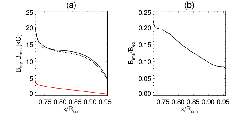
Figure 3: (a) Black lines shows the equipartition magnetic field to the kinetic energy ($B_{\mathrm{eq}}=\sqrt{4\pi\rho_{0}}v_{\mathrm{rms}}$). Solid and dotted lines shows results in MHD (M256D) and hydrodynamic (H256D) cases. Red line shows the RMS magnetic field. (b) The ratio of $B_{\mathrm{rms}}$ to $B_{\mathrm{eq}}$ in case M256D.

We start our discussion with cases H256D and M256D. These mimic the currently available global dynamo calculations. The grid spacing is 2700 km and the explicit diffusivities are included. We note that almost isotoropic grid spacing is used in this paper, i.e, $\Delta x\sim\Delta y=\Delta z$. We calculate case M256D for 2000 days in order to cover its long time scale to the saturated phase. Figs. 1a and b show the contour of vertical velocity $v_{x}$ and vertical magnetic field $B_{x}$ at $r=0.95R_{\odot}$, respectively. As is often seen in global dynamo calculations (e.g. Brun et al. 2004), broad upflows are surrounded by thin downflows. The vertical magnetic field is concentrated in the downflow region. Fig. 2 shows the temporal evolution of magnetic energy averaged over the computational domain in case M256D. The e-folding time scale for magnetic energy during the kinematic phase is 112 days. This is longer than the convective time scale at the base of the convection zone, which is $H_{\rho}/v_{\mathrm{rms}}\sim 10\ \mathrm{day}$, where $H_{\rho}$ and $v_{\mathrm{rms}}$ are the density scale height and the RMS velocity, respectively. We note that when we double the diffusivities, i.e., $\kappa=\nu=\eta=2\times 10^{12}\ \mathrm{cm^{2}\ s^{-1}}$, we do not find an excited small-scale dynamo. Fig. 3a shows the distribution of the equipartition magnetic field strength $B_{\mathrm{eq}}=\sqrt{4\pi\rho_{0}}v_{\mathrm{rms}}$ (black lines) and the RMS magnetic field $B_{\mathrm{rms}}$ (red line). The dotted black line shows the result of the hydrodynamic case (H256D). The RMS magnetic field is about 3000 G and 500 G around the bottom and top boundaries, respectively. The small difference of solid and dotted black lines shows that the influence of the Lorentz feedback on the convection is very small in this case. The dynamo in case M256D maintains $0.08B_{\mathrm{eq}}-0.20B_{\mathrm{eq}}$ magnetic field. The result indicates that the small-scale dynamo in currently available global dynamo calculation is not efficient and that the generated magnetic fields have only a negligible effect on the convective velocity. These findings concern only to the contribution from small-scale field. The large-scale field of a dynamo in rapidly rotating systems can have a significantly effect on the turbulence in some studies (e.g. Christensen et al. 1999; Yadav et al. 2014). In the following investigation we decrease the grid spacing to values of less than 350 km, which currently cannot be reached on the global dynamo calculation.

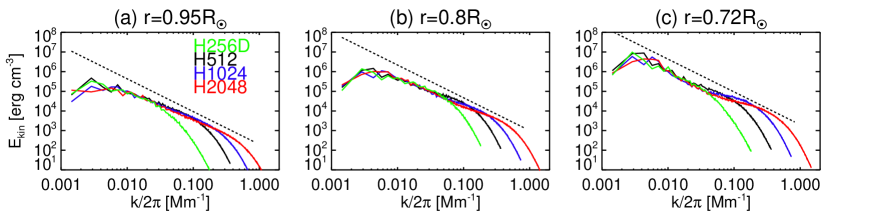
Figure 5: Spectra of kinetic energy at (a) $r=0.95R_{\odot}$, (b) $r=0.8R_{\odot}$, and (c) $r=0.72R_{\odot}$. Green, black, blue, red lines show the results of H256D, H512, H1024, and H2048, respectively. The dotted lines show a Kolmogorov slope of -5/3.

All simulations with higher resolution do not use any explicit diffusivities. The investigation on hydrodynamic cases (H512, H1024, and H2048) is done for the time interval 80-100 days. Fig. 4 shows the distribution of the vertical velocity at $r=0.95R_{\odot}$ (panels a and b) and $r=0.80R_{\odot}$ (panels c and d). Compared with case M256D (Fig. 1a), convection cells are distorted by small-scale turbulence (Fig. 4b). Following the increase of pressure scale height, the typical convection cell size becomes large in the deeper layer. In addition, small-scale turbulence exists much even in the upflow region (Fig. 4d). Figs. 5a, b, and c show the spectra of kinetic energy at $r=0.95R_{\odot}$, $0.8R_{\odot}$, and $0.72R_{\odot}$, respectively for cases H256D, H512, H1024, and H2048. The dotted line indicates a Kolmogorov slope of power-law index $-5/3$. In the upper layer ($r=0.95R_{\odot}$), the spectra of kinetic energy obey the power-low distribution with the index of -5/3 in cases without explicit diffusivities. In the deeper region, especially in $r=0.72R_{\odot}$, there is a depression around $k/2\pi=2\times 10^{-1}\ \mathrm{Mm^{-1}}$ which is largest in case H2048 (red line in Fig. 5c).

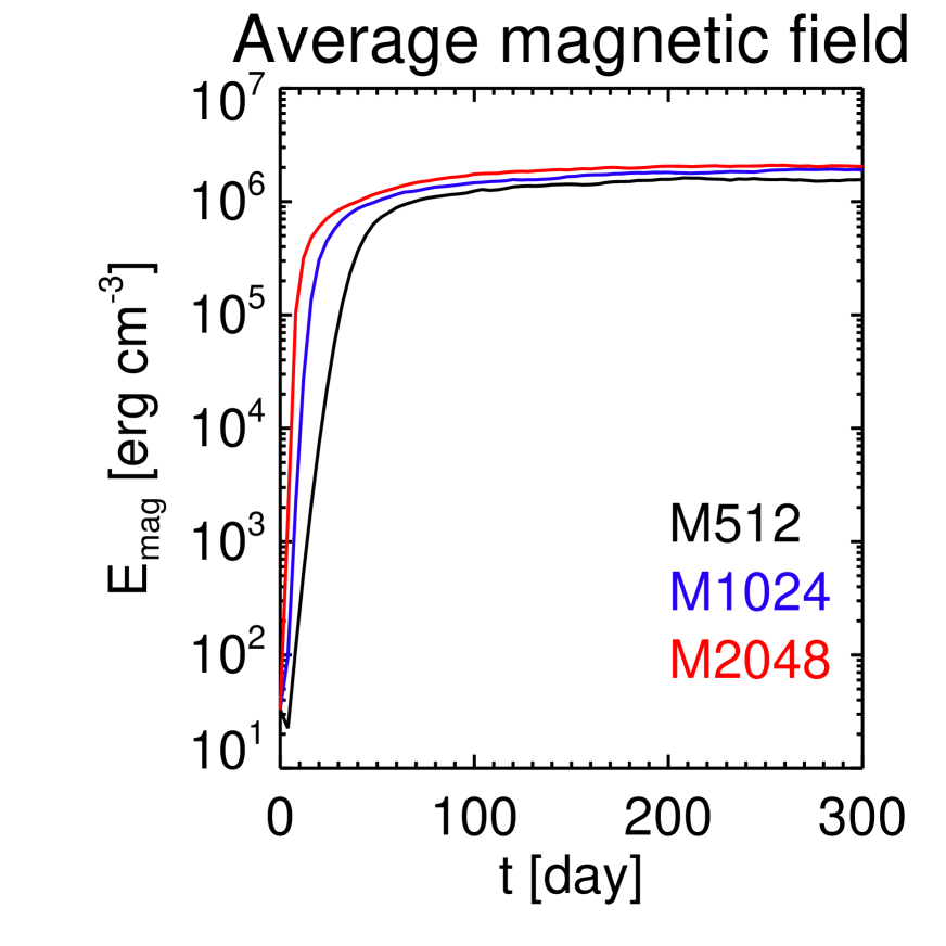
Figure 6: Temporal evolution of magnetic energy. The black, blue, and red lines show the results in cases M512, M1024, and M2048.

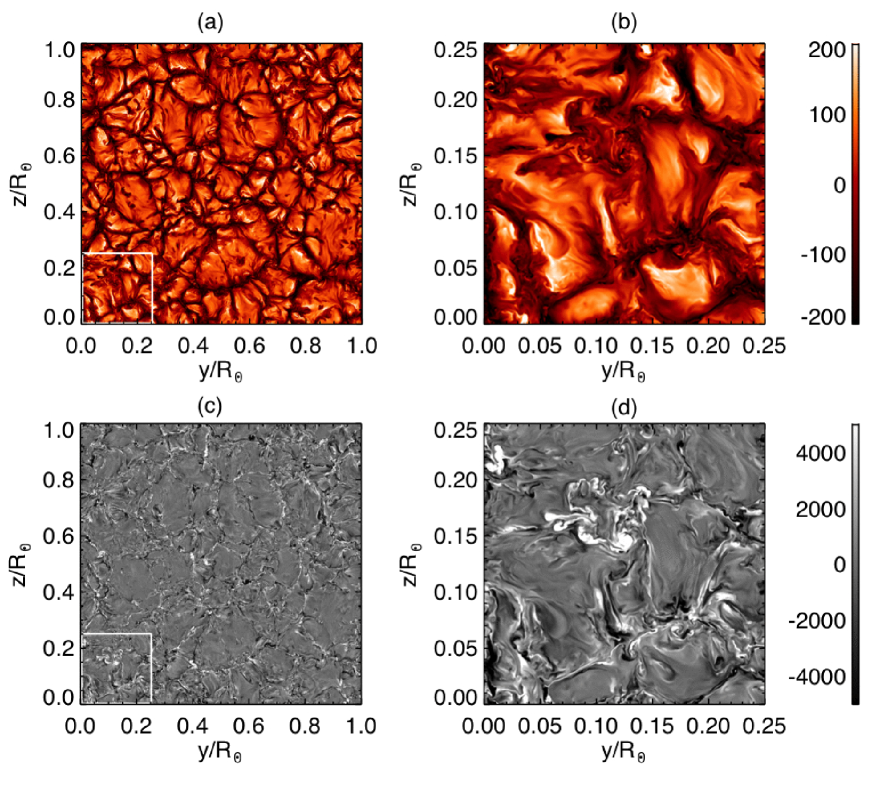
Figure 7: Contour of vertical velocity $v_{x}$ (panels a and b) in the unit of $\mathrm{m\ s^{-1}}$ and vertical magnetic field (panels c and d) in the unit of G are shown at $r=0.95R_{\odot}$ for case M2048. Panels b and d are the zoom-in figure for the panels a and c, respectively.

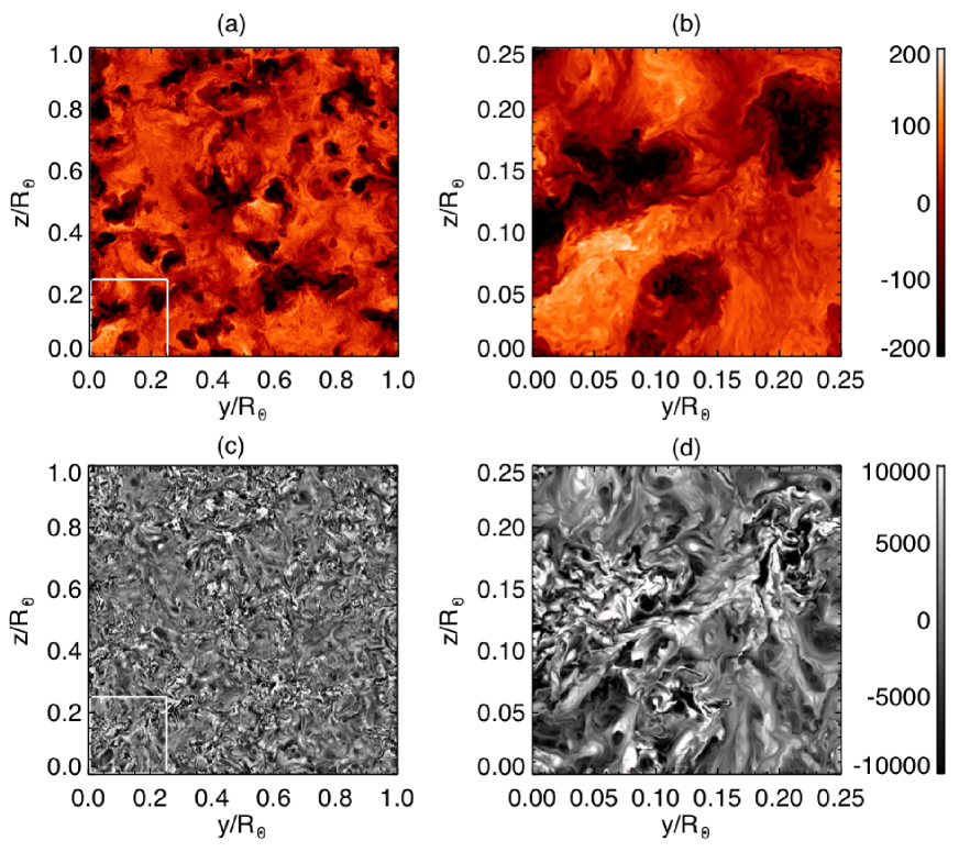
Figure 8: The same format as Fig. 7 at $r=0.8R_{\odot}$.

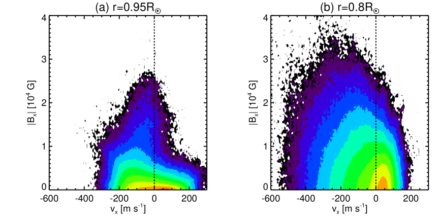
Figure 9: Joint PDFs of vertical velocity ($v_{x}$) in the unit of $\mathrm{m\ s^{-1}}$ and vertical magnetic field ($B_{x}$) in the unit of G in case M2048 at (a) $r=0.95R_{\odot}$ and (b) $r=0.8R_{\odot}$.

Although we calculate the cases M512, and M1024 for 900 days, no significant change can be seen after 300 days. We calculate case M2048 for 300 days and compare the results at the time of 280-300 days. Fig. 6 shows the temporal evolution of magnetic energy averaged over the whole calculation domain. As stated in Rempel (2014), the e-folding time scale for the growth rate of magnetic energy significantly depends on the resolution. The time scales are 3.24, 1.97, and 0.99 days at case M512, M1024, and M2048, respectively. In addition, the saturated magnetic energy is one order of magnitude higher than that in case M256D. The magnetic energy in cases M1024 and M2048 converges around $t=300\ \mathrm{days}$. Figs. 7 and 8 show the distribution of vertical velocity $v_{x}$ and vertical magnetic field $B_{x}$ at $r=0.95R_{\odot}$ and $r=0.8R_{\odot}$, respectively. Compared with the hydrodynamic case (H2048: Fig. 4), the appearance of the convective flow is smoother. The small-scale turbulence in upflow regions is strongly suppressed (see Figs. 4d and 8b). In the upper layer, the location of small-scale features in $v_{x}$ have rough coincidence with the location of strong vertical magnetic field $B_{x}$. Small-scale magnetic field with mixed polarity is preferentially found in downflow regions. In deeper layers, the coincidence between downflow and strong magnetic field is less pronounced. The magnetic field is distributed rather uniformly. Joint PDFs for vertical velocity ($v_{x}$) and vertical magnetic field ($B_{x}$) also show this feature in Fig. 9. While the distribution of magnetic field smoothly connects between up- and downflow region in the deeper layer (panel b), a steep transition is seen near the upper boundary (panel a). We note that the ratio of the RMS values of vertical magnetic field in upflow to that in downflow ($\sim 0.5$) is not different between these layers.

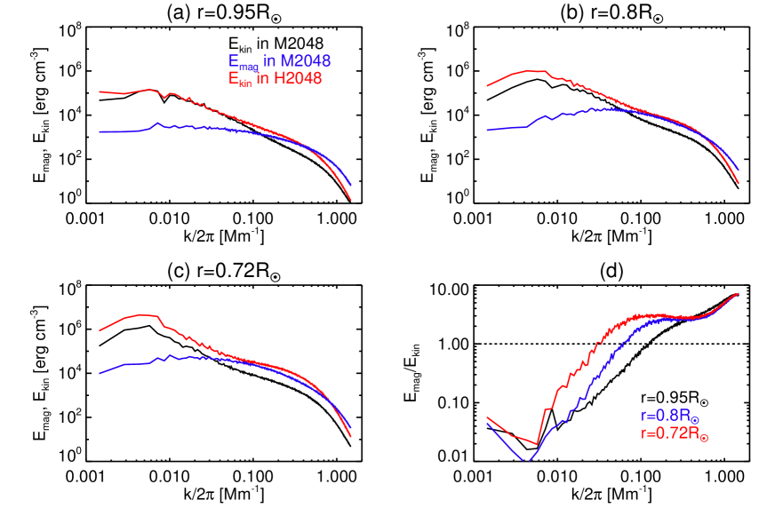
Figure 10: Spectra in cases H2048 and M2048. Panels a, b, and c denote the result at $r=0.95R_{\odot}$, $0.8R$, and $0.72R_{\odot}$. The black and blue lines show kinetic energy, and magnetic energy in case M2048. The red line shows the kinetic energy in case H2048. Panel d shows the ratio of $E_{\mathrm{mag}}$ to $E_{\mathrm{kin}}$ at $r=0.95R_{\odot}$ (black), $0.8R_{\odot}$ (blue), and $0.72R_{\odot}$ (red).

This finding is confirmed with the spectra of magnetic energy $E_{\mathrm{mag}}$ and kinetic energy $E_{\mathrm{kin}}$ in Fig. 10. The black and blue lines show $E_{\mathrm{kin}}$ and $E_{\mathrm{mag}}$ in case M2048. The red lines show $E_{\mathrm{kin}}$ in case H2048. Panels a, b, and c show the results at $r=0.95R_{\odot}$, $0.8R_{\odot}$, and $0.72R_{\odot}$, respectively. Fig. 10d shows the ratio of $E_{\mathrm{mag}}$ to $E_{\mathrm{kin}}$. The black, blue, and red lines show the result at $r=0.95R_{\odot}$, $0.8R_{\odot}$, and $0.72R_{\odot}$, respectively. In every layer, super-equipartition magnetic field is found at small scales. There is depth dependence of the scale where the magnetic energy exceeds the kinetic energy. The scales are 8.1, 15, and 31 Mm for $r=0.95R_{\odot}$, $0.8R_{\odot}$, and $0.72R_{\odot}$, respectively. In Paper I, it is argued that there are two factors that influence the dependence of dynamo efficiency on the depth. One is the negative Poynting flux in the convection zone. In the upper convection zone, magnetic energy is rapidly transport downward and accumulates in the lower convection zone. This makes small-scale dynamo action more challenging near the top and less challenging near the bottom of the domain. The other factor is the dependence of the intrinsic spatial scale of the convection flow on the depth, i.e., the convection in deeper layer has larger spatial scale. For a fixed grid spacing convective structures are better resolved near the bottom of the domain. The super-equipartition magnetic energy is 6 times larger than kinetic energy in the diffusion scale ($k/2\pi>0.5\ \mathrm{Mm^{-1}}$). This likely indicates a numerical magnetic Prandtl number larger than unity in our calculation. In upper layer ($r=0.95R_{\odot}$: Fig. 10a), small-scale kinetic energy is selectively suppressed by magnetic field and the larger scale kinetic energy remains. On the other hand, all the scales are suppressed in the deeper layer at $r=0.72R_{\odot}$ (Fig. 10c).

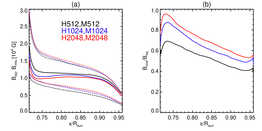
Figure 11: The relation between equipartition magnetic field $B_{\mathrm{eq}}$ and RMS magnetic field $B_{\mathrm{rms}}$. (a) The solid and dash-dotted lines show $B_{\mathrm{eq}}$ and $B_{\mathrm{rms}}$, respectively for the cases M512 (black), M1024 (blue), and M2048 (red). The dotted black, blue, and red lines show $B_{\mathrm{eq}}$ in cases H512, H1024, and H2048, respectively. (b) The ratio of $B_{\mathrm{rms}}$ to $B_{\mathrm{eq}}$ in cases M512, M1024, and M2048.

Fig. 11a shows $B_{\mathrm{eq}}$ and $B_{\mathrm{rms}}$. The solid and dash-dotted lines show $B_{\mathrm{eq}}$ and $B_{\mathrm{rms}}$ in case M512 (black), M1024 (blue), and M2048 (red), respectively. The dotted lines show $B_{\mathrm{eq}}$ in hydrodynamic cases H512 (black), H1024 (blue), and H2048 (red). Although around the base of the convection zone, the strength of the magnetic field between cases M1024 and M2048 converges, the reduction of $B_{\mathrm{eq}}$ is larger in M2048. The higher resolution simulation has more kinetic energy on small scales (recall the depression in Fig. 5c). Since the Lorentz feedback has a larger effect at smaller scales, the reduction of $B_{\mathrm{eq}}$ is larger in case M2048. Fig. 11b shows the ratio of $B_{\mathrm{rms}}$ to $B_{\mathrm{eq}}$ in cases M512, M1024, and M2048. At the base of the convection zone, case M2048 achieves 95% of the equipartition field strength.

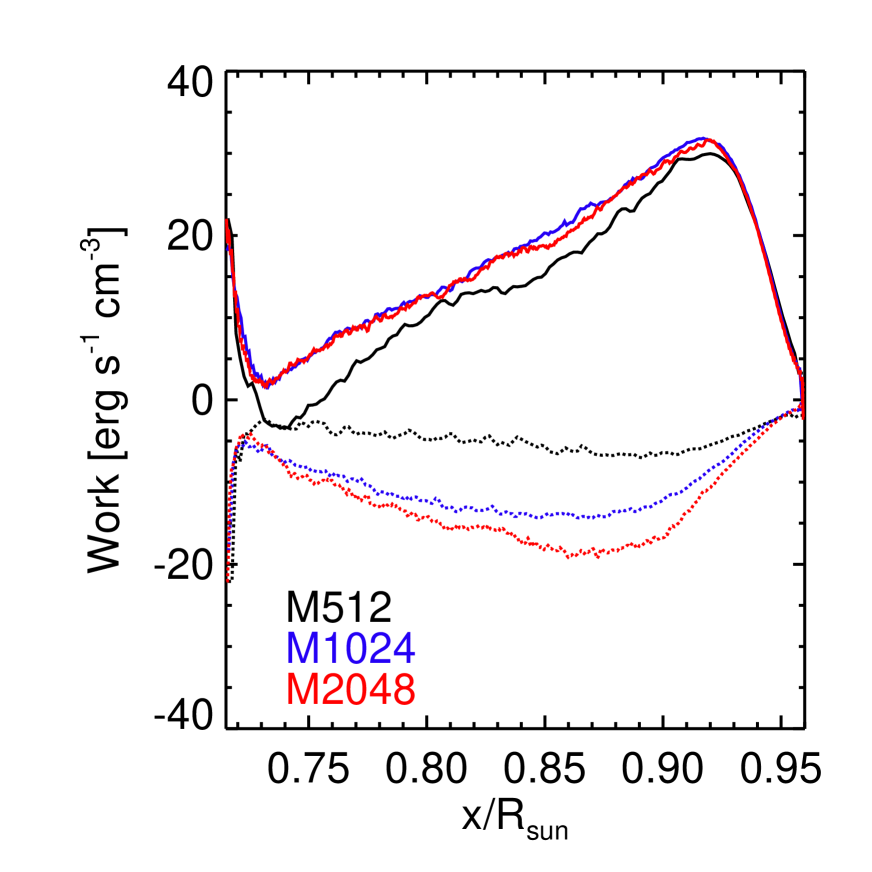
Figure 12: The work densities of pressure/buoyancy ($W_{\mathrm{d}}$: solid line) and the Lorentz force ($W_{\mathrm{l}}$: dotted line) (see eqs. (12) and (11)). The black, blue and red lines show the results of M512, M1024, and M2048, respectively.

Fig. 12 shows the horizontally averaged work densities of pressure/buoyancy ($W_{\mathrm{d}}$) and the Lorentz force ($W_{\mathrm{l}}$) defined as

$$W_{\mathrm{d}} = -\frac{\int{\bf v}\cdot(\nabla p_{1}+\rho_{1}g{\bf e_{x}})dS}{\int dS},$$ (11)

$$W_{\mathrm{l}} = \frac{\int{\bf v}\cdot({\bf j}\times{\bf B})dS}{\int dS},$$ (12)

where $S$ is the horizontal plane. The work by pressure and buoyancy almost converges between M1024 and M2048. The conversion rate from kinetic energy to magnetic energy ($W_{\mathrm{l}}$) is 36%, 61%, and 76% of the pressure/buoyancy work ($W_{\mathrm{d}}$) in the calculation domain in cases M512, M1024, and M2048, respectively. The magnetic Prandtl number is close to unity in this study since we only use numerical diffusivity. Recently Brandenburg (2011, 2014) found that for efficient dynamos with $\mathrm{Rm}\gg 1$ the work by the Lorentz force and consequently the ratio of viscous to resistive energy dissipation is dependent on the magnetic Prandtl number. In particular in the regime $1\ll\mathrm{Rm}\ll\mathrm{Re}$, which is most relevant for solar and stellar convection zones most of the energy dissipation happens through resistivity. This means that the value $W_{\mathrm{l}}/W_{\mathrm{d}}$ increases with lowering the magnetic Prandtl number and should be close to unity (i.e. the small-scale dynamo is maximally efficient). Note that in global dynamo simulations with moderate $\mathrm{Rm}$, where an efficient small-scale dynamo is not present, the value $W_{\mathrm{l}}/W_{\mathrm{d}}$ (mostly due to a large-scale dynamo) can depend on other parameters such as Rossby number (Schrinner 2013).

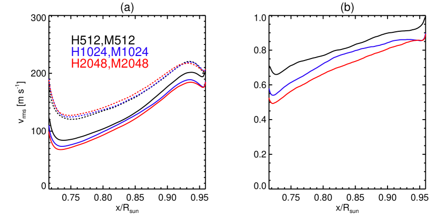
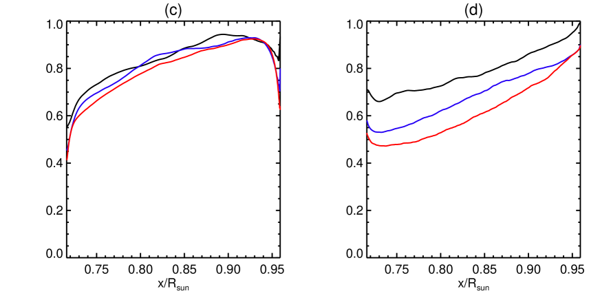
Figure 13: The solid (dotted) black, blue and red lines show the results in cases M512(H512), M1024(H1024), and M2048(H2048), respectively. (a) The distribution of RMS velocities. (b) The ratio of total RMS velocity $v_{\mathrm{RMS}}$ in the MHD cases to hydrodynamic cases, (c) The ratio of vertical RMS velocity $v_{x\mathrm{RMS}}$ in the MHD cases to hydrodynamic cases, and (d) The ratio of horizontal RMS velocity $v_{\mathrm{h\mathrm{RMS}}}$ ($v_{h}=\sqrt{v_{y}^{2}+v_{z}^{2}}$) in MHD cases to hydrodynamic cases.

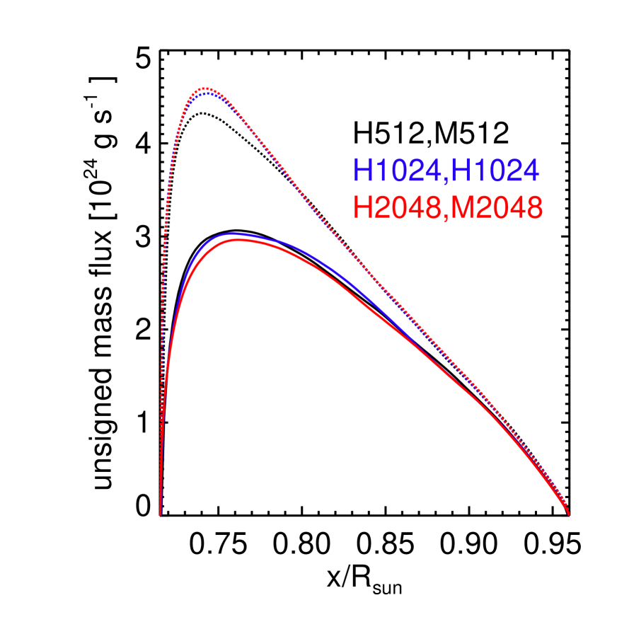
Figure 14: Horizontally integrated unsigned mass flux $\rho_{0}|v_{x}|$. The solid (dotted) black, blue and red lines show the results in cases M512(H512), M1024(H1024), and M2048(H2048), respectively.

Fig. 13 shows the RMS velocity for all cases. In panel a, the solid (dotted), black, blue, and red lines show the results in cases M512 (H512), M1024 (H1024), and M2048 (H2048). Figs. 13b, c, and d show the ratio of RMS velocity in the MHD case to that in the hydrodynamic case. The black, blue and red lines show the result in cases H(M)512, H(M)1024 and H(M)2048. The panels b, c, and d show the RMS velocities including all three components, the x-component, and the horizontal component ($v_{\mathrm{h}}=\sqrt{v_{x}^{2}+v_{y}^{2}}$), respectively. As shown in Fig. 11, Fig. 13 also shows that the reduction of the velocity with magnetic field does not converge with M1024 and M2048. In the highest resolution case M2048, the RMS velocity is reduced to 85% and 50% at the top and bottom boundaries. Figs. 13c and d show that horizontal velocity is more suppressed by magnetic field, which is a key feature for understanding the energy transport in the following discussion. While the suppression of $v_{x}$ is converged, the suppression of $v_{\mathrm{h}}$ shows strong resolution dependence. As shown in the spectra (Fig. 10b and c), the kinetic energy is reduced independently of the spatial scale from the middle to the base of the convection zone. As a result, the unsigned mass flux is also suppressed in the deeper region (Fig. 14). This indicates that the amount of over turning is reduced. It is thought that this is caused by the large-scale magnetic field component, since the reduction does not depend on the resolution significantly.

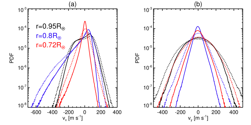
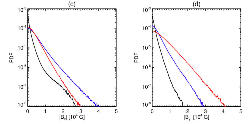
Figure 15: PDFs for (a) the vertical velocity $v_{x}$, (b) a horizontal velocity $v_{y}$, (c) the vertical magnetic field $B_{x}$ and (d) a horizontal magnetic field $B_{y}$. The black, blue and red lines show the result at $r=0.95R_{\odot}$, $0.8R_{\odot}$, and $0.72R_{\odot}$, respectively. The dotted and solid show the result in cases H2048, and M2048.

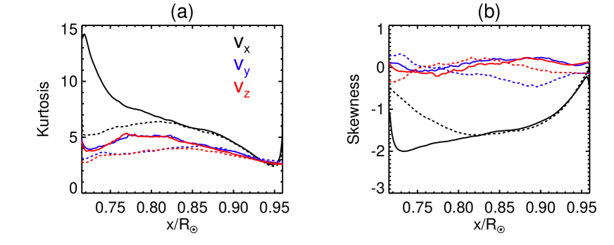
Figure 16: (a) Kurtosis and (b) skewness of the velocities. Black, blue and red lines show $v_{x}$, $v_{y}$, and $v_{z}$, respectively. Dotted and solid lines show the results of H2048 and M2048, respectively.

Figs. 15a, and b show PDFs for $v_{x}$, and $v_{y}$, respectively. The dotted and solid lines show the results in cases H2048 and M2048. The black, blue and red lines show the result at $r=0.95R_{\odot}$, $0.8R_{\odot}$, and $0.72R_{\odot}$, respectively. As shown in Paper I, the vertical velocity has a asymmetric distribution and the distribution of the horizontal velocity is almost Gaussian. Larger velocity values are more strongly reduced at all depths. Fig. 16 shows the kurtosis $\mathcal{K}$ and skewness $\mathcal{S}$, which show intermittency and asymmetry of distribution, respectively. As explained above, the horizontal velocity has almost Gaussian distribution ($\mathcal{K}\sim 3$ and $\mathcal{S}\sim 0$) and vertical velocity ($v_{x}$) has higher intermittency and asymmetry in the hydrodynamic case (H2048: dotted lines). When the magnetic field is included (M2048: solid line), intermittency is increased especially at the bottom part of the convection zone. This indicates that the higher velocity is selectively suppressed by the magnetic field. Figs. 15c and d show PDFs for $B_{x}$, and $B_{y}$, respectively. The PDFs of magnetic field are similar to those in Rempel (2014). Due to the boundary condition at the bottom, the vertical magnetic field at $r=0.8R_{\odot}$ is larger than that in $r=0.72R_{\odot}$. The peak magnetic field strength is around 65 kG near the base of the convection zone. Although we do not generate flux concentrations that are large enough to lead to flux emergence, the achieved magnetic field is sufficiently strong in order to reproduce the active region features (Weber et al. 2011; Hotta et al. 2012a). The vertical field around the top boundary (black line in Fig. 15c) shows an extended tail. Although this is also seen in photospheric simulations, our result is likely strongly influenced by the impenetrable boundary condition at the top.

3.2 Energy transport in high resolution calculations

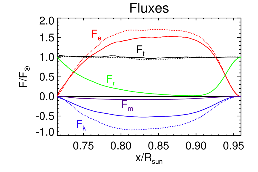
Figure 17: Energy fluxes in cases H2048 and M2048 (dotted and solid lines, respectively). The black, blue, red, light green, and purple lines show the total, kinetic, enthalpy, radiative, and Poynting fluxes, respectively. Black solid line shows the $F=0$ axis for a reference. The solar flux in this study is $F_{\odot}=1.21\times 10^{11}\ \mathrm{erg\ s^{-1}\ cm^{-2}}$.

Fig. 17 shows the horizontally averaged vertical energy fluxes. The definition of the enthalpy flux $F_{\mathrm{e}}$, the kinetic flux $F_{\mathrm{k}}$, the radiative flux $F_{\mathrm{r}}$, the Poynting flux $F_{\mathrm{m}}$, and total flux $F_{\mathrm{t}}$ are shown as

$$F_{\mathrm{e}} = \left(\rho_{0}e_{1}+p_{1}-\frac{p_{0}\rho_{1}}{\rho_{0}}\right)v_{r},$$ (13)

$$F_{\mathrm{k}} = \frac{1}{2}\rho_{0}v^{2}v_{r},$$ (14)

$$F_{\mathrm{r}} = -\kappa_{\mathrm{r}}\rho_{0}c_{p}\frac{dT_{0}}{dr}+\int_{x_{\mathrm{min}}}^{x}\Gamma(x)dx,$$ (15)

$$F_{\mathrm{m}} = \frac{c}{4\pi}(E_{y}B_{z}-E_{z}B_{y}),$$ (16)

$$F_{\mathrm{t}} = F_{\mathrm{e}}+F_{\mathrm{k}}+F_{\mathrm{r}}+F_{\mathrm{m}},$$ (17)

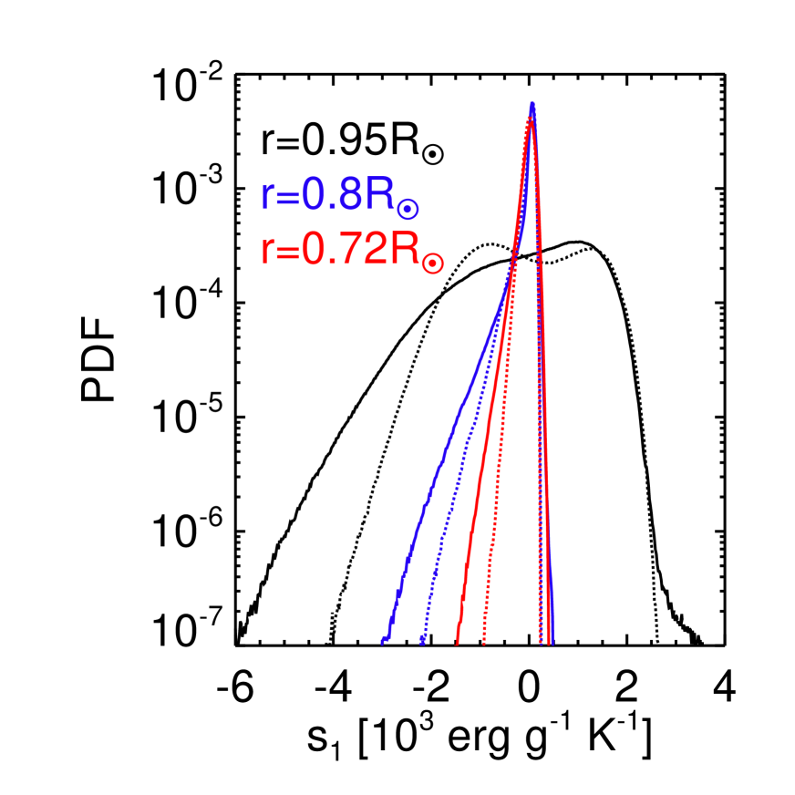
Figure 18: PDFs of the entropy. The black, blue and red lines show the result at $r=0.95R_{\odot}$, $0.8R_{\odot}$, and $0.72R_{\odot}$. The dotted and solid lines show the results in cases H2048 and M2048, respectively.

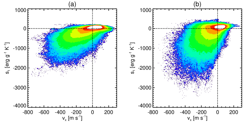
Figure 19: Joint PDFs with the vertical velocity $v_{x}$ and the entropy $s_{1}$ at $r=0.80R_{\odot}$. The panels a and b shows the result in cases H2048 and M2048, respectively.

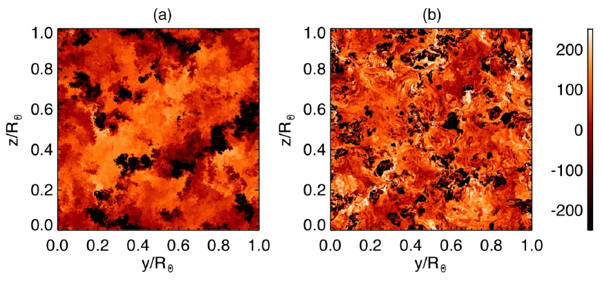
Figure 20: Contour of entropy at $r=0.8R_{\odot}$ in cases (a) H2048 and (b) M2048 in the unit of $\mathrm{erg\ g^{-1}\ K^{-1}}$

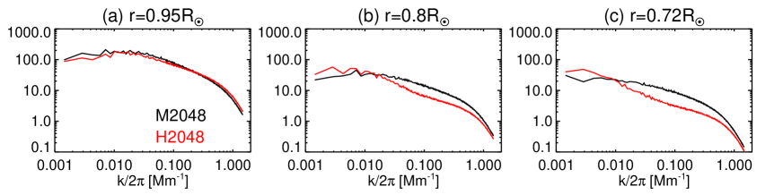
Figure 21: Spectra of entropy at (a) $r=0.95R_{\odot}$, (b) $r=0.8R_{\odot}$, and (c) $r=0.72R_{\odot}$. The red and black lines show the result in cases H2048 and M2048, respectively.

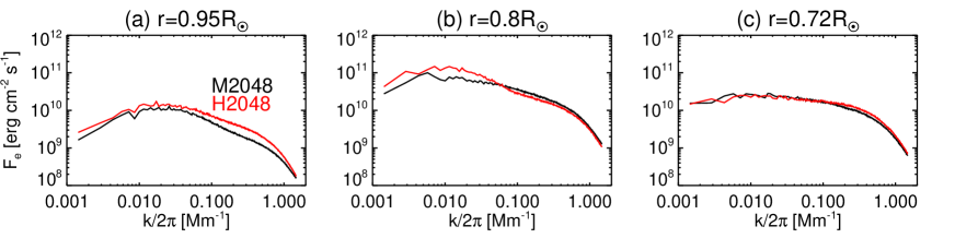
Figure 22: Spectra of enthalpy flux at (a) $r=0.95R_{\odot}$, (b) $r=0.8R_{\odot}$, and (c) $r=0.72R_{\odot}$. The red and black lines show the result in cases H2048 and M2048, respectively.

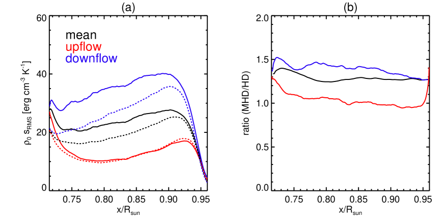
Figure 23: (a) The RMS values of entropy perturbation. Black, red, and blue lines show the mean value, value in upflow and downflow, respectively. Dotted and solid lines show the results in cases H2048 and M2048, respectively. (b) The ratio of the RMS entropy perturbation between the cases H2048 and M2048.

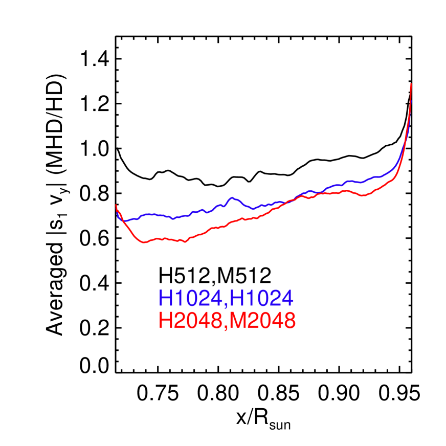
Figure 25: Ratio of horizontally averaged $|s_{1}v_{y}|$ between MHD and HD cases. The black, blue and red lines show the result in cases H(M)512, H(M)1024, and H(M)2048, respectively.

where $e_{1}$ is the internal energy and ${\bf E}=-({\bf v}\times{\bf B})/c$ is the electric field. The artificial surface cooling is included in the radiative flux $F_{\mathrm{r}}$ in order to avoid complexity in the figure. We find a downward directed Poynting flux in our study that reaches 8% of the solar energy flux. This is three times larger than the value found in Paper I. Whereas the reduction in the RMS velocity is large (25% reduction in the middle of the convection zone), the reduction of the enthalpy flux is relatively small (12% at maximum), which implies an increase of the entropy difference between up- and downflows. Fig. 18 shows PDFs of the entropy perturbation. The dotted and solid lines show the results in cases H2048 and M2048, respectively. The black, blue and red lines shows the results at $r=0.95R_{\odot}$, $0.8R_{\odot}$, and $0.72R_{\odot}$, respectively. In every layer, the entropy perturbation, especially in negative part, has larger amplitude in case M2048. Figs. 19a and b show joint PDFs with vertical velocity $v_{x}$ and the entropy perturbation $s_{1}$ in cases H2048 and M2048, respectively. In the MHD case (Fig. 19b), the larger amplitude of the entropy perturbation is achieved in the downflow region. This improves the overall efficiency of the convective energy transport. Figs. 20a and b show the contour of the entropy at $r=0.8R_{\odot}$. Unlike the vertical velocity (Figs. 4a and 8a), the presence of small-scale magnetic field leads to smaller features in the entropy perturbation. In addition the area of negative entropy perturbation is reduced by 20% at maximum. The area of negative entropy perturbation is 30% and 23% at the middle of the convection zone in the cases H2048 and M2048, respectively. This is also seen in the spectra of entropy in Fig. 21. In the deeper layer in particular the small-scale entropy perturbation is amplified. As a result, the enthalpy flux in the middle of the convection is shifted to smaller scales (Fig. 22). In other words, strong magnetic field enhances the small-scale energy transport in the middle of the convection zone. Fig. 23 shows the RMS values of the entropy in cases H2048 and M2048. In the downflow region (blue lines), the amplification of the entropy perturbation is more pronounced. The effect of the magnetic field in upflow region (red lines) is mostly seen around the base of the convection zone. Fig. 24 shows the kurtosis and skewness of the entropy in cases H2048 and M2048. The intermittency and asymmetry of the entropy are increased by the magnetic field. Figs. 13c and d show that the horizontal velocity is more suppressed by the magnetic field than the vertical velocity. In addition, Fig. 25 shows the ratio of horizontally averaged $|s_{1}v_{y}|$ between MHD and HD cases. This is a measure of the reduced horizontal mixing of internal energy between up- and downflows. We find a significant reduction of the horizontal energy mixing with the presence of strong magnetic field. This results in an increased and more efficient energy transport, i.e. the enthalpy flux is not suppressed significantly, despite the reduction of overturning mass.

4 Summary

We presented a series of high resolution MHD simulations in the solar convection zone and studied small-scale dynamo action through the convection zone. For grid spacings smaller than 350 km, the RMS magnetic field around the base of the convection zone reaches 95% of the equipartition field strength. Even around the top boundary 55% of equipartition magnetic field is maintained. These values are consistent with those required in Rempel (2014) to explain the observed field strength of the quiet Sun. We find a significant Lorentz force feedback, the convective RMS velocity is reduced to 50% and 85% compared to the hydrodynamic reference run at the top and bottom boundaries, respectively.

The efficiency of the small-scale dynamo achieved in this study is larger than that of the large-scale dynamo found in many recent global simulations (i.e. we reach substantially stronger $B_{\mathrm{rms}}$ values in our setup with a small-scale dynamo alone).

The significant suppression of the convective velocity does not lead to a significant decrease of the enthalpy flux. This study shows that the suppression of the velocity reduces the horizontal mixing of the entropy between upflow and downflow regions and causes larger entropy perturbations. This improves the efficiency of the convective energy transport. The reduction of the kinetic energy does not converge especially in the lower convection zone where the convective scale is larger, which implies that Lorentz force feedback on convective flows is potentially larger than presented here. Even in that case the horizontal mixing of the entropy might be further reduced leading to even stronger entropy perturbations between up- and downflows and more efficient convective energy transport. Overall we conclude that the Lorentz force feedback from small-scale magnetic field is likely significant and has to be taken into account for realistic simulations of the solar convection zone, which is currently not possible in global simulations.

Recently Hanasoge et al. (2012) presented rather stringent helioseismic constraints on convective velocities in the solar interior, which suggest that current convection simulations overestimate convective velocities by up to several orders of magnitude. In a completely independent study of solar supergranulation through numerical simulations Lord et al. (2014) found that high resolution simulations of the solar photosphere are consistent with observational constraints in the uppermost 10 Mm of the convection zone, but overestimate convective velocities by a factor of a few in more than 10 Mm depth. The work presented here indicates that ubiquitous small-scale magnetic field throughout the solar convection zone might contribute to some degree to resolving the issue, however, the reduction of convective velocities we find is still insufficient. Not completely unrelated to this is likely also the difficulty global convection simulations have in reproducing a solar-like differential rotation in setups that transport a full solar luminosity. The work by Gastine et al. (2014); Käpylä et al. (2014) suggests that a fast rotating equator requires a lower Rossby number, i.e. lower convection velocities throughout the convection zone. Recently Fan & Fang (2014) showed that also Maxwell-stresses from a dynamo generated magnetic field can significantly alter the sign and shape of differential rotation. To which degree this is due to large-scale or small-scale magnetic field components remains at this point an open issue and requires numerical simulations of efficient small-scale dynamos in a global setup with rotation, which is work in progress.

Table 1: Number of grid points and diffusivities in each case.

Case	$N_{x}\times N_{y}\times N_{z}$	$\kappa$, $\nu$, $\eta$ $[\mathrm{cm^{2}\ s^{-1}}]$
H256D, M256D	$72\times 256\times 256$	$1\times 10^{12}$
H512, M512	$144\times 512\times 512$	-
H1024, M1024	$288\times 1024\times 1024$	-
H2048, M2048	$576\times 2048\times 2048$	-

Figure 2: Temporal evolution of magnetic energy averaged over the whole calculation domain in case M256D.

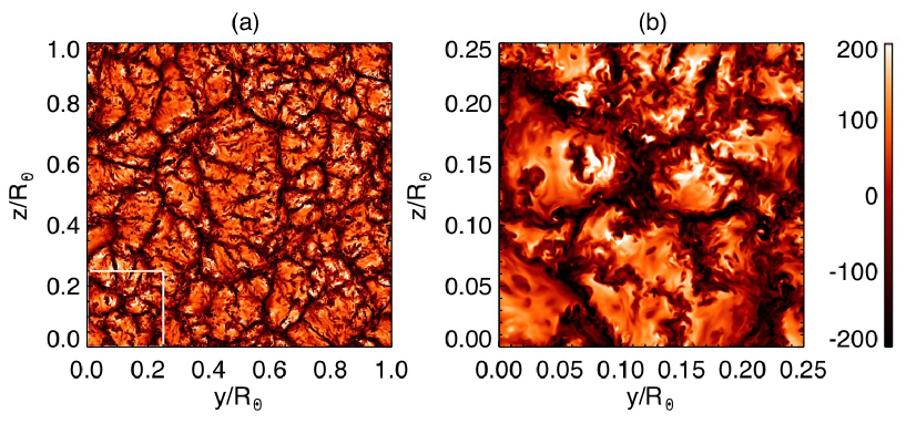
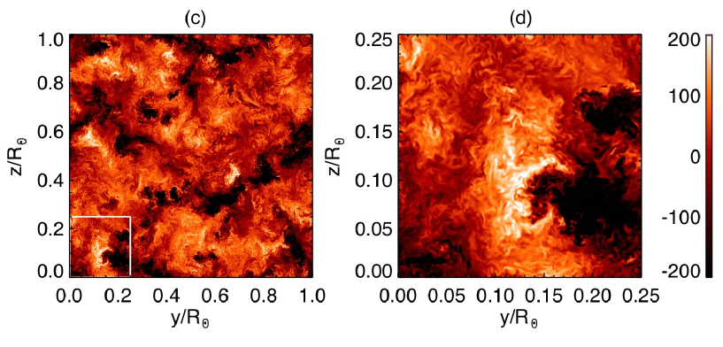
Figure 4: The distribution of vertical velocity $v_{x}$ in case H2048 at $r=0.95R_{\odot}$ (panels a and b) and $r=0.8R_{\odot}$ (panels c and d) in the unit of $\mathrm{m\ s^{-1}}$. Panels b and d show the zoom in image of panels a and c, respectively. The white rectangles indicate the region for panels b and d.

Figure 24: (a) Kurtosis and (b) Skewness of the entropy. Dotted and solid lines show the result in cases H2048 and M2048, respectively.

References

- Augustson et al. (2013) Augustson, K., Brun, A. S., Miesch, M. S., & Toomre, J. 2013, ArXiv e-prints
- Batchelor (1950) Batchelor, G. K. 1950, Royal Society of London Proceedings Series A, 201, 405
- Brandenburg (2011) Brandenburg, A. 2011, Astronomische Nachrichten, 332, 51
- Brandenburg (2014) —. 2014, ApJ, 791, 12
- Brandenburg et al. (1996) Brandenburg, A., Jennings, R. L., Nordlund, Å., Rieutord, M., Stein, R. F., & Tuominen, I. 1996, Journal of Fluid Mechanics, 306, 325
- Brandenburg et al. (2012) Brandenburg, A., Sokoloff, D., & Subramanian, K. 2012, Space Sci. Rev., 169, 123
- Brandenburg & Subramanian (2005) Brandenburg, A., & Subramanian, K. 2005, Phys. Rep., 417, 1
- Brown et al. (2010) Brown, B. P., Browning, M. K., Brun, A. S., Miesch, M. S., & Toomre, J. 2010, ApJ, 711, 424
- Brown et al. (2011) Brown, B. P., Miesch, M. S., Browning, M. K., Brun, A. S., & Toomre, J. 2011, ApJ, 731, 69
- Brun et al. (2004) Brun, A. S., Miesch, M. S., & Toomre, J. 2004, ApJ, 614, 1073
- Brun & Toomre (2002) Brun, A. S., & Toomre, J. 2002, ApJ, 570, 865
- Busse & Simitev (2011) Busse, F., & Simitev, R. 2011, Geophysical and Astrophysical Fluid Dynamics, 105, 234
- Cattaneo (1999) Cattaneo, F. 1999, ApJ, 515, L39
- Charbonneau (2005) Charbonneau, P. 2005, Living Reviews in Solar Physics, 2, 2
- Christensen et al. (1999) Christensen, U., Olson, P., & Glatzmaier, G. A. 1999, Geophysical Journal International, 138, 393
- Christensen (2010) Christensen, U. R. 2010, Space Sci. Rev., 152, 565
- Christensen-Dalsgaard et al. (1996) Christensen-Dalsgaard, J., et al. 1996, Science, 272, 1286
- Dedner et al. (2002) Dedner, A., Kemm, F., Kröner, D., Munz, C.-D., Schnitzer, T., & Wesenberg, M. 2002, Journal of Computational Physics, 175, 645
- Fan & Fang (2014) Fan, Y., & Fang, F. 2014, ApJ, 789, 35
- Gastine et al. (2012) Gastine, T., Duarte, L., & Wicht, J. 2012, A&A, 546, A19
- Gastine et al. (2014) Gastine, T., Yadav, R. K., Morin, J., Reiners, A., & Wicht, J. 2014, MNRAS, 438, L76
- Ghizaru et al. (2010) Ghizaru, M., Charbonneau, P., & Smolarkiewicz, P. K. 2010, ApJ, 715, L133
- Hanasoge et al. (2012) Hanasoge, S. M., Duvall, T. L., & Sreenivasan, K. R. 2012, Proceedings of the National Academy of Science, 109, 11928
- Haugen et al. (2004) Haugen, N. E., Brandenburg, A., & Dobler, W. 2004, Phys. Rev. E, 70, 016308
- Hawley et al. (1996) Hawley, J. F., Gammie, C. F., & Balbus, S. A. 1996, ApJ, 464, 690
- Hotta et al. (2012a) Hotta, H., Rempel, M., & Yokoyama, T. 2012a, ApJ, 759, L24
- Hotta et al. (2014) —. 2014, ApJ, 786, 24
- Hotta et al. (2015) —. 2015, ApJ, 798, 51
- Hotta et al. (2012b) Hotta, H., Rempel, M., Yokoyama, T., Iida, Y., & Fan, Y. 2012b, A&A, 539, A30
- Iskakov et al. (2007) Iskakov, A. B., Schekochihin, A. A., Cowley, S. C., McWilliams, J. C., & Proctor, M. R. E. 2007, Physical Review Letters, 98, 208501
- Jones (2014) Jones, C. A. 2014, Icarus, 241, 148
- Käpylä et al. (2014) Käpylä, P. J., Käpylä, M. J., & Brandenburg, A. 2014, A&A, 570, A43
- Krause & Rädler (1980) Krause, F., & Rädler, K. 1980, Mean-field magnetohydrodynamics and dynamo theory, ed. Goodman, L. J. & Love, R. N.
- Lord et al. (2014) Lord, J. W., Cameron, R. H., Rast, M. P., Rempel, M., & Roudier, T. 2014, ApJ, 793, 24
- Meneguzzi et al. (1981) Meneguzzi, M., Frisch, U., & Pouquet, A. 1981, Physical Review Letters, 47, 1060
- Miesch (2005) Miesch, M. S. 2005, Living Reviews in Solar Physics, 2, 1
- Miesch et al. (2000) Miesch, M. S., Elliott, J. R., Toomre, J., Clune, T. L., Glatzmaier, G. A., & Gilman, P. A. 2000, ApJ, 532, 593
- Ossendrijver (2003) Ossendrijver, M. 2003, A&A Rev., 11, 287
- Parker (1955) Parker, E. N. 1955, ApJ, 122, 293
- Pietarila Graham et al. (2010) Pietarila Graham, J., Cameron, R., & Schüssler, M. 2010, ApJ, 714, 1606
- Rempel (2014) Rempel, M. 2014, ApJ, 789, 132
- Rogers et al. (1996) Rogers, F. J., Swenson, F. J., & Iglesias, C. A. 1996, ApJ, 456, 902
- Schekochihin et al. (2004) Schekochihin, A. A., Cowley, S. C., Maron, J. L., & McWilliams, J. C. 2004, Physical Review Letters, 92, 054502
- Schekochihin et al. (2005) Schekochihin, A. A., Haugen, N. E. L., Brandenburg, A., Cowley, S. C., Maron, J. L., & McWilliams, J. C. 2005, ApJ, 625, L115
- Schekochihin et al. (2007) Schekochihin, A. A., Iskakov, A. B., Cowley, S. C., McWilliams, J. C., Proctor, M. R. E., & Yousef, T. A. 2007, New Journal of Physics, 9, 300
- Schrinner (2013) Schrinner, M. 2013, MNRAS, 431, L78
- Schrinner et al. (2014) Schrinner, M., Petitdemange, L., Raynaud, R., & Dormy, E. 2014, A&A, 564, A78
- Steenbeck & Krause (1969a) Steenbeck, M., & Krause, F. 1969a, Astronomische Nachrichten, 291, 49
- Steenbeck & Krause (1969b) —. 1969b, Astronomische Nachrichten, 291, 271
- Stix (2004) Stix, M. 2004, The sun : an introduction, 2nd edn., Astronomy and astrophysics library, (Berlin: Springer), ISBN: 3-540-20741-4
- Vögler & Schüssler (2007) Vögler, A., & Schüssler, M. 2007, A&A, 465, L43
- Weber et al. (2011) Weber, M. A., Fan, Y., & Miesch, M. S. 2011, ApJ, 741, 11
- Yadav et al. (2013) Yadav, R. K., Gastine, T., & Christensen, U. R. 2013, Icarus, 225, 185
- Yadav et al. (2014) Yadav, R. K., Gastine, T., Christensen, U. R., & Reiners, A. 2014, ArXiv e-prints