Magnetization degree at the jet base of M87 derived from the event horizon telescope data: Testing magnetically driven jet paradigm

Abstract

We explore the degree of magnetization at the jet base of M87 by using the observational data of the event horizon telescope (EHT) at 230 GHz obtained by Doeleman et al. By utilizing the method in Kino et al., we derive the energy densities of magnetic fields ($U_{B}$) and electrons and positrons ($U_{\pm}$) in the compact region detected by EHT (EHT-region) with its full-width-half-maximum size $40~{}{\rm\mu as}$. First, we assume that an optically-thick region for synchrotron self absorption (SSA) exists in the EHT-region. Then, we find that the SSA-thick region should not be too large not to overproduce the Poynting power at the EHT-region. The allowed ranges of the angular size and the magnetic field strength of the SSA-thick region are $21~{}{\rm\mu as}\leq\theta_{\rm thick}\leq 26.3~{}{\rm\mu as}$ and $50~{}{\rm G}\leq B_{\rm tot}\leq 124~{}{\rm G}$, respectively. Correspondingly $U_{B}\gg U_{\pm}$ is realized in this case. We further examine the composition of plasma and energy density of protons by utilizing the Faraday rotation measurement ($RM$) at 230 GHz obtained by Kuo et al. Then, we find that $U_{B}\gg U_{\pm}+U_{p}$ still holds in the SSA-thick region. Second, we examine the case when EHT-region is fully SSA-thin. Then we find that $U_{B}\gg U_{\pm}$ still holds unless protons are relativistic. Thus, we conclude that magnetically driven jet scenario in M87 is viable in terms of energetics close to ISCO scale unless the EHT-region is fully SSA-thin and relativistic protons dominated.

1. Introduction

Elucidating the formation mechanism of relativistic jets in active galactic nuclei (AGNs) is one of the longstanding challenges in astrophysics. Although magnetically driven jet and wind models are widely discussed in the literatures (e.g., Okamoto 1974; Blandford & Znajek 1977; Blandford & Payne 1982; Chiueh et al. 1991; Li et al. 1992; Uchida 1997; Okamoto 1999; Koide et al. 2002; Tomimatsu & Takahashi 2003; Vlahakis & Konigl 2003; McKinney and Gammie 2004; Krolik et al. 2005; McKinney 2006; Komissarov et al. 2007; Komissarov et al. 2009; Tchekhovskoy et al. 2011; Toma & Takahara 2013; Nakamura and Asada 2013; McKinney et al. 2013), the actual value of the strength of magnetic field ($B$) at the base of the jet is still an open problem. In order to test magnetic jet paradigm, it is most essential to clarify the energy density of magnetic fields ($U_{B}\equiv B_{\rm tot}^{2}/8\pi$) and that of particles at the upstream end of the jet where $B_{\rm tot}$ is the strength of total magnetic fields.

Recently, short-millimeter radio observations at 1.3 mm (equivalent to the frequency 230 GHz) have been performed against the nearby giant radio galaxy M87. M87 is located at a distance of $D_{\rm L}=16.7~{}{\rm Mpc}$ (Jordan et al. 2005; Blakeslee et al. 2009), hosts one of the most massive super massive black hole $M_{\bullet}=(3-6)\times 10^{9}~{}M_{\odot}$ (e.g., Macchetto et al. 1997; Gebhardt and Thomas 2009; Walsh et al. 2013) and thus M87 is known as the best target for studying the upstream end of the jet (e.g., Junor et al. 1999; Hada et al. 2011). The Schwarzschild radius is $R_{s}\equiv 2GM_{\bullet}/c^{2}\approx 2\times 10^{15}~{}{\rm cm}$ for the central black hole with $M_{\bullet}=6\times 10^{9}~{}M_{\odot}$ where $G$ is the gravitational constant and $c$ is the speed of light. This corresponds to the angular size of $\sim 7~{}\mu as$. Hereafter, we set this mass as the fiducial one. The Event Horizon Telescope (EHT) composed of stations in Hawaii and the western United States has detected a compact region at the base of the M87 jet at 230 GHz with its size $40~{}\mu$as (Doeleman et al. 2012). Furthermore, Kuo et al. (2014) obtained the first constraint on the Faraday rotation measure ($RM$) for M87 using the submillimeter array (SMA) at 230 GHz.

Short milli-meter VLBI observations of EHT at 230 GHz (equivalent to 1.3 mm) is crucially beneficial in order to minimize the blending effect of sub-structures below the spatial resolutions of telescopes. Historically, single dish observations of AGN jets at centi-meter waveband (with arc-minute spatial resolution) revealed that their spectra are flat at cm waveband (Owen et al. 1978). Marscher (1977) suggested the importance of VLBI observations for distinguishing various possible explanations for the observed flatness. Cotton et al. (1980) conducted VLBI observations at cm waveband and found that the flat spectrum results from a blending effect of sub-structures with milli-arcsecond (mas) scale. This was a significant forward step. However, subsequent VLBI observations have revealed that such mas scale components still have sub-structures when observing them at higher spatial resolution (i.e., shorter wavelength). This is a vicious-circle between telescopes’ spatial-resolutions and sizes of sub-structures. In the case of M87, we finally start to overcome this problem since the spatial-resolution of EHT almost reaches one of the fundamental scales, i.e., ISCO (Innermost Stable Circular Orbit) scale (Doeleman et al. 2012). Hence, in this work, we will assume the ISCO radius ($R_{\rm ISCO}$) as the minimum size of the jet nozzle.

Motivated by the significant observational progresses by EHT, we explore the magnetization degree ($U_{\pm}/U_{B}$) in the core of M87 seen at 230 GHz. We note that Doeleman et al. (2012) did not derive $B_{\rm tot}$ and $U_{\pm}/U_{B}$, and we will estimate them at the EHT-region for the first time. In the theoretical point of view, we have developed the methodology for the estimation of $U_{\pm}/U_{B}$ and $B_{\rm tot}$ in Kino et al. (2014) (hereafter K14), and it is also applicable to 230 GHz. In K14, we estimated $U_{\pm}/U_{B}$ and $B_{\rm tot}$ in the radio core at 43 GHz with $\theta_{\rm FWHM}=110~{}{\rm\mu as}$ and $0.7$ Jy. We obtained the tight constraint of field strength ($1~{}{\rm G}\leq B_{\rm tot}\leq 15~{}{\rm G}$), but the resultant energetics are consistent with either the $U_{\pm}$-dominated or $U_{B}$-dominated ($1\times 10^{-5}\leq U_{\pm}/U_{B}\leq 6\times 10^{2}$). The radio core at 230 GHz with $\theta_{\rm FWHM}=40~{}{\rm\mu as}$ directly corresponds to the upstream end of the M87 jet and then it would give tightest constraints for testing the magnetic jet paradigm. The goal of this work is applying the method of K14 to the EHT-detected region and exploring its properties.

Opacity of EHT-region against SSA is critically important. We should emphasize that it is not clear that EHT-region is SSA-thick or not because short-mm VLBI observations are conducted only at 230 GHz and therefore it is not possible to obtain spectral informations at the moment. Intriguingly, Rioja & Dodson (2011) detect the core shift between 43 and 86 GHz (in Figure 5 in their paper), which means that the radio core at 86 GHz contains the SSA-thick region. With the aid of interferometry observations, we can also infer the turnover frequency. The fluxes measured by IRAM at 89 GHz (Despringre et al. 1996) and SMA at 230 GHz (Tan et al. 2008) also seem to indicate that the radio core is SSA-thick above 89 GHz although the data are not obtained simultaneously (see also Abdo et al. 2009). The sub-mm spectrum obtained by ALMA also shows the spectral break above $\sim 100~{}{\rm GHz}$ (Doi et al. 2013). Therefore, we may infer that SSA turnover frequency for the EHT-region is above $\sim 100~{}{\rm GHz}$. As a working hypothesis, we firstly assume that the EHT-region includes the SSA-thick region and apply the method of K14. We will also discuss the fully SSA-thin case in §6.

The layout of this paper is as follows. In §2, we briefly review the method of K14. In §3, we apply the method to the EHT-region. In §4, the resultant $U_{\pm}/U_{B}$ and $B_{\rm tot}$ are presented. In §5, we further discuss constraints on the proton component. In §6, we discuss the fully SSA-thin case. In §7, we summarize the results and give account of important future work to be pursued. In this work, we define the radio spectral index $\alpha$ as $S_{\nu}\propto\nu^{-\alpha}$.

2. Method

Following K14, here we briefly review the method for constraining magnetic field and relativistic electrons in radio cores.

2.1. Basic assumptions

First of all, we show main assumptions in this work.

• We assume that the emission region is spherical with its radius $R$ which is defined as $2R=\theta_{\rm obs}D_{A}$ where $\theta_{\rm obs}$, $D_{A}=D_{L}/(1+z)^{2}$ and $D_{L}$ are the observed angular diameter of the emission region, the angular diameter distance and the luminosity distance, respectively. This is justified by the following observational suggestion. In the EHT observation of M87 in 2012, Akiyama et al. (2015) measures the closure phase of M87 among the three stations (SMA, CARMA, and SMT). The closure phase is the sum of visibility phases on a triangle of three stations (e.g., Thompson et al. 2001; Lu et al. 2012). Akiyama et al. (2015) shows that the measured closure phases are close to zero ($\lesssim\pm 20^{\circ}$) for the structure detected in Doeleman et al. (2012), which is naturally explained by a symmetric emission region and disfavors significantly asymmetric one.

• We do not include the GR effect for simplicity. The full GR ray-tracing and radiative transfer may be essential for reproducing detailed shape of black hole shadows (e.g., Falcke et al. 2000; Takahashi et al 2004; Broderick & Loeb 2009; Nagakura & Takahashi 2010; Dexter et al. 2012; Lu et al. 2014). However, current EHT can only detect flux from a bright region via visibility amplitude and spatial structure can be constrained only by closure-phases (e.g., Doeleman et al. 2009). Although the predicted black hole shadow images in details seem diverse, the size of the bright region is roughly comparable to ISCO scale (e.g., Fish et al. 2013 for review). Therefore, we do not include the GR effect but explore a fairly wide allowed range for the bright region size $\theta_{\rm thick}$, i.e., from $\sim R_{\rm ISCO}$ to $\sim 2R_{\rm ISCO}$ (see sec. 5).

2.2. General consideration

Given the SSA turnover frequency ($\nu_{\rm ssa}$) and the angular diameter size of the emission region at $\nu_{\rm ssa}$, one can uniquely determine $B_{\rm tot}$ and $K_{\pm}$ where $K_{\pm}$ is the normalization factor of relativistic (non-thermal) electrons and positrons (e.g., Kellerman & Poliny-Toth 1969; Burbidge et al. 1974; Jones et al. 1974a, 1974b; Blandford & Rees 1978; Marscher 1987). Recently, K14 points out that the observing frequency is identical to $\nu_{\rm ssa}$ when we can identify the SSA-thick surface at observing frequency.

As a first step, we assume that the EHT-region is a one-zone sphere with isotropic magnetic field ($B_{\rm tot}$) and particle distributions in the present work. Locally, we denote ($B_{\perp,\rm local}=B_{\rm tot}\sin\alpha$) as the magnetic field strength perpendicular to the direction of electron motion (Ginzburg & Syrovatskii 1965, hereafter GS65) where $\alpha$ is the pitch angle between the vectors of electron velocity and the magnetic field (e.g., Rybicki & Lightman 1979). Then, we can obtain pitch-angle averaged $B_{\perp,\rm local}$ defined as $B_{\perp}$ as follows:

$$B_{\rm tot}^{2}=\frac{3}{2}B_{\perp}^{2}$$ (1)

since $B_{\perp}^{2}=(1/4\pi)\int B_{\rm tot}^{2}\sin^{2}\alpha d\Omega=2B_{\rm tot}^{2}/3$. (This is a slightly different definition of $B_{\perp}$ in K14. The corresponding slight changes of numerical factors are summarized in Appendix.) Since we assume isotropic field, hereafter we choose $B_{\perp}$ direction to the line of sight (LOS).

The number density distribution of relativistic electrons and positrons $n_{\pm}(\epsilon_{\pm})$ is defined as (e.g., Eq.3.26 in GS65)

$$n_{\pm}(\epsilon_{\pm})d\epsilon_{\pm} = K_{\pm}\epsilon_{\pm}^{-p}d\epsilon_{\pm}\quad(\epsilon_{\pm,{\rm min}}\leq\epsilon_{\pm}\leq\epsilon_{\pm,{\rm max}}),$$ (2)

where $\epsilon_{\pm}=\gamma_{\pm}m_{e}c^{2}$, $p=2\alpha+1$, $\epsilon_{\pm,{\rm min}}=\gamma_{\pm,{\rm min}}m_{e}c^{2}$, and $\epsilon_{\pm,{\rm max}}=\gamma_{\pm,{\rm max}}m_{e}c^{2}$ are the electron energy, the spectral index, minimum energy, and maximum energy of relativistic (non-thermal) electrons and positrons, respectively. Although electrons and positrons may have different heating/accerelation process in $e^{-}/e^{+}/p$ mixed plasma (e.g., Hoshino and Arons 1991), here we assume that minimum energies of electrons and positrons are same for simplicity. By evaluating the emission at the synchrotron self-absorption frequency, we obtain

$$B_{\perp} = b(p)\left(\frac{\nu_{\rm ssa,obs}}{1~{}{\rm GHz}}\right)^{5}\left(\frac{\theta_{\rm obs}}{1~{}{\rm mas}}\right)^{4}\left(\frac{S_{\nu_{\rm ssa},\rm obs}}{1~{}{\rm Jy}}\right)^{-2}$$ (3)

$$\times \left(\frac{\delta}{1+z}\right),$$

where $b(p)$ is tabulated in Marscher (1983), Hirotani (2005), and K14. The term $K_{\pm}$ is given by

$$K_{\pm} = k(p)\left(\frac{D_{\rm A}}{1~{}{\rm Gpc}}\right)^{-1}\left(\frac{\nu_{\rm ssa,obs}}{1~{}{\rm GHz}}\right)^{-2p-3}\left(\frac{\theta_{\rm obs}}{1~{}{\rm mas}}\right)^{-2p-5}$$ (4)

$$\times \left(\frac{S_{\nu_{\rm ssa},\rm obs}}{1~{}{\rm Jy}}\right)^{p+2}\left(\frac{\delta}{1+z}\right)^{-p-3},$$

where $k(p)$ is tabulated in K14. The cgs units of $K_{\pm}$ and $k(p)$ depend on $p$: erg^p-1cm^-3. It is useful to show the explicit expression of the ratio $U_{\pm}/U_{B}$ as follows:

$$\frac{U_{\pm}}{U_{B}} = \frac{16\pi}{3b^{2}(p)}\frac{k(p)\epsilon_{\pm,\rm min}^{-p+2}}{(p-2)}\left(\frac{D_{\rm A}}{1~{}{\rm Gpc}}\right)^{-1}\left(\frac{\nu_{\rm ssa,obs}}{1~{}{\rm GHz}}\right)^{-2p-13}$$ (5)

$$\times \left(\frac{\theta_{\rm obs}}{1~{}{\rm mas}}\right)^{-2p-13}\left(\frac{S_{\nu_{\rm ssa},\rm obs}}{1~{}{\rm Jy}}\right)^{p+6}\left(\frac{\delta}{1+z}\right)^{-p-5}$$

$$({\rm for}\quad p>2).$$

From this, we find that $\nu_{\rm ssa,obs}$ and $\theta_{\rm obs}$ have the same dependence on $p$. Using this relation, we can estimate $U_{\pm}/U_{B}$ without minimum energy (equipartition $B$ field) assumption. It is clear that the measurement of $\theta_{\rm obs}$ is crucial for determining $U_{\pm}/U_{B}$.

We further impose two general constraint conditions.

1. Time-averaged total power of the jet ($L_{\rm jet}$) estimated by jet dynamics at large-scale should not be exceeded by the one at the jet base

   $$L_{\rm jet} \geq \max\left[L_{\rm poy},L_{\pm}\right],$$

   $$L_{\pm} = \frac{4\pi}{3}\Gamma^{2}\beta R^{2}cU_{\pm},$$

   $$L_{\rm poy} = \frac{4\pi}{3}\Gamma^{2}\beta R^{2}cU_{B},$$ (6)

   where $L_{\pm}$, $L_{\rm poy}$, $\Gamma$, and $\beta c$ are, respectively, electron/positron kinetic power, Poynting power, bulk Lorentz factor, and bulk speed of the jet at the EHT region. Note that $U_{B}$, $U_{\pm}$, $R$ are directly constrained by VLBI observations.

2. The minimum Lorentz factor of relativistic electrons and positrons ($\gamma_{\pm,\rm min}$) should be smaller than the ones radiating the observed synchrotron emission ($\nu_{\rm syn,obs}$), for example 230 GHz. Otherwise, we would not be able to observe synchrotron emission at the corresponding frequency. This is generally given by

   $$\nu_{\rm syn,obs}\geq 1.2\times 10^{6}B_{\perp}\gamma_{\pm,\rm min}^{2}\frac{\delta}{1+z}.$$ (7)

   These relations significantly constrain on the allowed values of $\gamma_{\pm,\rm min}$ and $B_{\rm tot}$.

In the next section, we will add another constraint condition (i.e., minimums size limit).

3. Application to the EHT-region

Here we apply the method to the EHT-region in M87.

3.1. On basic physical quantities

Here we list the basic physical quantities of the M87 jet.

• The total jet power $L_{\rm jet}$ can be estimated by considering jet dynamics at well-studied bright knots (such as knots A, D and HST-1) located at kpc scale (e.g., Bicknell & Begelman 1996; Owen et al. 2000; Stawarz et al. 2006). Based on the literatures on these studies, here we adopt

  $$1\times 10^{44}~{}{\rm erg~{}s^{-1}}\leq L_{\rm jet}\leq 5\times 10^{44}~{}{\rm erg~{}s^{-1}},$$ (8)

  (see also Rieger & Aharonian 2012 for review). We note that Young et al. (2002) indicates $L_{\rm jet}\sim 3\times 10^{42}~{}{\rm erg~{}s^{-1}}$ based on the X-ray bubble structure which is significantly smaller than the aforementioned estimate.　 The smallness of $L_{\rm jet}$ estimated by Young et al. (2002) could be attributed to a combination of intermittency of the jet and an averaging of $L_{\rm jet}$ on a long time scale of X-ray cavity age. In this work, we do not utilize this small $L_{\rm jet}$.

• We would assume that the bulk speed of the jet is in non-relativistic regime at the jet at the EHT region since both theory and observations currently tend to indicate slow and gradual acceleration so that the flow reaches the relativistic speed around $10^{3-4}~{}R_{s}$ (McKinney 2006; Asada & Nakamura 2014; Hada et al. 2014). The brightness temperature of the 230 GHz radio core is below the critical temperature $\sim 10^{11}~{}{\rm K}$ limited by inverse-Compton catastrophe process (Kellermann & Pauliny-Toth 1969). When the 230 GHz emission originates from the SSA-thick plasma, the characteristic electron temperature is comparable to $T_{b}$ (e.g., Loeb & Waxman 2007) and $T_{b}$ at 230 GHz is in relativistic regime. Therefore, we set

  $$\Gamma\beta=c_{\rm sound=}\frac{1}{\sqrt{3}},$$ (9)

  where $c_{\rm sound}$ is the sound speed of relativistic matter. This will be used in Eq. (1) as $\Gamma^{2}\beta=1/\sqrt{3}$.

• Last, we summarize three differences between this work and Doeleman et al. (2012) in terms of the assumptions on basic physical quantities. In this work, we attempt to reduce assumptions and treat the EHT-region in a more general way. (1) In Doeleman et al. (2012), they assume that the EHT-region size is identical to the ISCO size itself which reflects the degree of the black hole spin. In this work, we do not use this assumption. (2) Doeleman et al. (2012) seems to focus on the SSA-thin case. In this work, we will investigate both SSA-thick and SSA-thin cases. (3) Doeleman et al. (2012) seems to assume $\theta_{\rm FWHM}$ as the physical size of the EHT-region. In this work, we take into account a deviation factor between $\theta_{\rm FWHM}$ and its physical size (e.g., Marscher 1983).

3.2. Difficulties for SSA-thick one-zone model

First, we estimate the magnetic field strength in the EHT region by assuming that all of the EHT-region with $\theta_{\rm FWHM}=40~{}{\rm\mu as}$ is fully SSA-thick. The field strength of EHT-region is estimated as

$$B_{\rm tot} = 3.4\times 10^{2}~{}{\rm G}~{}\left(\frac{\nu_{\rm ssa,obs}}{230~{}{\rm GHz}}\right)^{5}$$ (10)

$$\times \left(\frac{\theta_{\rm obs}}{72~{}{\rm\mu as}}\right)^{4}\left(\frac{S_{\nu_{\rm ssa},\rm obs}}{1.0~{}{\rm Jy}}\right)^{-2}\left(\frac{\delta}{1+z}\right).$$

Marscher (1983) pointed out VLBI measured $\theta_{\rm FWHM}$ is connected with true angular size $\theta_{\rm obs}$ by the relation $\theta_{\rm obs}\approx 1.8\theta_{\rm FWHM}$ for partially resolved sources. (see also Krichbaum et al. 2006; Loeb and Waxman 2007). Taking such deviation into account, we examine the case of $72~{}{\rm\mu as}=1.8\times 40~{}{\rm\mu as}$ for the estimate of $B$-field strength.

What happens with this field strength?

3.2.1 Too large Poynting Power

A severe problem arises if $B_{\rm tot}\approx 3\times 10^{2}~{}{\rm G}$ is realized. Since we assume nearly isotropic random field which can be supported by the low linear polarization degree at 230 Ghz (Kuo et al. 2014), the corresponding Poynting power is given by

$$L_{\rm poy} = 1.5\times 10^{47}~{}{\rm erg~{}s^{-1}}$$ (11)

$$\times \left(\frac{B_{\rm tot}}{300~{}{\rm G}}\right)^{2}\left(\frac{2R}{1.8\times 10^{16}~{}{\rm cm}}\right)^{2}.$$

Here we adopt $2R=1.8\times 10^{16}~{}{\rm cm}=1.8\times 40~{}\mu as\times 16.7~{}{\rm Mpc}$. When total power of the jet (i.e., sum of kinetic and Poynting ones) is conserved along the jet at a large-scale, then this is too large compared with the jet’s mean kinetic power inferred from its large-scale dynamics a few$\times 10^{44}~{}{\rm erg~{}s^{-1}}$ (e.g., Rieger & Aharonian 2012 for review) We emphasize that a constraint on $B_{\rm tot}$ by $L_{\rm poy}$ is almost model-independent.

If we allow some kind of fast magnetic reconnection processes (e.g., Kirk & Skjæraasen 2003; Bessho & Bhattacharjee 2007; Takamoto et al. 2012; Bessho & Bhattacharjee 2012) in order to dissipate magnetic fields at the EHT region, then fast and large variabilities would be naturally expected. However, there is no observational support for such variabilities. Therefore, it seems difficult to realize too large $B_{\rm tot}$ at EHT region.

3.2.2 Too fast synchrotron cooling

Once we obtain a typical value of $B_{\rm tot}$, then we can estimate a typical synchrotron cooling timescale. It significantly characterizes observational behavior of the EHT region. The synchrotron cooling timescale is correspondingly

$$t_{\pm,\rm syn}\approx 1\times 10^{-2}~{}{\rm day}\left(\frac{B_{\rm tot}}{300~{}{\rm G}}\right)^{-2}\left(\frac{\gamma_{\pm}}{10}\right)^{-1}.$$ (12)

This is much shorter than day-scale although the flux at 230 GHz measured by the EHT remains constant during subsequent three days (see the Supplementary Material of Doeleman et al. 2012). Then, a difficulty arises due to this short $t_{\pm,\rm syn}$. The 230 GHz radio emitting electrons are in the so-called fast cooling regime (Sari et al. 1998) in which injected electrons instantaneously cool down by synchrotron cooling. Hence, a slight change/fluctuation of $B$ field strength instantaneously (on timescale $t_{\pm,\rm syn}$) is reflected on the synchrotron flux at EHT region. Hence, for realizing the observed constant flux, a constant plasma supply of $B_{\rm tot}$ and $K_{\pm}$ with very small fluctuation is required to avoid rapid variability/decrease of synchrotron flux. On the other hand, when the magnetic fields are not that large, $t_{\pm,\rm syn}$ can become longer than day scale. Then, we can avoid rapid variability/decrease of synchrotron flux without imposing very small fluctuation of $B_{\rm tot}$ and $K_{\pm}$ in the bulk flow. Since some fine-tuning of $B_{\rm tot}$ and $K_{\pm}$ injection may be able to adjust the observed constant flux density at the EHT region, the too-fast-cooling problem may be less severe than the aforementioned problem on too-large-$L_{\rm poy}$. But it is natural to suppose that smaller $B_{\rm tot}$ realizes in the EHT region to avoid fine tuning of injection quantities.

3.3. Two-zone model

3.3.1 Basic idea

The difficulty of too-large-$L_{\rm poy}$ can be resolved if the EHT-regions is composed of SSA-thick and SSA-thin regions and the angular-size of SSA-thick region ($\theta_{\rm thick}$) is more compact than $\theta_{\rm obs}$, i.e.,

$$\theta_{\rm obs}>\theta_{\rm thick}.$$ (13)

We show an illustration of our scenario in Figure 1. In this solution, most of the correlated flux density detected by EHT is attributed to the emission from the SSA-thin region. Since $\nu_{\rm ssa}$ of the SSA-thin region is by definition smaller than 230 GHz, the magnetic field must be significantly smaller because the field strength is proportional to $\nu_{\rm ssa}^{5}$. Because of this reason, we regard the SSA-thick region as the main carrier of the Poynting power.

Here, we assume the ISCO radius for non-rotating black hole ($R_{\rm ISCO}=6GM_{\bullet}/c^{2}=3R_{s}\equiv\theta_{\rm ISCO}D_{L}$) as the minimum size of SSA-thick region. This corresponds to the angular size $21~{}{\rm\mu as}$. Indeed, theoretical works (Broderick & Loeb 2009; Lu et al. 2014) comparing EHT observations and jet models also indicate the model images with short-mm bright region with their size comparable to ISCO. Therefore, we examine the range of SSA-thick region $\theta_{\rm thick}\geq 21~{}{\rm\mu as}$.

3.3.2 Gaussian fitting with two-components

In Figure 2, we estimate the correlated flux density of this SSA-thick region based on the EHT data. The observed flux data plotted as a function of baseline length are adopted from Doeleman et al. (2012). The black solid curve is the best-fit circular gaussian model by Doeleman et al. (2012). The red solid curve is the best-fit model. The red dashed and dot-dashed curves represent the SSA-thick and the SSA-thin components, respectively.

Below, we explain the details of the gaussian fitting. To determine the correlated flux density for the compact SSA-thick region with its lower limit size $\theta_{\rm FWHM}=21~{}{\rm\mu as}/1.8=11.1~{}{\rm\mu as}$, we conduct the two-component (SSA-thick and thin components) gaussian fitting to the EHT-data. First, we obtain the upper limit of the correlated flux density for the SSA-thick component as $S_{\nu}=0.27~{}{\rm Jy}$. Next, we perform the the two-component (SSA-thick and thin components) gaussian fitting by fixing $\theta_{\rm FWHM}=21~{}{\rm\mu as}/1.8=11.1~{}{\rm\mu as}$ and $S_{\nu}=0.27~{}{\rm Jy}$. Then, we obtain the corresponding size and flux of the extended SSA-thin component $S_{\nu}=0.75~{}{\rm Jy}$ and $\theta_{\rm FWHM}=60~{}{\rm\mu as}$.

4. Results

Here, we limit on $B_{\rm tot}$, $\theta_{\rm thick}$, $U_{\pm}/U_{B}$, in the EHT-region without assuming plasma composition. The critical value $\gamma_{\pm,\rm min}$ is derived by the combination of the jet power limit (Eq. 1) and synchrotron emission limit (Eq. (7)). By eliminating $B_{\rm tot}$, we obtain

$$\gamma_{\pm,\rm min} \leq 1.2\times 10^{2}$$

$$\times \left(\frac{2R}{1.8\times 10^{16}~{}{\rm cm}}\right)^{1/2}\left(\frac{L_{\rm jet}}{5\times 10^{44}~{}{\rm erg~{}s^{-1}}}\right)^{-1/4},$$

where $\nu_{\rm ssa}=230~{}{\rm GHz}$ is used. Since $\gamma_{\pm,\rm min}$ has $R$ dependence, larger $R$ allows slightly larger $\gamma_{\pm,\rm min}$.

In Figure 3, we show the value of $\log(U_{\pm}/U_{B})$ in the allowed ranges of $\gamma_{\pm,\rm min}$ and $B_{\rm tot}$ with $L_{\rm jet}=5\times 10^{44}~{}{\rm erg~{}s^{-1}}$ and $p=3.0$. It is essential to note that the maximum value of $B_{\rm tot}$ is determined by the condition $L_{\rm poy}\leq L_{\rm jet}$ while the minimum value of $B_{\rm tot}$ is governed by the condition of $\theta_{\rm thick}\geq R_{\rm ISCO}/D_{\rm L}\approx 21~{}\mu$as. The right side of the allowed region is determined by the $\nu_{\rm syn,obs}$ limit shown in Eq. (7). Note that the maximum value of $\theta_{\rm thick}=26.3~{}\mu{\rm as}$ is smaller than $40~{}\mu{\rm as}$. This suggests that the EHT-region has a more compact SSA-thick component in it. Interestingly, overall SSA-thick region satisfies $U_{B}\gg U_{\pm}$. If protons do not contribute to jet energetics, then this result supports the magnetically driven jet scenario. In Table 1 we show the resultant allowed values. Summing up, we find that (1) the allowed $\theta_{\rm thick}$ satisfies $21~{}{\rm\mu as}\leq\theta_{\rm thick}\leq 26.3~{}{\rm\mu as}$, and that (2) the allowed fields strength is $50~{}{\rm G}\leq B_{\rm tot}\leq 124~{}{\rm G}$.

When we choose a smaller $L_{\rm j}$, the upper limit of $\theta_{\rm thick}$ and $B_{\rm tot}$ becomes smaller according to Eqs. (3) and (1). When $L_{\rm j}=1\times 10^{44}~{}{\rm erg~{}s^{-1}}$, the allowed $B_{\rm tot}$ and $\theta_{\rm thick}$ are $50~{}{\rm G}\leq B_{\rm tot}\leq 65~{}{\rm G}$ and $21~{}{\rm\mu as}\leq\theta_{\rm thick}\leq 22.4~{}{\rm\mu as}$. In this case, the allowed regions of $B_{\rm tot}$ and $\theta_{\rm thick}$ are very narrow.

We add to note a short comment on brightness temperature. The brightness temperature of the SSA-thick region can be estimated as

$$T_{b} = \frac{S_{\nu,\rm obs}c^{2}}{2\pi k\nu_{\rm syn,obs}^{2}(\theta_{\rm thick}/2)^{2}}$$ (15)

$$\approx 2\times 10^{10}~{}K\left(\frac{S_{\nu,\rm obs}}{0.27~{}{\rm Jy}}\right)\left(\frac{\theta_{\rm thick}}{21~{}{\mu\rm as}}\right)^{-2},$$

where $\nu_{\rm syn,obs}=230~{}{\rm GHz}$. This value is comparable with the $T_{b}$ at 86 GHz estimated by Lee (2013).

Last, it is worth to add one thing. According to the equation of state in relativistic temperature regime (e.g., Chandrasekhar 1967; Kato, Fukue & Mineshige 1998), we obtain

$$\gamma_{\pm,\rm ssa}\approx 3\frac{kT_{b}}{m_{e}c^{2}}\approx 10\left(\frac{\theta_{\rm thick}}{21~{}{\rm\mu as}}\right)^{-2},$$ (16)

where we use the fact that $\gamma_{\pm,\rm min}m_{e}c^{2}$ can be identical to the average energy of electrons and positrons since $p$ is steeper than $2$. The obtained $\gamma_{\pm,\rm ssa}$ tends to be smaller than the minimum Lorentz factor obtained by Eq. (4) by a factor of a few. While we may use $\gamma_{\pm,\rm ssa}$ as $\gamma_{\pm,\rm min}$, we conservatively use the condition Eq. (4) taking some uncertainty of numerical factor in Eq. (4) into account.

5. Constraints on proton component

In § 5, we investigate constraint on the energy density of protons ($U_{p}$) by using Faraday $RM$ measured by Kuo et al. (2014). From the measured $RM$, we will constrain the number density of protons ($n_{p}$). Then, we examine $U_{p}$. The degree of proton contribution in energetics has a significant influence over relativistic jet formation (e.g., Begelman, Blandford & Rees 1984; Reynolds et al. 1996).

5.1. Further Assumptions

To discuss the proton contribution, we need to add some further assumptions. Although the observed radio emissions warrant the existence of relativistic $e^{-}/e^{+}$ population, it is not clear about the origin of relativistic $e^{-}/e^{+}$ which radiate radio emissions at 230 GHz. There are several possibilities for its origin. Relativistic protons may play an important role for heating/acceleration of positrons via resonance process with relativistic protons in shocked regions (e.g., Hoshino and Arons 1991), while direct $e^{\pm}$ pair injection (Iwamoto & Takahara 2002; Asano & Takahara 2009), and/or relativistic neutron injection (Toma & Takahara 2012) processes may also work at the jet formation regions. It is beyond the scope of this work to clarify the origin of relativistic $e^{-}/e^{+}$ population and their relation with proton component. In this section, we simply assume the existence of protons and generally define the average energy of these protons as $\epsilon_{p}$.

As mentioned in the Introduction, Kuo et al. (2014) obtained the first constraint on RM for M87 using SMA at 230 GHz. Although it is not clear how much fraction of linearly polarized emission comes from the EHT-region, it is worth to extend the method used in the previous sections by including $RM$ constraint and apply to the present case of 230 GHz core of M87. The degree of LP $\sim 1~{}\%$ at 230 GHz detected by Kuo et al (2014) is significantly smaller than the value when fully-ordered field (i.e., typically $\sim 70~{}\%$ for SSA-thin case and $\sim 16~{}\%$ for SSA-thick case, see Pacholczyk 1970). Hence, the assumption of isotropic $B$-fields in this work looks reasonable to some extent. On the other hand, only ordered magnetic fields aligned to the line of sight ($B_{\rm LOS}$) contribute to the $RM$. Hereafter, we conservatively assume $B_{\rm tot}\geq B_{\rm LOS}$.

5.2. $RM$ limit

Here we introduce a new constraint using $RM$ observation data. This $RM$ is important for estimating the kinetic power of protons ($L_{p}$) because $RM$ can constrain the proton number density. Generally speaking, an observed rotation measure ($RM_{\rm obs}$) consists of two parts, i.e., RM by internal (jet) ($RM_{\rm jet}$) and RM by external (foreground) matter ($RM_{\rm ext}$). Therefore, the $RM_{\rm obs}$ can be decomposed into

$$RM_{\rm obs}=RM_{\rm jet}+RM_{\rm ext}.$$ (17)

Basically, it is difficult to decouple $RM_{\rm jet}$ and $RM_{\rm ext}$ and obtain $RM_{\rm jet}$. However, it may be possible to discuss an upper limit of $|RM_{\rm jet}|$ with some reasonable assumptions. When the observed RM ($RM_{\rm obs}$) is comparable to $RM_{\rm ext}$, then we obtain

$$RM_{\rm obs}\approx RM_{\rm ext},\quad|RM_{\rm jet}|\ll RM_{\rm obs}.$$ (18)

Indeed, foreground Faraday screen in close vicinity of jets seems to well explain observed $RM_{\rm obs}$ for radio-loud AGNs (e.g., Zavala & Taylor 2004) . The explicit form of $RM_{\rm jet}$ the rotation measure for relativistic plasma is given as

$$|RM_{\rm jet}| = \frac{e^{3}}{2\pi m_{e}^{2}c^{4}}\int dlB_{\rm LOS}n_{p}\frac{\log\gamma_{\pm,\rm min}}{2\gamma_{\pm,\rm min}^{2}}$$

$$\leq 5.36\times 10^{3}B_{\rm tot}n_{p}\frac{\log\gamma_{\pm,\rm min}}{2\gamma_{\pm,\rm min}^{2}}\left(\frac{R}{10^{16}~{}{\rm cm}}\right)~{}{\rm rad~{}m^{-2}},$$

where we set $\int dl\approx 2R$ since the region is assumed as uniform. From this, we see that Faraday rotation is strongly suppressed in relativistic plasma (Jones & Odell 1977; Quataert & Gruzinov 2000; Broderick & McKinney 2010). Note that RM only include ionic plasma contribution, and does not include the electron/positron pair plasma. It is because electron and positron have the same mass but have opposite (i.e., minus and plus) charges and then the net Faraday rotation by them is cancelled out. Qualitatively saying, the mixture of $e^{\pm}$ pair plasma (i.e., $\eta<1$) effectively reduce the value of $RM_{\rm jet}$.

Regarding $RM$-limit of M87, Kuo et al. (2014) has measured $|RM_{\rm obs}|\approx(3.4-7.5)\times 10^{5}~{}{\rm rad~{}m^{-2}}$ and they assume $RM_{\rm obs}\approx RM_{\rm ext}$. Following Kuo et al. (2014), we also assume $RM_{\rm obs}\approx RM_{\rm ext}$. Then, the $RM$-limit can be written as

$$|RM_{\rm jet}|\leq 1\times 10^{5}~{}{\rm rad~{}m^{-2}}.$$ (20)

Note that the above constraint only gives the upper limit of $n_{p}$. Therefore, the finite value of $|RM_{\rm jet}|$ does not exclude the plasma composition of pure $e^{\pm}$ plasma.

In sub-section 5.4, we will constrain proton contributions in the case of $B_{\rm tot}\approx B_{\rm LOS}$ in Eq (5.2). At the moment, this is the only case which we can deal with within this simple framework.

5.3. Plasma composition and $e^{\pm}/p$-coupling rate

To further constrain physical properties at the jet base, here we introduce the basic plasma properties and define general notations. The number densities of protons ($n_{p}$) positrons ($n_{+}$), and electrons ($n_{-}$) are, respectively, defined as follows:

$$n_{p} \equiv \eta n_{-},$$

$$n_{+} = (1-\eta)n_{-}\quad(0\leq\eta\leq 1),$$

$$n_{p} = n_{e^{-}p}\approx\frac{\eta}{2-\eta}\frac{1}{p-1}K_{\pm}\gamma_{\pm,\rm min}^{-p+1},$$ (21)

where $\eta$ is a free parameter describing the proton-loading in the jet. Here we use the charge neutrality condition in the jet. It is convenient to define further quantities:

$$n_{\pm} \equiv n_{-}+n_{+}=(2-\eta)n_{-},$$

$$n_{e^{-}p} \equiv \eta n_{-}=n_{p},$$ (22)

where $n_{\pm}$ and $n_{e^{-}p}$ are, the number density of electrons and positrons, and that of proton-associated electrons, respectively. The case of $\eta=0$ corresponds to pure $e^{\pm}$ plasma while $\eta=1$ corresponds to the pure $e^{-}/p$ plasma. Next, it is important to clarify energy balances between electrons and protons. It is useful to introduce the parameter defining the average energy ratio between protons and electrons as $\zeta$ as

$$\epsilon_{\pm}\equiv\zeta\epsilon_{p},\quad(\frac{m_{e}}{m_{p}}\leq\zeta\leq 1),$$ (23)

where $\epsilon_{\pm}$ is the average energy of relativistic $e^{\pm}$. The case $\zeta=1$ can be realized for equipartition between electrons, positrons and protons via effective $e^{\pm}/p$ coupling while $\zeta=m_{e}/m_{p}$ means inefficient $e^{\pm}/p$ coupling for example through randomization of bulk kinetic energy of the jet flow (e.g., Kino et al. 2012 and reference therein). Since we focus on the case of $p>2$ suggested in M87 (Doi et al. 2013), relativistic electrons at minimum Lorentz factors characterize the total energetics. Here, $\epsilon_{\pm}\approx\gamma_{\pm,\rm min}m_{e}c^{2}$ can be estimated as $0.5~{}{\rm MeV}\leq\epsilon_{\pm}\leq 50~{}{\rm MeV}$ together with $1\leq\gamma_{\pm,\rm min}\leq 100$ based on the obtained $\gamma_{\pm,\rm min}$. Then, the case $\zeta=1$ corresponds to that of non-relativistic protons ($0.5~{}{\rm MeV}\leq\epsilon_{p}\leq 50~{}{\rm MeV}$) while the case $\zeta=m_{e}/m_{p}$ coincides with that of relativistic protons ($1~{}{\rm GeV}\leq\epsilon_{p}\leq 100~{}{\rm GeV}$).

In general, $L$ is decomposed to

$$L_{\rm jet} = L_{\pm}+L_{p}+L_{\rm poy},$$

$$L_{\pm} \equiv L_{-}+L_{+},$$ (24)

where $L_{\pm}$, $L_{-}$, $L_{+}$, $L_{p}$, and $L_{\rm poy}$ are, the powers of the sum of electrons and positrons, electrons, positrons, protons, and magnetic fields respectively. For convenience, we define $\eta_{\rm eq}$ for $L_{p}=L_{\pm}$ and it is given by

$$\eta_{\rm eq} \equiv \frac{2\zeta}{1+\zeta},$$

$$L_{p} > L_{\pm}\quad{\rm for}\quad\eta>\eta_{\rm eq},$$

$$L_{p} = L_{\pm}\quad{\rm for}\quad\eta=\eta_{\rm eq},{\rm and}$$

$$L_{p} < L_{\pm}\quad{\rm for}\quad\eta<\eta_{\rm eq}.$$ (25)

Since we set

$$U_{\pm} \approx \epsilon_{\pm}n_{\pm},$$ (26)

$$U_{p} \approx \epsilon_{p}n_{p}=\epsilon_{p}n_{e^{-}p},$$ (27)

$L_{p}/L_{\pm}=U_{p}/U_{\pm}=\eta/[(2-\eta)\zeta]$ holds. Finally, time-averaged total power of the jet ($L_{\rm jet}$) can be generalized as follows:

$$L_{\rm jet} \geq \max\left[L_{\rm poy},\left(1+\frac{\eta}{2-\eta}\frac{1}{\zeta}\right)L_{\pm}\right].$$ (28)

Given the two model parameters $\eta$ and $\zeta$, we obtain $U_{p}$.

5.4. Limits on $B_{\rm tot}$, $\theta_{\rm thick}$, $U_{\pm}/U_{B}$, and $U_{p}/U_{B}$

Here, we give limits on $B_{\rm tot}$, $\theta_{\rm thick}$, $U_{\pm}/U_{B}$, and $U_{p}/U_{B}$ in the EHT-region for $e^{-}/e^{+}/p$ mixed plasma. As for plasma properties, the following four cases with proton loaded plasma can be considered, i.e., relativistic protons with $e^{-}/p$-dominated composition, relativistic protons with $e^{\pm}$-dominated composition, non-relativistic protons with $e^{-}/p$-dominated composition, and non-relativistic protons with $e^{\pm}$-dominated composition.

5.4.1 The case for relativistic protons ($\zeta=m_{e}/m_{p}$)

Here we consider the case for relativistic protons ($\zeta=m_{e}/m_{p})$. In Figure  4, we show a typical example of ”$e^{-}/p$-dominated” case with $\eta=0.99$. In this case, we obtain $\eta_{\rm eq}=1.09\times 10^{-3}$. Since we consider ”$e^{-}/p$-dominated” composition, the upper limit of $RM$ significantly constrains smaller $\gamma_{\pm,\rm min}$ according to Eq. (5.2). In this case, $U_{B}\gg U_{\pm}$ still holds as smaller $\gamma_{\pm,\rm min}$ region is excluded by the $RM$ constraint. In Table 2, we summarize the resultant allowed physical quantities in this case. The maximum value of $B_{\rm tot}$ is determined by the condition $L_{\rm poy}\leq L_{\rm jet}$ while the minimum value of $B_{\rm tot}$ is governed by the condition that $\theta_{\rm thick}\geq R_{\rm ISCO}/D_{\rm L}\approx 21~{}\mu$as. In the limit of inefficient $e^{\pm}/p$ coupling, minimum energy of electrons/positrons are smaller than that of protons by a factor of $m_{e}/m_{p}$ (i.e., $\epsilon_{\pm,\rm min}=(m_{e}/m_{p})\epsilon_{p,\rm min}$). Therefore, $L_{\pm}$ decreases and $L_{p}$ tends to dominate over $L_{\pm}$. The energetics constraint in this case is given by $L_{\rm jet}\geq\max\left[L_{\rm poy},\left(1+\frac{\eta}{2-\eta}\frac{m_{p}}{m_{e}}\right)L_{\pm}\right]$.

In the case of $e^{\pm}$-dominated composition with smaller $\eta$ also leads to the same $B_{\rm tot}$ and $U_{\pm}/U_{\rm B}$. In the same way as shown above, the maximum and minimum values of $B_{\rm tot}$ are determined by the jet power limit and minimum size limit at the EHT-region. However, $U_{p}$ is much smaller than $U_{B}$ simply because of the paucity of the relativistic proton component.

5.4.2 The cases for non-relativistic protons ($\zeta=1$)

Next, let us consider the case of non-relativistic protons ($\zeta=1$). When non-relativistic protons are loaded, the corresponding energetic condition can be given by $L_{\rm jet}\geq\max\left[L_{\rm poy},\left(1+\frac{\eta}{2-\eta}\right)L_{\pm}\right]$. Since the protons are non-relativistic, the effect of proton loading is quite small in terms of energetics. The coefficient resides in a narrow range $1<(1+\eta/(2-\eta))<3/2$. Note that $RM$ strongly depends on $\eta$ while $RM$ is independent of $\zeta$.

The ”$e^{-}/p$-dominated” case results in similar values of $B_{\rm tot}$ and $U_{\pm}/U_{\rm B}$ to those shown in Table 2, because the maximum and minimum values of $B_{\rm tot}$ are also determined by the jet power limit and minimum size limit at the EHT-region. The contribution of protons are only $U_{p}=U_{\pm}/2$. So, it does not give any significant effects on energetics.

Finally, we comment on the ”$e^{\pm}$-dominated” case. The main difference between the ”$e^{-}/p$-dominated” and ”$e^{\pm}$-dominated” cases is $n_{e^{-}p}$. Since the number density of $e^{\pm}$-pairs does not contribute to $RM$, the constraint of $RM$ becomes weaker when $n_{e^{-}p}$ becomes smaller. It leads to wider allowed region for smaller $\gamma_{\pm}$ and smaller $B$ region. Therefore, the maximum value of allowed $U_{\pm}/U_{B}$ for the ”$e^{\pm}$-dominated” case becomes larger than that for ”$e^{-}/p$-dominated” case. However, this only changes the allowed $\gamma_{\pm}$ within a factor of $\sim 10$ and it does not give a large impact on energetics.

6. Fully SSA-thin case

It is worthwhile to examine a case of fully SSA-thin model for EHT-region since the indication of $\nu_{\rm ssa}>100~{}{\rm GHz}$ by interferometry observations does not necessarily mean that $\nu_{\rm ssa}$ is larger than $230~{}{\rm GHz}$. We can safely regard the SSA frequency as $43~{}{\rm GHz}<\nu_{\rm ssa}<230~{}{\rm GHz}$ where the lower limit is warranted by the detection of core-shift at 43 GHz in Hada et al. (2011).

In Figure 5, we show a schematic draw of the synchrotron spectrum when the EHT-region is SSA-thin at 230 GHz (solid line). The upper limit of the flux density at 43 GHz of the 230 GHz core is estimated as $0.09~{}{\rm Jy}=0.7~{}{\rm Jy}\times(40/110)^{2}$ based on the VLBA measurements of the radio core flux and size by Hada et al. (2013). The gray-colored scale shows the typical flux density obtained by SMA and CARMA. Interferometric observation shows some variability at 230 GHz (Akiyama et al. 2015). We define this as $F_{\rm upper}$ and we assume that $F_{\rm upper}$ is the upper limit of the flux density in overall frequency range of $43~{}{\rm GHz}<\nu_{\rm ssa}<230~{}{\rm GHz}$. First, from the EHT data, we can estimate a possible lower limit of $\nu_{\rm ssa}$ as

$$\nu_{\rm ssa} \geq 230~{}{\rm GHz}\times\left(\frac{F_{\rm upper}/2.3~{}{\rm Jy}}{S_{\nu}/1~{}{\rm Jy}}\right)^{-1/\alpha}$$ (29)

$$\sim 160~{}{\rm GHz}~{}({\rm for~{}\alpha=2.5}).$$

Note that, the choice of $\alpha=3.0$ leads to $\nu_{\rm ssa}\sim 170~{}{\rm GHz}$. Second, from the VLBA data, we can estimate a possible upper limit of $\nu_{\rm ssa}$ as

$$\nu_{\rm ssa} \leq 43~{}{\rm GHz}\times\left(\frac{F_{\rm upper}/2.3~{}{\rm Jy}}{S_{\nu}/0.09~{}{\rm Jy}}\right)^{2/5}$$ (30)

$$\sim 160~{}{\rm GHz}.$$

Allowing some flux measurement errors, somehow we can have consistent case around $\nu_{\rm ssa}\sim 160~{}{\rm GHz}$ with $\alpha\sim 2.5$.

Then, let us discuss on physical quantities in this case. From Eq. 5, $U_{\pm}/U_{B}\propto\nu_{\rm ssa}^{-2p-13}$. Therefore, in this case, the ratio would be typically larger by a factor of $(160/230)^{-18}\sim 6.9\times 10^{2}$ (for $p=2.5$) than that for the SSA-thick case. However, this does not change the result of $U_{\pm}\ll U_{\rm B}$ since $U_{\pm}\ll U_{\rm B}<10^{-4}$ in any cases with the SSA-thick core existing. Hence, we can conclude that even for fully SSA-thin EHT-region case, $U_{\pm}\ll U_{\rm B}$ holds in order not to overproduce fluxes between $43~{}{\rm GHz}<\nu_{\rm ssa}<230~{}{\rm GHz}$.

However, a critical difference appears for the comparison between $U_{p}$ and $U_{\rm B}$. In the case of relativistic protons with ”$e^{-}/p$-dominated composition, $U_{p}>U_{B}$ can be realized for a certain range of $\nu_{\rm ssa}$. From the Table 2 we know the values of $U_{p}/U_{B}$ when $\nu_{\rm ssa}=230~{}{\rm GHz}$. By multiplying the factor of $\sim 200-400$ , and the maximum value reaches $U_{p}/U_{B}>1$ at $\nu_{\rm ssa}\sim 160~{}{\rm GHz}$.

7. Summary

We have explored the magnetization degree of the jet base of M87 based on the observational data of the EHT obtained by Doeleman et al. (2012). Following the method in K14, we estimate the energy densities of magnetic fields ($U_{B}$) and electrons and positrons ($U_{\pm}$) in the region detected by EHT (EHT-region) with its FWHM size $40~{}{\rm\mu as}$. Imposing basic energetics of the M87 jet, the constraints from EHT observational data, and the minimum size of the SSA-thick region as the ISCO radius, we find the followings.

• First, we adopt the assumption that the EHT-region contains an SSA-thick region. Then, the co-existence of SSA-thick and SSA-thin regions is required for the EHT-region not to overproduce $L_{\rm poy}$. The angular size of the SSA-thick region is limited as $21~{}{\rm\mu as}\leq\theta_{\rm thick}\leq 25.5~{}{\rm\mu as}$, while that of the SSA-thin region should be $40~{}{\rm\mu as}$ to explain the EHT data. The derived flux density of the SSA-thick region is about 0.27 Jy. The allowed magnetic-fields strength in the SSA-thick region is $58~{}{\rm G}\leq B_{\rm tot}\leq 127~{}{\rm G}$. In terms of energetics, $U_{B}\gg U_{\pm}$ is realized at the overall SSA-thick region. If protons do not dominantly contribute to jet energetics, then this result supports the magnetic-driven jet scenario at the SSA-thick region.

  We further examine the following four cases for electron/positron/proton ($e^{-}/e^{+}/p$) mixed plasma; non-relativistic protons with $e^{-}/p$-dominated composition, non-relativistic protons with $e^{\pm}$-dominated composition, relativistic protons with $e^{-}/p$-dominated composition, and relativistic protons with $e^{\pm}$-dominated composition, together with the assumption that $RM$ detected by SMA (Kuo et al. 2014) gives an upper limit of $RM$ of the EHT-region. Although $RM$ limit can give tighter constraints on allowed $\gamma_{\pm}$, it does not change the results significantly. We find that $U_{B}\gg U_{\pm}$ always holds in any case.

• Second, the case of completely SSA-thin ($\nu_{\rm ssa}<230~{}{\rm GHz}$) EHT-region is also discussed. Although lower $\nu_{\rm ssa}$ can increase the ratio $U_{\pm}/U_{\rm B}$ by a factor of $200-400$ than that for the SSA-thick case, this does not change the result of $U_{\pm}\ll U_{\rm B}$ since $U_{\pm}/U_{\rm B}<10^{-3}$. However, we also find that, in the case of relativistic protons with ”$e^{-}/p$-dominated” composition, $U_{p}>U_{B}$ can be realized around $\nu_{\rm ssa}\sim 160~{}{\rm GHz}$.

Future work and key questions are enumerated below.

• An important future work is to confirm the existence of the SSA-thick region in the EHT-region. If we confirm it, then we can exclude the case of $U_{p}/U_{B}>1$. In the context of confirming the existence of SSA-thick region, we also add to note the effectiveness of inclusions of longer baselines even for a single frequency VLBI observation. In Fig 2, it is clear that the visibility amplitude of the SSA-thin component is much smaller than that of SSA-thick component above $\sim 3G\lambda$ at 1.3mm wavelength. Therefore, inclusions of baselines with $>3G\lambda$ would be effective to distinguish the SSA-thick component. For example, phased ALMA plus SMT with an effective bandwidth of 4 GHz would be effective at $\sim 5G\lambda$ (Fig 6 in Fish et al. 2013). In Figure 2, we show the corresponding baseline-length range (the blue-shaded region).

• Equally important future work is to observe the EHT-region with the spatial resolution of $\sim 1~{}R_{s}$ of M87. Currently, the EHT array with 20-30 $\mu$as resolution at 230 and 345 GHz (e.g., Lu et al. 2014) is not able to reach $\sim 1~{}R_{s}$ of M87. Ground-based short-mm VLBI observations are very sensitive to weather conditions (e.g., Thompson et al. 2001). To confirm our assumption that the minimum $\theta_{\rm thick}D_{L}$ is comparable to $\sim R_{\rm ISCO}$ or even smaller, space VLBI observations would be required in future. In the past missions and existing plan of space VLBI, it was not able to reach the event horizon scale of M87 (e.g., Dodson et al. 2006; Asada et al. 2009; Dodson et al. 2013) since target wavelength were not short enough. Thus, atmospheric-free space (sub-)mm VLBI observation would be indispensable to reach $\sim 1~{}R_{s}$ of M87. The phased ALMA (e.g., Alef et al. 2013, Fish et al. 2013) will play a definitive role for such observations for obtaining visibilities between space and ground telescopes baselines.

  Honma et al. (2014) have recently proposed a new technique of VLBI data-analysis to obtain super-resolution images with radio interferometry using sparse modeling. The usage of the sparse modeling enables us to obtain super-resolution images in which structure finer than the standard beam size can be recognized. A test simulation for imaging of the jet base of M87 is actually demonstrated in Honma et al. (2014) and the technique works well. Therefore, this super-resolution technique will become another important tool for obtaining better resolution images.

• The observational result of Doeleman et al. (2012) does not show flux variability at 230 GHz. However, total epoch-number of EHT observations is too scarce to confirm the absence of flux variability at 230 GHz all of the time. M87 might be in quiescent state during the EHT observations in April 2010 by chance. We also emphasize that the derived field strength is still $\geq 58~{}{\rm G}$ and $t_{\pm,\rm syn}$ still tends to be smaller than day scale. It is also intriguing that the same correlated flux densities in 2009 reported by Doeleman et al. (2012) are observed during another EHT observation performed in April 2012 (Akiyama et al. 2015). This result is quite different from the day scale variability detected in Sagittarius A* by the EHT observations (Fish et al. 2011). To search for a possible flux variability of M87 in more details, continuous monitoring by EHT would be essential.

• Based on GRMHD model, well-ordered poloidal fields are dominant within the Alfven point and toroidal fields become dominant outside of Alfven point while turbulence may not grow-up yet at the jet base (e.g., Spruit 2010 for review). In general, turbulent eddies which most probably generate turbulent fields are not expected before sufficient interactions with surrounding ambient matter (e.g., Mizuta et al. 2010 and reference therein). Therefore, higher LP degree is likely to be expected. Conservatively saying, the reason of low LP degree by Kuo et al. (2014) is most probably because of depolarization within SMA beam. At the moment, we are not able to rule out a possible constitution of RIAF emission which may also lead to low LP degree. If so, then studies of fundamental process for particle accelerations in RIAF (e.g., Hoshino 2013) and the effects particle escape from RIAF (Le & Becker 2004; Toma & Takahara 2012; Kimura et al. 2014) would become more important.

• In terms of the brightness temperature of the 230 GHz radio core of M87 $T_{b}\sim 2\times 10^{10}~{}{\rm K}\left(\frac{S_{\nu}}{1~{}{\rm Jy}}\right)\left(\frac{\theta_{\rm FWHM}}{40~{}{\rm\mu as}}\right)^{-2}$ seems slightly higher than the prediction of hot electron temperature of $\sim 10^{9}~{}{\rm K}$ in RIAF flows (e.g., Manmoto et al. 1997). Hence, the jet emission seems to be preferred to explain EHT-emission in M87 (Dexter et al. (2012), see Ulvestad & Ho (2001) for similar arguments). However, it is not conclusive because geometry near ISCO regions is highly uncertain in observational point of view. The scrutiny of the origin of the 230 GHz emission is still a noteworthy big issue to explore.

• Further　polarimetric observation would be required to examine RM properties in more details. Although we adopt $RM$ values of Kuo at al. (2014), it is found that the observed electric vector position angle (EVPA) trend does not show a sufficiently tight fit to $\lambda^{2}$-law. This behavior may not be due to the consequence of blending of multiple cross-polarized sub-structures with different $RM$ values, but simply rather due to the non-uniformity between the upper and lower side bands of the SMA. A polarimetric observation with ALMA is clearly one of the promising first step to improve this point. Obviously, in the final stage, short-mm (and sub-mm) VLBI polarimetric observations are inevitable to avoid the contamination from the extended region.

• Degree of $e^{\pm}/p$ coupling is a critical factor for the results of the proton power. Theoretically, Hoshino and Arons (1991) found the energy transfer process from protons to positrons via absorptions of high harmonic ion cyclotron waves emitted by the protons. Amato and Arons (2006) indeed performed one-dimensional particle-in-cell (PIC) simulations for $e^{-}/e^{+}/p$-mixed plasma. However, there are several simplifications in PIC simulations such as smaller $m_{p}/m_{e}$ ratio etc. More intensive investigations are awaited to clarify the degree of $e^{\pm}/p$　coupling at the base of the M87 jet.

• We make a brief comment on effects of magnetic field topology and anisotropy of $e^{-}/e^{+}$ in terms of energy distribution. If $e^{-}/e^{+}$ energy distribution in the EHT region is isotropic, then the synchrotron absorption coefficient investigated by GS65 is applicable and differences of field-geometry would not have an impact on field strength estimation. For example, the difference of $B_{\rm tot}$ between the cases of isotropic field (see Eq. (1)) and ordered field ($B_{\perp}=B_{\rm tot}$) which is directed towards LOS is only a factor of $\sqrt{3/2}$.

  However, if the $e^{-}/e^{+}$ energy distribution is highly anisotropic, then the well known synchrotron emissivity and self-absorption coefficient are not applicable. Effects of the $e^{-}/e^{+}$ anisotropy on synchrotron radiation are not well studied and it is beyond the scope of this paper. Although we do not have any observational suggestions of such anisotropy of $e^{-}/e^{+}$ energy distribution, it may be a new theoretical topic to be explored if observational suggestions are found in the future.

Acknowledgments

We thank the anonymous referee for constructive comments. KH and KA are supported by the Japan Society for the Promotion of Science (JSPS) Research Fellowship Program for Young Scientists.

Appendix A Modification of numerical factors

In order to obtain better accuracy calculation plus some modifications of the definition of $B_{\perp}$ and relevant corrections, modified numerical co-efficient of $b(p)$ and $k(p)$ are presented although the corrections are small.

In K14, magnetic fields strength perpendicular to the local electron motions were not averaged over the pitch angle (In Eqation (1) in K14). In this work, in Eqation (1), we conduct the pitch-angle averaging for defining the averaged magnetic fields strength perpendicular to the local electron motions.

Synchrotron self-absorption coefficient measured in the comoving frame is given by (Eqs. 4.18 and 4.19 in GS65; Eq. 6.53 in Rybicki & Lightman 1979)

$$\alpha_{\nu}=\frac{\sqrt{3}e^{3}}{8\pi m_{e}}\left(\frac{3e}{2\pi m_{e}^{3}c^{5}}\right)^{p/2}c_{1}(p)K_{\pm}B_{\perp}^{(p+2)/2}\nu^{-(p+4)/2},$$ (A1)

where the numerical coefficient $c_{1}(p)$ is expressed by using the gamma-functions as follows; $c_{1}(p)=\Gamma[(3p+2)/12]\Gamma[(3p+22)/12]$. For convenience, we define $\alpha_{\nu}=X_{1}c_{1}(p)B_{\perp}^{(p+2)/2}K_{\pm}\nu^{-(p+4)/2}$.

Optically thin synchrotron emissivity per unit frequency $\epsilon_{\nu}$ from uniform emitting region is given by (Eqs. 4.59 and 4.60 in BG70; see also Eqs. 3.28, 3.31 and 3.32 in GS65)

$$\epsilon_{\nu}=4\pi\frac{\sqrt{3}e^{3}}{8\sqrt{\pi}m_{e}c^{2}}\left(\frac{3e}{2\pi m_{e}^{3}c^{5}}\right)^{(p-1)/2}c_{2}(p)K_{\pm}B_{\rm tot}^{(p+1)/2}\nu^{-(p-1)/2},$$ (A2)

where the numerical coefficient is $c_{2}(p)=\Gamma[(3p+19)/12]\Gamma[(3p-1)/12)]\Gamma[(p+5)/4)]/\Gamma[(p+7)/4)]/(p+1)$. In K14, $B_{\rm tot}$ was wrongly written as $B_{\perp}$. So, here we revise it and it leads to larger $b(p)$ by the factor of $\sqrt{1.5}$. For convenience, we define $\epsilon_{\nu}\equiv 4\pi X_{2}c_{2}(p)B_{\rm tot}^{(p+1)/2}K_{\pm}\nu^{-(p-1)/2}$. The modified coefficient $b(p)$ is expressed as

$$b(p)=\left(\frac{4\pi c_{2}X_{2}\times 1.5^{1/4}}{6c_{1}X_{1}}\right)^{2}\times 2^{-4}.$$ (A3)

In K14, the index of square bracket at the right hand side of $b(k)$ should not be $2$ but $-2$　(typo). The expression of $k(p)\propto b(p)^{(-p-2)/2}$ does not change, but the value $k(p)$ is changed. Although the modifications of $b$ and $k$ in Table 1 of K14 are straightforward based on the above explanations, we put the table 3 for convenience.

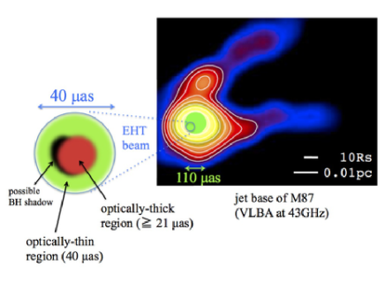
Figure 1.— Illustration of the jet base of M87 down to the EHT-region scale. The right panel shows the actual image of M87 with VLBA at 43 GHz adopted from Hada et al. (2013). The yellow-green circle shows the one-zone region with its diameter $110~{}{\rm\mu as}$ which is investigated in K14. The EHT-region detected by Doeleman et al. (2012) is shown as the blue circle. Since Hada et al. (2011) indicate that the central engine of M87 is located at $\sim 41~{}{\rm\mu as}$ eastward of the radio core at 43 GHz, we put the the EHT-region around there. The left panel shows the illustration of internal structure inside the EHT-region. The red-colored region represents an SSA-thick compact region inside the SSA-thin region. The black-colored region conceptually shows a possible BH shadow image. According to the smallness of closure phase reported in Akiyama et al. (2015), a certain level of symmetry is kept in this picture.

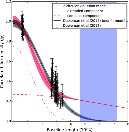
Figure 2.— Gaussian fittings to the correlated flux density of the M87 core obtained by EHT at 230 GHz. The flux density data plotted as a function of baseline length are adopted from Doeleman et al. (2012). The black solid curve is the best-fit circular Gaussian model with $S_{\nu}=0.98~{}{\rm Jy}$ and $\theta_{\rm FWHM}=40~{}{\rm\mu as}$ obtained by Doeleman et al. (2012). The red solid curve is the best-fit two-component model. The red dashed and dot-dashed curves represent the SSA-thick and the SSA-thin components, respectively. The SSA-thick component is expressed as the gaussian with $\theta_{\rm FWHM}=21~{}{\rm\mu as}/1.8=11.1~{}{\rm\mu as}$ and $S_{\nu}=0.27~{}{\rm Jy}$. The size and the flux density of the extended SSA-thin component are $\theta_{\rm FWHM}=60~{}{\rm\mu as}$ and $S_{\nu}=0.75~{}{\rm Jy}$. The blue-shaded region represents the baseline-length range corresponding to the one between the Hawaii/Arizona/California and Chile.

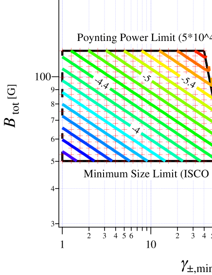
Figure 3.— The allowed region of $\gamma_{\pm,\rm min}$ and $B_{\rm tot}$ (the red cross points enclosed by the black trapezoid). The colored contour lines show the allowed $\log(U_{\pm}/U_{\rm B})$. The tags $\log(U_{\pm}/U_{\rm B})=$-4, -4.4, -5, and -5.4 are marked as reference values. The physical quantities and parameters adopted are $L_{\rm jet}=5\times 10^{44}~{}{\rm ergs^{-1}}$, and $p=3.0$. The minimum $\gamma_{\pm}$ is limited by $\nu_{\rm syn,\rm obs}$ at 230 GHz.

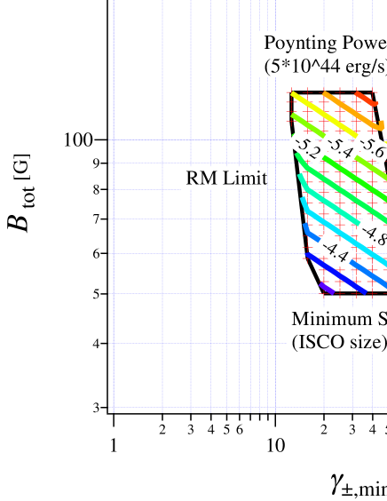
Figure 4.— The allowed region of $\gamma_{\pm,\rm min}$ and $B_{\rm tot}$ when $RM$ limit is taken into account. The physical quantities and parameters adopted are $L_{\rm jet}=5\times 10^{44}~{}{\rm ergs^{-1}}$, $p=3.0$, $\eta=0.99$ and $\zeta=m_{e}/m_{p}$ which corresponds to $e^{-}/p$-dominated composition with relativistic protons. The tags $\log(U_{\pm}/U_{\rm B})=$ -4.4, -4.8, -5.2, -5.4, and -5.6 are marked as reference values.

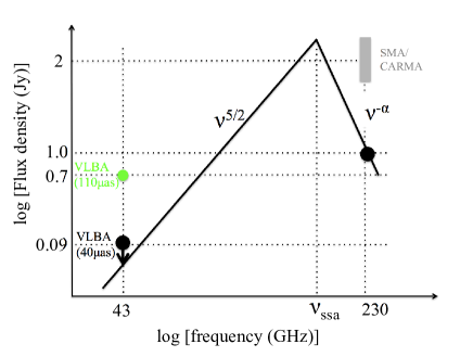
Figure 5.— Schematic view of synchrotron spectrum when the EHT-region is fully SSA-thin at 230 GHz with its size and flux density $40~{}{\rm\mu as}$ and 1.0 Jy (solid line). The upper limit on the flux density at 43 GHz is estimated as $0.09~{}{\rm Jy}=0.7~{}{\rm Jy}\times(40/110)^{2}$ based on the VLBA measurements of core size and flux at 43 GHz by Hada et al. (2013). The gray-colored range shows the typical flux density at 230 GHz obtained by SMA and CARMA (e.g., Doeleman et al. 2012; Kuo et al. 2014; Akiyama et al. 2015).

Table 1Results when the EHT region contains SSA-thick region

$L_{\rm j}$	allowed $B_{\rm tot}$	allowed $\theta_{\rm thick}$	allowed $U_{\pm}/U_{B}$
[erg s-1]	[G]	[$\mu$as]
$5\times 10^{44}$	$50\leq B_{\rm tot}\leq 124$	$21\leq\theta_{\rm thick}\leq 26.3$	$7.9\times 10^{-7}\leq\frac{U_{\pm}}{U_{B}}\leq 2.3\times 10^{-3}$

Table 2Results for the case of $e^{-}/p$-dominated composition with relativistic protons

$\eta$	$e^{+}$ fraction	$L_{\rm j}$	allowed $B_{\rm tot}$	allowed $\theta_{\rm thick}$	allowed $U_{\pm}/U_{B}$	allowed $U_{p}/U_{B}$
	[%]	[erg s-1]	[G]	[$\mu$as]
0.9	10	$5\times 10^{44}$	$50\leq B_{\rm tot}\leq 124$	$21\leq\theta_{\rm thick}\leq 26.3$	$7.9\times 10^{-7}\leq\frac{U_{\pm}}{U_{B}}\leq 1.1\times 10^{-4}$	$1.2\times 10^{-3}\leq\frac{U_{p}}{U_{B}}\leq 0.17$
0.99	1	$5\times 10^{44}$	$50\leq B_{\rm tot}\leq 124$	$21\leq\theta_{\rm thick}\leq 26.3$	$7.9\times 10^{-7}\leq\frac{U_{\pm}}{U_{B}}\leq 1.1\times 10^{-4}$	$1.4\times 10^{-3}\leq\frac{U_{p}}{U_{B}}\leq 0.20$
1	0	$5\times 10^{44}$	$50\leq B_{\rm tot}\leq 124$	$21\leq\theta_{\rm thick}\leq 26.3$	$7.9\times 10^{-7}\leq\frac{U_{\pm}}{U_{B}}\leq 1.1\times 10^{-4}$	$1.4\times 10^{-3}\leq\frac{U_{p}}{U_{B}}\leq 0.21$

Table 3Relevant coefficients for $B_{\perp}$ and $K_{\pm}$

$p$	$b(p)$	$b(p)$ in K14	$b(p)$ in Hirotani (2005)	$b(p)$ in Marscher (1983)	$k(p)$
2.5	$4.1\times 10^{-5}$	$3.3\times 10^{-5}$	$2.36\times 10^{-5}$	$3.6\times 10^{-5}$	$9.3\times 10^{-3}$
3.0	$2.4\times 10^{-5}$	$1.9\times 10^{-5}$	$2.08\times 10^{-5}$	$3.8\times 10^{-5}$	$1.4\times 10^{-3}$
3.5	$1.5\times 10^{-5}$	$1.2\times 10^{-5}$	$1.78\times 10^{-5}$	–	$2.1\times 10^{-4}$

References

- Abdo et al. (2009) Abdo, A. A., Ackermann, M., Ajello, M., et al. 2009, ApJ, 707, 55
- Akiyama et al. (2015) Akiyama, K., Lu, R-S., Fish, V. L., 2015, ApJ, submitted
- Alef et al. (2012) Alef, W., Anderson, J., Rottmann, H., et al. 2012, Proceedings of Science: 11th European VLBI Network Sympositum, Bordeax, France 10 Oct 2012,
- Amato & Arons (2006) Amato, E., & Arons, J. 2006, ApJ, 653, 325
- Asada et al. (2014) Asada, K., Nakamura, M., Doi, A., Nagai, H., & Inoue, M. 2014, ApJ, 781, L2
- Asada et al. (2009) Asada, K., Doi, A., Kino, M., et al. 2009, Approaching Micro-Arcsecond Resolution with VSOP-2: Astrophysics and Technologies, 402, 262
- Asano & Takahara (2009) Asano, K., & Takahara, F. 2009, ApJ, 690, L81
- Begelman et al. (1984) Begelman, M. C., Blandford, R. D., & Rees, M. J. 1984, Reviews of Modern Physics, 56, 255
- Bessho & Bhattacharjee (2007) Bessho, N., & Bhattacharjee, A. 2007, Physics of Plasmas, 14, 056503
- Bessho & Bhattacharjee (2012) Bessho, N., & Bhattacharjee, A. 2012, ApJ, 750, 129
- Bicknell & Begelman (1996) Bicknell, G. V., & Begelman, M. C. 1996, ApJ, 467, 597
- Blakeslee et al. (2009) Blakeslee, J. P., Jordán, A., Mei, S., et al. 2009, ApJ, 694, 556
- Blandford & Payne (1982) Blandford, R. D., & Payne, D. G. 1982, MNRAS, 199, 883
- Blandford & Rees (1978) Blandford, R. D., & Rees, M. J. 1978, Phys. Scr, 17, 265
- Blandford & Znajek (1977) Blandford, R. D., & Znajek, R. L. 1977, MNRAS, 179, 433
- Broderick & McKinney (2010) Broderick, A. E., & McKinney, J. C. 2010, ApJ, 725, 750
- Broderick & Loeb (2009) Broderick, A. E., & Loeb, A. 2009, ApJ, 697, 1164
- Burbidge et al. (1974) Burbidge, G. R., Jones, T. W., & Odell, S. L. 1974, ApJ, 193, 43
- Chandrasekhar (1967) Chandrasekhar, S. 1967, An Introduction to the Study of Stellar Structure (New York: Dover)
- Chiueh et al. (1991) Chiueh, T., Li, Z.-Y., & Begelman, M. C. 1991, ApJ, 377, 462
- Cotton et al. (1980) Cotton, W. D., Wittels, J. J., Shapiro, I. I., et al. 1980, ApJ, 238, L123
- Despringre et al. (1996) Despringre, V., Fraix-Burnet, D., & Davoust, E. 1996, A&A, 309, 375
- Dexter et al. (2012) Dexter, J., McKinney, J. C., & Agol, E. 2012, MNRAS, 421, 1517
- Dodson et al. (2013) Dodson, R., Rioja, M., Asaki, Y., et al. 2013, AJ, 145, 147
- Dodson et al. (2006) Dodson, R., Edwards, P. G., & Hirabayashi, H. 2006, PASJ, 58, 243
- Doeleman et al. (2012) Doeleman, S. S., Fish, V. L., Schenck, D. E., et al. 2012, Science, 338, 355
- Doeleman et al. (2009) Doeleman, S. S., Fish, V. L., Broderick, A. E., Loeb, A., & Rogers, A. E. E. 2009, ApJ, 695, 59
- Doi et al. (2013) Doi, A., Hada, K., Nagai, H., et al. 2013, The Innermost Regions of Relativistic Jets and Their Magnetic Fields, Granada, Spain, Edited by Jose L. Gomez; EPJ Web of Conferences, European Physical Journal Web of Conferences, 61, 8008
- Falcke et al. (2000) Falcke, H., Melia, F., & Agol, E. 2000, ApJ, 528, L13
- Fish et al. (2013) Fish, V., Alef, W., Anderson, J., et al. 2013, High-Angular-Resolution and High-Sensitivity Science Enabled by Beamformed ALMA, (arXiv:1309.3519)
- Fish et al. (2011) Fish, V. L., Doeleman, S. S., Beaudoin, C., et al. 2011, ApJ, 727, LL36
- Gebhardt & Thomas (2009) Gebhardt, K., & Thomas, J. 2009, ApJ, 700, 1690
- Ginzburg & Syrovatskii (1965) Ginzburg, V. L., & Syrovatskii, S. I. 1965, ARA&A, 3, 297 (GS65)
- Hada et al. (2014) Hada, K., Giroletti, M., Kino, M., et al. 2014, ApJ, 788, 165
- Hada et al. (2013) Hada, K., Kino, M., Doi, A., et al. 2013a, ApJ, 775, 70
- Hada et al. (2011) Hada, K., Doi, A., Kino, M., et al. 2011, Nature, 477, 185
- Hirotani (2005) Hirotani, K. 2005, ApJ, 619, 73
- Honma et al. (2014) Honma, M., Akiyama, K., Uemura, M., & Ikeda, S. 2014, PASJ, 66, 95
- Hoshino (2013) Hoshino, M. 2013, ApJ, 773, 118
- Hoshino & Arons (1991) Hoshino, M., & Arons, J. 1991, Physics of Fluids B, 3, 818
- Iwamoto & Takahara (2002) Iwamoto, S., & Takahara, F. 2002, ApJ, 565, 163
- Jones & Odell (1977) Jones, T. W., & Odell, S. L. 1977, ApJ, 214, 522
- Jones et al. (1974) Jones, T. W., O’dell, S. L., & Stein, W. A. 1974a, ApJ, 192, 261
- Jones et al. (1974) Jones, T. W., O’dell, S. L., & Stein, W. A. 1974b, ApJ, 188, 353
- Jordán et al. (2005) Jordán, A., Côté, P., Blakeslee, J. P., et al. 2005, ApJ, 634, 1002
- Junor et al. (1999) Junor, W., Biretta, J. A., & Livio, M. 1999, Nature, 401, 891
- Kato et al. (1998) Kato, S., Fukue, J., & Mineshige, S. 1998, Black-hole Accretion Disks (Kyoto: Kyoto Univ. Press)
- Kellermann & Pauliny-Toth (1969) Kellermann, K. I., & Pauliny-Toth, I. I. K. 1969, ApJ, 155, L71
- Kimura et al. (2014) Kimura, S. S., Toma, K., & Takahara, F. 2014, ApJ, 791, 100
- Kino et al. (2014) Kino, M., Takahara, F., Hada, K., & Doi, A. 2014, ApJ, 786, 5 (K14)
- Kino et al. (2012) Kino, M., Kawakatu, N., & Takahara, F. 2012, ApJ, 751, 101
- Kirk & Skjæraasen (2003) Kirk, J. G., & Skjæraasen, O. 2003, ApJ, 591, 366
- Koide et al. (2002) Koide, S., Shibata, K., Kudoh, T., & Meier, D. L. 2002, Science, 295, 1688
- Komissarov et al. (2009) Komissarov, S. S., Vlahakis, N., Konigl, A., & Barkov, M. V. 2009, MNRAS, 394, 1182
- Komissarov et al. (2007) Komissarov, S. S., Barkov, M. V., Vlahakis, N., Konigl, A. 2007, MNRAS, 380, 51
- Krichbaum et al. (2006) Krichbaum, T. P., Graham, D. A., Bremer, M., et al. 2006, Journal of Physics Conference Series, 54, 328
- Krolik et al. (2005) Krolik, J. H., Hawley, J. F., & Hirose, S. 2005, ApJ, 622, 1008
- Kuo et al. (2014) Kuo, C. Y., Asada, K., Rao, R., et al. 2014, ApJ, 783, LL33
- Le & Becker (2004) Le, T., & Becker, P. A. 2004, ApJ, 617, L25
- Lee (2013) Lee, S.-S. 2013, Journal of Korean Astronomical Society, 46, 243
- Li et al. (1992) Li, Z.-Y., Chiueh, T., & Begelman, M. C. 1992, ApJ, 394, 459
- Loeb & Waxman (2007) Loeb, A., & Waxman, E. 2007, JCAP, 3, 011
- Lu et al. (2014) Lu, R.-S., Broderick, A. E., Baron, F., et al. 2014, ApJ, 788, 120
- Lu et al. (2012) Lu, R.-S., Fish, V. L., Weintroub, J., et al. 2012, ApJ, 757, LL14
- Macchetto et al. (1997) Macchetto, F., Marconi, A., Axon, D. J., et al. 1997, ApJ, 489, 579
- Manmoto et al. (1997) Manmoto, T., Mineshige, S., & Kusunose, M. 1997, ApJ, 489, 791
- Marscher (1987) Marscher, A. P. 1987, Superluminal Radio Sources (Cambridge: Cambridge Univ. Press), 280
- Marscher (1983) Marscher, A. P. 1983, ApJ, 264, 296 (M83)
- Marscher (1977) Marscher, A. P. 1977, AJ, 82, 781
- McKinney et al. (2013) McKinney, J. C., Tchekhovskoy, A., & Blandford, R. D. 2013, Science, 339, 49
- McKinney (2006) McKinney, J. C. 2006, MNRAS, 368, 1561
- McKinney & Gammie (2004) McKinney, J. C., & Gammie, C. F. 2004, ApJ, 611, 977
- Mizuta et al. (2010) Mizuta, A., Kino, M., & Nagakura, H. 2010, ApJ, 709, L83
- Nagakura & Takahashi (2010) Nagakura, H., & Takahashi, R. 2010, ApJ, 711, 222
- Nakamura & Asada (2013) Nakamura, M., & Asada, K. 2013, 775, 118
- Okamoto (1999) Okamoto, I. 1999, MNRAS, 307, 253
- Okamoto (1974) Okamoto, I. 1974, MNRAS, 167, 457
- Owen et al. (2000) Owen, F. N., Eilek, J. A., & Kassim, N. E. 2000, ApJ, 543, 611
- Owen et al. (1978) Owen, F. N., Porcas, R. W., Mufson, S. L., & Moffett, T. J. 1978, AJ, 83, 685
- Pacholczyk (1970) Pacholczyk, A. G. 1970, Series of Books in Astronomy and Astrophysics, San Francisco: Freeman, 1970,
- Quataert & Gruzinov (2000) Quataert, E., & Gruzinov, A. 2000, ApJ, 545, 842
- Reynolds et al. (1996) Reynolds, C. S., Fabian, A. C., Celotti, A., & Rees, M. J. 1996, MNRAS, 283, 873
- Rieger & Aharonian (2012) Rieger, F. M., & Aharonian, F. 2012, Modern Physics Letters A, 27, 30030
- Rioja & Dodson (2011) Rioja, M., & Dodson, R. 2011, AJ, 141, 114
- Rybicki & Lightman (1979) Rybicki, G. B., & Lightman, A. P. 1979, New York, Wiley-Interscience, 1979
- Sari et al. (1998) Sari, R., Piran, T., & Narayan, R. 1998, ApJ, 497, L17
- Slysh (1992) Slysh, V. I. 1992, ApJ, 391, 453
- Spruit (2010) Spruit, H. C. 2010, Lecture Notes in Physics, Berlin Springer Verlag, 794, 233
- Stawarz et al. (2006) Stawarz, Ł., Aharonian, F., Kataoka, J., et al. 2006, MNRAS, 370, 981
- Takahashi & Mineshige (2011) Takahashi, R., & Mineshige, S. 2011, ApJ, 729, 86
- Takahashi (2004) Takahashi, R. 2004, ApJ, 611, 996
- Takamoto et al. (2012) Takamoto, M., Inoue, T., & Inutsuka, S.-i. 2012, ApJ, 755, 76
- Tan et al. (2008) Tan, J. C., Beuther, H., Walter, F., & Blackman, E. G. 2008, ApJ, 689, 775
- Tchekhovskoy et al. (2011) Tchekhovskoy, A., Narayan, R., & McKinney, J. C. 2011, MNRAS, 418, L79
- Thompson et al. (2001) Thompson, A. R., Moran, J. M., & Swenson, G. W., Jr. 2001, ”Interferometry and synthesis in radio astronomy by A. Richard Thompson, James M. Moran, and George W. Swenson, Jr. 2nd ed. New York : Wiley, (ISBN : 0471254924”)
- Toma & Takahara (2013) Toma, K., & Takahara, F. 2013, PTEP, 2013, 080003
- Toma & Takahara (2012) Toma, K., & Takahara, F. 2012, ApJ, 754, 148
- Tomimatsu & Takahashi (2003) Tomimatsu, A., & Takahashi, M. 2003, ApJ, 592, 321
- Tsang & Kirk (2007) Tsang, O., & Kirk, J. G. 2007, A&A, 476, 1151
- Uchida (1997) Uchida, T. 1997, Phys. Rev. E, 56, 2181
- Ulvestad & Ho (2001) Ulvestad, J. S., & Ho, L. C. 2001, ApJ, 558, 561
- Vlahakis Konigl (2003) Vlahakis, N., Konigl, A. 2003, ApJ, 596, 1080
- Walsh et al. (2013) Walsh, J. L., Barth, A. J., Ho, L. C., & Sarzi, M. 2013, ApJ, 770, 86
- Young et al. (2002) Young, A. J., Wilson, A. S., & Mundell, C. G. 2002, ApJ, 579, 560
- Zavala & Taylor (2004) Zavala, R. T., & Taylor, G. B. 2004, ApJ, 612, 749