Abstract

We study a catalytic branching process (CBP) with any finite set of catalysts. This model describes a system of particles where the movement is governed by a Markov chain with arbitrary finite or countable state space and the branching may only occur at the points of catalysis. The results obtained generalize and strengthen those known in cases of CBP with a single catalyst and of branching random walk on ${\bf Z}^{d}$, $d\in{\bf N}$, with a finite number of sources of particles generation. We propose to classify CBP with $N$ catalysts as supercritical, critical or subcritical according to the value of the Perron root of a specified $N\times N$ matrix. Such classification agrees with the moment analysis performed here for local and total particles numbers. By introducing the criticality set $C$ we also consider the influence of catalysts parameters on the process behavior. The proof is based on construction of auxiliary multi-type Bellman-Harris processes with the help of hitting times under taboo and on application of multidimensional renewal theorems.

Keywords and phrases: catalytic branching process, classification, hitting times under taboo, moment analysis, multi-type Bellman-Harris process.

2010 AMS classification: 60J80, 60J27.

1 Introduction

We consider the model of catalytic branching process (CBP) with a finite number of catalysts. It describes a system of particles moving in space and branching only in the presence of catalysts. More exactly, let at the initial time $t=0$ there be a single particle that moves on some finite or countable set $S$ according to a continuous-time Markov chain $\eta=\{\eta(t),t\geq 0\}$ generated by infinitesimal matrix $Q=(q(x,y))_{x,y\in S}$. When this particle hits a finite set of catalysts ${W=\{w_{1},\ldots,w_{N}\}\subset S}$, say at the site $w_{k}$, it spends there random time having the exponential distribution with parameter $\beta_{k}>0$. Afterwards the particle either branches or leaves the site $w_{k}$ with probabilities $\alpha_{k}$ and $1-\alpha_{k}$ ($0\leq\alpha_{k}<1$), respectively. If the particle branches (at the site $w_{k}$), it dies and just before the death produces a random non-negative integer number $\xi_{k}$ of offsprings located at the same site $w_{k}$. If the particle leaves $w_{k}$, it jumps to the site $y\neq w_{k}$ with probability $-(1-\alpha_{k})q(w_{k},y)q(w_{k},w_{k})^{-1}$ and continues its movement governed by the Markov chain $\eta$. All newly born particles are supposed to behave as independent copies of their parent.

We assume that the Markov chain $\eta$ is irreducible and the matrix $Q$ is conservative (i.e. $\sum\nolimits_{y\in S}{q(x,y)}=0$ where $q(x,y)\geq 0$ for $x\neq y$ and $q(x,x)\in(-\infty,0)$ for any $x\in S$). Denote by $f_{k}(s):={\sf E}{s^{\xi_{k}}}$, $s\in[0,1]$, the probability generating function of $\xi_{k}$, $k=1,\ldots,N$. We will employ the standard assumption of existence of a finite derivative $f_{k}^{\prime}(1)$, that is the finiteness of ${\bf E}{\xi_{k}}$, for any $k=1,\ldots,N$.

Study of CBP with a single catalyst was initiated even in the XX century (see, e.g., [2]). In this regard we also mention a recent paper [14] where the main tool for the moment analysis of the process was the spine technique, i.e. “many-to-few lemma”, and renewal theory. Note that the generalization to an arbitrary finite set of catalysts is not straightforward, since there exists a ”competition” between catalysts. An important special case of several catalysts (where $S={\bf Z}^{d}$, $d\in{\bf N}$, and the Markov chain $\eta$ is symmetric space-homogeneous random walk with finite variance of jump sizes) was examined in [33]. There the sufficient conditions for exponential growth of the particles numbers were obtained by analyzing spectral properties of evolution operators. We propose another way permitting to establish more precise results.

For branching processes the natural interesting problem is the analysis of asymptotic behavior (as $t\to\infty$) of the local and total size of population at time $t$ (for various branching processes without catalysts see, e.g., [27]). Let $\mu(t)$ stand for the total number of particles existing in CBP at time $t\geq 0$. In a similar way we define local numbers $\mu(t;y)$ as quantities of particles located at separate points $y\in S$ at time $t$. In this paper our aim is three-fold. Firstly, we introduce a classification of CBP (with $N$ catalysts) treating it as supercritical, critical or subcritical whenever one has, for the Perron root $\rho$ of a certain $N\times N$ matrix, $\rho>1$, $\rho=1$ or $\rho<1$, respectively. Moreover, the criticality set $C$ revealing the influence of catalysts strength is introduced and characterized. Secondly, we implement the moment analysis of the local and total particles numbers to justify the naturalness of the proposed classification (indeed, one will see that the asymptotic behavior of the moments of any order is determined essentially by the introduced class of CBP). Thirdly, we consider some particular cases of CBP and thereby show that our study not only generalizes the results in previous works but even refines them.

Our approach consists in involving hitting times under taboo (see, e.g., [6], [9] and [11], Ch.2, Sec.11) and construction of auxiliary Bellman-Harris branching processes with at most $N(N+1)+1$ types of particles. This approach is inspired by [31] where the branching random walk on ${\bf Z}$ with a single catalyst was investigated by means of introducing hitting times (without taboo) and a due two-type Bellman-Harris process. Note also that in [10], for the study of a discrete-time branching random walk on ${\bf Z}$ with multiple catalysts, the authors considered an embedded multi-type Galton-Watson branching process, resulting in ”forgetting/erasing the time spent between catalysts”. The latter approach is fruitful for classification of branching random walk since multi-type Galton-Watson and multi-type Bellman-Harris processes have the same supercritical, critical or subcritical regimes. However, for subsequent study of branching random walks (moment analysis, limit theorems etc.) multi-type Galton-Watson process is not sufficient and thus Ph.Carmona and Y.Hu used in [10] another technique such as ”many-to-few lemmas”. Our first auxiliary process is constructed in such a way that the study of CBP can be mainly reduced to analysis of the Bellman-Harris process. The number of particles in this process is chosen to guarantee its indecomposability and cannot be less than $N$ and need not be greater than $N(N+1)$. It is well-known (see, e.g., [27], Ch.4, Sec.5, 6 and 7) that an indecomposable multi-type Bellman-Harris process is classified as supercritical, critical or subcritical according to the value of the Perron root of the mean matrix. This is the foundation for classification of CBP. Furthermore, Lemma 1 below gives even more convenient classification with the help of the Perron root of a specified irreducible $N\times N$ matrix. One more auxiliary Bellman-Harris process is indispensable for study of total particles numbers in CBP in case of transient Markov chain $\eta$. This process is taken to be decomposable with a final type of particles. The treatment of the auxiliary Bellman-Harris processes allows us not only to classify CBP but also to derive a system of renewal equations for the mean local and total particles numbers in CBP. Afterwards, to implement the moment analysis of the local and total particles numbers we use multidimensional renewal theorems established in [12] and [23].

This approach has advantages since there is elaborated theory of multi-type Bellman-Harris processes and a vast majority of its results can be applied to the auxiliary Bellman-Harris processes leading to the new results for CBP. Mention in passing some recent works on multi-type Bellman-Harris processes, see, e.g., [18], [30] and [32].

Observe also that CBP can be considered as a Markov branching process with at most countably many types of particles, since the location of a particle can be associated with its type. Theory of branching processes with countably many types of particles, despite of its long history (see, e.g., [24]), has not been systematized until now in view of its complexity. Some new papers such as [3], [4], [16] and [25] make an important contribution to this research direction. However, the study there does not cover the results presented in our paper. Among other investigations of models describing particles movement and breeding we refer to recent papers [5], [17] and [21]. Branching random walks analyzed there are homogeneous in space whereas the main feature of CBP is spatial non-homogeneity. Some differences in behavior of a homogeneous branching random walk on ${\bf Z}$ and its catalytic counterpart are discussed in [10]. Concluding the introduction we mention the close relation between a catalytic branching random walk on ${\bf Z}$ and a super-Brownian motion with a single point catalyst (see, e.g., [13] and [15]).

Now we describe the structure of the paper. In section 2 we specify the first auxiliary Bellman-Harris process and propose a classification for CBP. Section 3 is devoted to solution of the following problem. Assume that we fix the Markov chain generator $Q$ in CBP and vary “intensities” of catalysts, e.g., ${m_{k}:={\sf E}{\xi_{k}}}$, $k=1,\ldots,N$. What is the set $C\subset{\bf R}^{N}_{+}$ such that CBP is critical iff ${m=(m_{1},\ldots,m_{N})\in C}$? In particular, what is the proportion of “weak” and “powerful” catalysts (possessing small or large values of $m_{i}$, respectively) in critical regime? In section 3 we obtain a complete description of $C$ by means of equation involving determinants of some matrices, indicate the smallest parallelepiped $[0,M_{1}]\times\ldots\times[0,M_{N}]$ containing $C$ and illustrate our approach by two pictures of the set $C$ when $N=2$ and $N=3$. Observe that these plots are not a product of simulation and display the result of direct computation. Section 4 contains Theorem 1 and its proof representing the moment analysis of the local and total particles numbers in CBP. There we construct the second auxiliary Bellman-Harris process required for study of the total size of population whenever Markov chain $\eta$ is transient. Section 5 demonstrates applications of our results to the catalytic branching random walk on ${\bf Z}^{d}$ and to the branching process with a single catalyst. A detailed comparison of our results with those known before is given as well.

2 Auxiliary Bellman-Harris process

Let us briefly describe a Bellman-Harris branching process with particles of $n$ types, $n\in{\bf N}$. It is initiated by a single particle of type $i=1,\ldots,n$. The parent particle has a random life-length with a cumulative distribution function (c.d.f.) $G_{i}(t)$, $t\geq 0$. When dying the particle produces offsprings according to a probability generating function $g_{i}({\bf s})$, ${\bf s}=(s_{1},\ldots,s_{n})\in[0,1]^{n}$. The new particles of type ${j=1,\ldots,n}$ evolve independently with the life-length distribution $G_{j}(\cdot)$ and an offspring generating function $g_{j}(\cdot)$. Let

$$M:=\left(m_{i,j}\right)_{i,j=1}^{n}\;\;\mbox{with}\;\;m_{i,j}=\left.\partial_{s_{j}}g_{i}\right|_{{\bf s}=(1,\ldots,1)}$$

be the mean matrix of the process. The Bellman-Harris branching process is called indecomposable if the non-negative matrix $M$ is irreducible (for the latter notion, see, e.g., [26], Ch.1, Sec.3). Moreover, if its Perron root $\rho$ (i.e. eigenvalue having the maximal modulus) is such that $\rho>1$, $\rho=1$ or $\rho<1$, then the Bellman-Harris process is called supercritical, critical or subcritical, respectively (see, e.g., [27], Ch.4, Sec.5, 6 and 7). Denote the number of particles of type $j$ existing at time $t$ by $Z_{j}(t)$, $t\geq 0$, $j=1,\ldots,n$.

Before demonstrating how an auxiliary Bellman-Harris process can be constructed in the framework of CBP we have to introduce some notation. Consider a particle moving on the set $S$ in accordance with the Markov chain generated by $Q$ and starting at state $x$. Let ${}_{H}\overline{\tau}_{x,y}$, $x,y\in S$, $H\subset S$, be the time spent by the particle after leaving the starting point $x$ until the first hitting $y$ if the particle’s trajectory does not pass $H$. Otherwise (if the particle’s trajectory passes $H$ before the first hitting $y$), ${{}_{H}\overline{\tau}_{x,y}=\infty}$. The (extended) random variable ${}_{H}\overline{\tau}_{x,y}$ is called a hitting time of state $y$ under taboo $H$ after the first exit out of the starting state $x$. Denote by ${}_{H}\overline{F}_{x,y}(t)$, $t\geq 0$, the improper c.d.f. of ${}_{H}\overline{\tau}_{x,y}$. Evidently, ${{}_{H}\overline{F}_{x,y}(0)=(\delta_{x,y}-1)q(x,y)q(x,x)^{-1}}$ where $\delta_{x,y}$ is the Kronecker delta. Explicit formulae for the probability of finiteness of ${}_{H}\overline{\tau}_{x,y}$, i.e. for ${}_{H}\overline{F}_{x,y}(\infty)=\lim\nolimits_{t\to\infty}{{}_{H}\overline{F}_{x,y}(t)}$, via taboo probabilities and Green’s function were derived in [9]. Whenever the taboo set $H$ is empty we write $\overline{\tau}_{x,y}$ and $\overline{F}_{x,y}(\cdot)$ instead of ${{}_{\emptyset}\overline{\tau}_{x,y}}$ and ${{}_{\emptyset}\overline{F}_{x,y}(\cdot)}$, respectively.

Return to CBP. We tentatively assume that CBP starts at $w_{p}$ for some ${p=1,\ldots,N}$. Set $K_{j}:=\{k=1,\ldots,N:{{}_{W_{k}}\overline{F}}_{w_{j},w_{k}}(\infty)-{{}_{W_{k}}\overline{F}_{w_{j},w_{k}}}(0)>0\}$ for $W_{k}:=W\setminus\{w_{k}\}$ and $j=1,\ldots,N$. Let $K_{j}=\{k(1,j),\ldots,k(|K_{j}|,j)\}$ where $1\leq k(1,j)<k(2,j)<\ldots<k(|K_{j}|,j)\leq N$ and $|\cdot|$ is the cardinality of a finite set. We divide the particles population existing at time $t\geq 0$ into $L+1$ groups with $L:=N+\sum\nolimits_{j=1}^{N}{|K_{j}|}$. The particles located at time $t$ at $w_{j}$ form the $j$-th group having cardinality $\mu(t;w_{j})$, $j=1,\ldots,N$. Consider a family consisting of particles which have left $w_{j}$ at least once within time interval $[0,t]$, upon the last leaving $w_{j}$ have not yet reached $W$ by time $t$ but eventually will hit $w_{k(i,j)}$ before possible hitting $W_{k(i,j)}$, $i=1,\ldots,|K_{j}|$, $j=1,\ldots,N$. This family has cardinality denoted by $\mu_{j,i}(t)$ and corresponds to the group number $(L(j)+i)$ where $L(j):=N+\sum\nolimits_{l=1}^{j-1}{|K_{l}|}$. The group number $L+1$ comprises the rest of particles not included into the above $L$ groups. Note that the last group consists of the particles having infinite life-lengths since after time $t$ they will not hit the set of catalysts any more. So, after time $t$ these particles will not produce any offsprings and have no influence on the numbers of particles in other $L$ groups.

Now we can introduce an auxiliary Bellman-Harris process to employ it for the study of CBP. Consider an $L$-dimensional Bellman-Harris process starting with a single particle of type $p$ and having the following c.d.f. and offspring generating functions

$$G_{j}(t)=1-e^{-\beta_{j}t},\quad g_{j}({\bf s})=\alpha_{j}f_{j}(s_{j})+(1-\alpha_{j})\sum\limits_{k=1}^{N}{{}_{W_{k}}\overline{F}_{w_{j},w_{k}}(0)s_{k}}$$ (1)

$$+(1-\alpha_{j})\!\sum\limits_{i=1}^{|K_{j}|}T_{i,j}(\infty)s_{L(j)+i}+(1-\alpha_{j})\left(1-\sum\limits_{k=1}^{N}{{}_{W_{k}}\overline{F}_{w_{j},w_{k}}(\infty)}\right),$$

$$G_{L(j)+i}(t)=\frac{T_{i,j}(t)}{T_{i,j}(\infty)},\quad g_{L(j)+i}({\bf s})=s_{k(i,j)}$$ (2)

where $T_{i,j}(t):={{}_{W_{k(i,j)}}\overline{F}_{w_{j},w_{k(i,j)}}(t)}-{{}_{W_{k(i,j)}}\overline{F}_{w_{j},w_{k(i,j)}}(0)}$, $0\leq t\leq\infty$ and $i=1,\ldots,|K_{j}|$, $j=1,\ldots,N$. It is easy to see that for the process constructed in this way the vector $(Z_{1}(t),\ldots,Z_{L}(t))$, at each $t\geq 0$, has the same distribution as the vector whose $j$-th component is $\mu(t;w_{j})$ and $(L(j)+i)$-th component is $\mu_{j,i}(t)$, $i=1,\ldots,|K_{j}|$, $j=1,\ldots,N$.

Mean matrix $M=(m_{k,l})_{k,l=1}^{L}$ of the introduced Bellman-Harris process is of block form, i.e.

$$M=\left(\begin{array}[]{cccc}M_{1,1}&M_{1,2}&\ldots&M_{1,N+1}\\ M_{2,1}&M_{2,2}&\ldots&M_{2,N+1}\\ \ldots&\ldots&\ldots&\ldots\\ M_{N+1,1}&M_{N+1,2}&\ldots&M_{N+1,N+1}\\ \end{array}\right).$$ (3)

Here the $N\times N$ matrix $M_{1,1}=(m_{k,l})_{k,l=1}^{N}$ possesses the following entries $m_{k,l}=\delta_{k,l}\,\alpha_{k}f^{\prime}_{k}(1)+(1-\alpha_{k}){{}_{W_{l}}\overline{F}_{w_{k},w_{l}}}(0)$. For $j=1,\ldots,N$, the elements of $N\times|K_{j}|$ matrix $M_{1,j+1}$ vanish everywhere except for the $j$-th row and for ${i=1,\ldots,|K_{j}|}$ one has $m_{j,L(j)+i}=(1-\alpha_{j})T_{i,j}(\infty)$. When $i=1,\ldots,N$ the $|K_{i}|\times N$ matrix $M_{i+1,1}$ is such that omitting its $j$-th null columns for all $j\notin K_{i}$ one gets the $|K_{i}|\times|K_{i}|$ identity matrix. For $i,j=1,\ldots,N$, the $|K_{i}|\times|K_{j}|$ matrices $M_{i+1,j+1}$ have zero entries.

Let us verify that the specified Bellman-Harris process is indecomposable. In view of irreducibility of the Markov chain $\eta$ there exists a finite path from $w_{k}$ to $w_{l}$ with a positive probability for each $k,l=1,\ldots,N$. In the framework of CBP such path has also positive probability, since being at catalyst site $w_{i}$ a particle can leave it without branching with positive probability $1-\alpha_{i}$ for each $i=1,\ldots,N$. Among the sites visited successively by that path of $\eta$ choose those from $W$, say, $w_{p(0)},w_{p(1)},\ldots,w_{p(J)},w_{p(J+1)}$ with $p(0)\!:=k$ and ${p(J+1)\!:=l}$. By the construction of auxiliary Bellman-Harris process this path corresponds to transformations of a particle type from $k$ to $l$. Namely, if the path of $\eta$ hits $w_{p(j+1)}$ immediately after leaving $w_{p(j)}$ then the particle type in Bellman-Harris process changes from $p(j)$ to $p(j+1)$. Otherwise, $p(j+1)\in K_{p(j)}$, i.e. $p(j+1)=k(i,p(j))$ for some $i=1,\ldots,|K_{p(j)}|$, and the particle type change from $p(j)$ to $p(j+1)$ involves the intermediate type $L(p(j))+i$. Hence, we conclude that, for each $k$ and $l$ from $\{1,\ldots,N\}$, there exists $n=n(k,l)\in{\bf N}$ and a collection $\{r(1),\ldots,r(n)\}\subset\{1,\ldots,L\}$ such that $m_{k,r(1)}m_{r(1),r(2)}\ldots m_{r(n),l}>0$. Since by matrix $M$ definition in (3) one has $m_{L(j)+i,k(i,j)}=1>0$ and $m_{j,L(j)+i}>0$ for each $i=1,\ldots,|K_{j}|$ and $j=1,\ldots,N$, the previous statement holds true for $k,l=1,\ldots,L$ as well. Consequently, we have checked that for each $k$ and $l$ from $\{1,\ldots,L\}$, there exists $n=n(k,l)\in{\bf N}$ such that $m^{(n)}_{k,l}>0$ where $m^{(n)}_{k,l}$ is the $(k,l)$-th element of $M^{n}$. So, we have verified that the matrix $M$ is irreducible. Moreover, if we consider the nontrivial case $f_{i}^{\prime}(1)>0$ for some $i=1,\ldots,N$, then $m_{i,i}>0$ and the matrix $M$ is acyclic (or aperiodic) (see, e.g., [26], Ch.1, Sec.2). Thereby, in this case we have shown that $M$ is a primitive matrix (see, e.g., [26], Ch.1, Sec.3).

On account of the Perron-Frobenius theorem for irreducible matrices (see, e.g., [26], Ch.1, Sec.4) the matrix $M$ has a positive real eigenvalue $\rho(M)$ of maximal modulus which is called the Perron root of $M$. Using the classification of the constructed Bellman-Harris process we call CBP supercritical, critical or subcritical if $\rho(M)>1$, $\rho(M)=1$ or $\rho(M)<1$, respectively, where $M$ is specified by (3). Since $M$ is independent of the CBP starting point, the same is true for the classification of CBP. So, from here on we omit our assumption that CBP starts at some $w_{p}\in W$.

Let $G^{\ast}_{i}(\lambda):=\int\nolimits_{0-}^{\infty}{e^{-\lambda t}\,dG_{i}(t)}$, $\lambda\geq 0$, be the Laplace-Stieltjes transform of c.d.f. $G_{i}$ and $H(\lambda):=\left(G^{\ast}_{i}(\lambda)m_{i,j}\right)_{i,j=1}^{L}$. Note that $H(0)=M$. Matrix $H(\lambda)$ is irreducible in view of irreducibility of $M$. Put also $D(\lambda)=(d_{i,j}(\lambda))_{i,j=1}^{N}$, $\lambda\geq 0$, with $d_{i,j}(\lambda):=\delta_{i,j}\,\alpha_{i}f_{i}^{\prime}(1)G^{\ast}_{i}(\lambda)+(1-\alpha_{i})G^{\ast}_{i}(\lambda){{}_{W_{j}}\overline{F}^{\ast}_{w_{i},w_{j}}(\lambda)}$. It is easily seen that the matrix $D=(d_{i,j})_{i,j=1}^{N}$ defined as $D:=D(0)$ has entries

$${d_{i,j}=\delta_{i,j}\,\alpha_{i}f_{i}^{\prime}(1)+(1-\alpha_{i}){{}_{W_{j}}\overline{F}_{w_{i},w_{j}}(\infty)}}.$$ (4)

For an irreducible matrix $A$, let $\rho(A)$ stand for the Perron root of $A$. The following statement gives a convenient criticality condition for CBP.

Lemma 1

For each $\lambda\geq 0$, the matrix $D(\lambda)$ is irreducible and the values $\rho(D(\lambda))$ and $\rho(H(\lambda))$ are simultaneously greater than $1$, equal to $1$ or less than $1$. In particular, the Perron roots $\rho(D)$ and $\rho(M)$ are either both greater than $1$, or equal to $1$, or are less than $1$.

Proof. The irreducibility of $D$ (and, therefore, of $D(\lambda)$) is established in the same manner as for matrix $M$. In accordance with the Perron-Frobenius theorem matrix $H(\lambda)$ has a strictly positive left eigenvector ${\bf v}$ corresponding to the eigenvalue $\rho(H(\lambda))$. Consequently, $H(\lambda)^{\top}{\bf v}=\rho(H(\lambda)){\bf v}$ where $\top$ means transposition and ${\bf v}$ is considered as a column vector. In other words, $\left(H(\lambda)^{\top}-\rho(H(\lambda))I\right){\bf v}={\bf 0}$ for $I$ being the identity matrix and ${\bf 0}$ standing for the zero of ${\bf R}^{L}$. Apply some equivalent transformations to the obtained system of equations, namely, for each ${j,k=1,\ldots,N}$ add the $(L(j)+i)\mbox{-th}$ row multiplied by $G^{\ast}_{L(j)+i}(\lambda)\rho(H(\lambda))^{-1}$ to the $k$-th row if $k\in K_{j}$, i.e. ${k=k(i,j)}$ for some $i=1,\ldots,|K_{j}|$. Focusing on the first $N$ equations only, we deduce that

$${\bf v}_{0}^{\top}\left(H_{1,1}(\lambda)+\rho(H(\lambda))^{-1}R(\lambda)-\rho(H(\lambda))I\right)={\bf 0}^{\top}.$$

Here we denote $H_{1,1}(\lambda):=(G^{\ast}_{i}(\lambda)m_{i,j})_{i,j=1}^{N}$ and matrix $R(\lambda):=(r_{i,j}(\lambda))_{i,j=1}^{N}$ has the following entries ${r_{i,j}(\lambda):=(1-\alpha_{i})G^{\ast}_{i}(\lambda)\left({{}_{W_{j}}}\overline{F}^{\ast}_{w_{i},w_{j}}(\lambda)-{{}_{W_{j}}}\overline{F}_{w_{i},w_{j}}(0)\right)}$ whereas ${\bf v}_{0}$ is a strictly positive vector consisting of the first $N$ coordinates of ${\bf v}$ and ${\bf 0}$ means the zero of ${\bf R}^{N}$. Note that $D(\lambda)=H_{1,1}(\lambda)+R(\lambda)$. Evidently, if $\rho=\rho(H(\lambda))\geq 1$ then

$$\rho^{-1}{\bf v}_{0}^{\top}\left(D(\lambda)-\rho^{2}I\right)={\bf v}_{0}^{\top}\left(\rho^{-1}H_{1,1}(\lambda)+\rho^{-1}R(\lambda)-\rho I\right)$$

$$\leq{\bf v}_{0}^{\top}\left(H_{1,1}(\lambda)\!+\!\rho^{-1}R(\lambda)\!-\!\rho I\right)\leq{\bf v}_{0}^{\top}\left(H_{1,1}(\lambda)\!+\!R(\lambda)\!-\!\rho I\right)={\bf v}_{0}^{\top}\left(D(\lambda)\!-\!\rho I\right).$$

In a similar way, if $\rho(H(\lambda))\leq 1$ then the previous chain of inequalities holds true when each symbol $\leq$ is replaced by $\geq$. Finally, we get

$$D(\lambda)^{\top}{\bf v}_{0}\geq\rho(H(\lambda)){\bf v}_{0}\;\>\mbox{and}\;\>D(\lambda)^{\top}{\bf v}_{0}\leq\rho(H(\lambda))^{2}{\bf v}_{0}\;\>\mbox{for}\;\>\rho(H(\lambda))\geq 1,$$ (5)

$$D(\lambda)^{\top}{\bf v}_{0}\leq\rho(H(\lambda)){\bf v}_{0}\;\>\mbox{and}\;\>D(\lambda)^{\top}{\bf v}_{0}\geq\rho(H(\lambda))^{2}{\bf v}_{0}\;\>\mbox{for}\;\>\rho(H(\lambda))\leq 1.$$ (6)

On account of Theorem 1.6 in [26], Ch.1, Sec.4, the second relation in (5) and the first one in (6) imply that ${\rho(D(\lambda))\leq\rho(H(\lambda))^{2}}$ for ${\rho(H(\lambda))\geq 1}$ and ${\rho(D(\lambda))\leq\rho(H(\lambda))}$ for $\rho(H(\lambda))\leq 1$. Examining the proof of the Perron-Frobenius theorem we conclude that due to the first inequality in (5) and the second in (6) one has $\rho(D(\lambda))\geq\rho(H(\lambda))$ for $\rho(H(\lambda))\geq 1$ and correspondingly ${\rho(D(\lambda))\geq\rho(H(\lambda))^{2}}$ for $\rho(H(\lambda))\leq 1$. Consequently, if ${\rho(H(\lambda))\geq 1}$ then $\rho(H(\lambda))\leq\rho(D(\lambda))\leq\rho(H(\lambda))^{2}$ whereas if $\rho(H(\lambda))\leq 1$ we obtain ${\rho(H(\lambda))^{2}\leq\rho(D(\lambda))\leq\rho(H(\lambda))}$. These estimates entail the assertion of Lemma 1. $\square$

Definition 1

CBP is called supercritical, critical or subcritical whenever $\rho(D)>1$, $\rho(D)=1$ or $\rho(D)<1$, respectively, where $D$ is the matrix specified by way of $(\ref{entries_D})$.

3 Structure of the criticality set

In this section we focus on the nonsingular case $\alpha_{i}\in(0,1)$ for each $i=1,\ldots,N$. One can see that, given a Markov chain generator $Q$ and a collection $\alpha_{1},\ldots,\alpha_{N}$, the matrix $D$ depends on $m_{i}={\bf E}{\xi_{i}}=f_{i}^{\prime}(1)$ only and not on the explicit form of $f_{i}(\cdot)$, $i=1,\ldots,N$, that is $D=D(m_{1},\ldots,m_{N})$. Define the criticality set as

$${C:=\{(m_{1},\ldots,m_{N})\in{\bf R}_{+}^{N}:\rho(D)=1\}}.$$

Study of the criticality set structure allows us to understand the relationship between “weak” and “powerful” catalysts (possessing small or large values of $m_{i}$) leading to the CBP supercriticality, criticality or subcriticality.

Clearly, $C\subset\{(m_{1},\ldots,m_{N})\in{\bf R}_{+}^{N}:\det\left(D-I\right)=0\}$ though the latter set also covers the case when $N>1$, $\rho(D)>1$ and $D$ has an eigenvalue $1$. Using the Laplace expansion of determinants we derive that for $N>1$ one has $\det\left(D-I\right)=0$ iff

$$\left(\alpha_{i}m_{i}-1\right)\det(D-I)_{i,i}=(1-\alpha_{i})\sum\limits_{j=1}^{N}{(-1)^{i+j-1}{{}_{W_{j}}\overline{F}_{w_{i},w_{j}}}(\infty)\det\left(D-I\right)_{i,j}}$$

where $\left(D-I\right)_{i,j}$ is the $(N-1)\times(N-1)$ matrix that results from deleting the $i$-th row and the $j$-th column of $D-I$, $i,j=1,\ldots,N$. Since matrix $D$ is irreducible by Lemma 1, the maximal eigenvalue of any principal sub-matrix of $D$ is strictly less than $\rho(D)$ (see, e.g., [19], vol.2, Ch.13, Sec.3). Thus, if $\rho(D)=1$ then $\det(D-I)_{i,i}\neq 0$ for any $i=1,\ldots,N$ and

$$m_{i} = \frac{1-(1-\alpha_{i}){{}_{W_{i}}\overline{F}_{w_{i},w_{i}}}(\infty)}{\alpha_{i}}$$

$$+ \frac{(1-\alpha_{i})\sum\nolimits_{j=1,\,j\neq i}^{N}{(-1)^{i+j-1}{{}_{W_{j}}\overline{F}_{w_{i},w_{j}}}(\infty)\det\left(D-I\right)_{i,j}}}{\alpha_{i}\det(D-I)_{i,i}}.$$

Obviously, the matrix $\left(D(m_{1},\ldots,m_{N})-I\right)_{i,j}$ does not depend on $m_{i}$ and $m_{j}$ for any $i,j=1,\ldots,N$. Therefore, if $(m_{1},\ldots,m_{n})\in C$ and all $m_{j}$, for ${j=1,\ldots,N}$, $j\neq i$, are fixed then $m_{i}$ is uniquely determined by (3).

Let us find the bounds for possible values of $m_{i}$, $i=1,\ldots,N$, such that $(m_{1},\ldots,m_{N})\in C$. At first recall that according to the Perron-Frobenius theorem, for irreducible matrices $A$ and $B$, the Perron root $\rho(A)$ does not exceed the Perron root $\rho(B)$ whenever all the elements of matrix $B-A$ are nonnegative. Furthermore, then $A=B$ if ${\rho(A)=\rho(B)}$. Assume that $m_{i}=0$ for all $i=1,\ldots,N$. In this case the maximal row sum of $D$ is less than 1 and, consequently, $\rho(D)<1$ in view of Theorem 1.5 and Corollary 1 in [26], Ch.1, Sec.1 and 4. If now we let $m_{1}\to\infty$ then the Perron root $\rho(D(m_{1},0,\ldots,0))$ strictly grows to infinity by virtue of the Perron-Frobenius theorem proof. Since $\rho(D)$ is continuously dependent on any element of matrix $D$, there exists $M_{1}>0$ such that ${\rho\left(D(M_{1},0,\ldots,0)\right)=1}$. Moreover, if $m_{1}<M_{1}$ then $\rho\left(D(m_{1},0,\ldots,0)\right)<1$ whereas for $m_{1}>M_{1}$ and any nonnegative $m_{2},\ldots,m_{N}$ one can verify that $\rho\left(D(m_{1},m_{2},\ldots,m_{N})\right)>1$. The exact value of $M_{1}$ can be found by setting $m_{2}=m_{3}=\ldots=m_{N}=0$ in (3). In a similar way, we may indicate positive $M_{2},\ldots,M_{N}$ such that $(m_{1},\ldots,m_{N})\in C$ with $m_{i}=M_{i}$ and $m_{j}=0$ for each $i=2,\ldots,N$ and $j\neq i$. Thus, we have found the smallest parallelepiped $[0,M_{1}]\times\ldots\times[0,M_{N}]$ containing $C$, i.e. $C\subset[0,M_{1}]\times\ldots\times[0,M_{N}]$.

Assume now that $m_{1}=m_{1}^{0}$ where $m_{1}^{0}\in[0,M_{1})$. Reasoning as above we conclude that there exists $M_{2}(m_{1}^{0})\in(0,M_{2}]$ such that the equality ${\rho\left(D(m_{1}^{0},M_{2}(m_{1}^{0}),0,\ldots,0)\right)=1}$ holds true. The value $M_{2}(m_{1}^{0})$ is given by formula (3) when $m_{1}=m_{1}^{0}$ and $m_{3}=\ldots=m_{N}=0$. Let ${m_{2}=m_{2}^{0}}$ with $m_{2}^{0}\in[0,M_{2}(m_{1}^{0}))$. Next we can take $M_{3}(m_{1}^{0},m_{2}^{0})\in(0,M_{3}]$ so that $\rho\left(D(m_{1}^{0},m_{2}^{0},M_{3}(m_{1}^{0},m_{2}^{0}),0,\ldots,0))\right)=1$. Using identity (3) and by way of the above reasoning we choose the array $m_{i}^{0}\in[0,M_{i}(m_{1}^{0},\ldots,m_{i-1}^{0}))$ and thus reveal a collection of numbers $M_{i}(m_{1}^{0},\ldots,m_{i-1}^{0})\in(0,M_{i}]$ such that ${\rho\left(D(m_{1}^{0},\ldots,m_{i-1}^{0},M_{i}(m_{1}^{0},\ldots,m_{i-1}^{0}),0,\ldots,0)\right)=1}$ for $i=1,\ldots,N-1$ (naturally, we set $M_{1}(\emptyset)=M_{1}$). Finally, to pick $m_{N}^{0}$ for ${(m_{1}^{0},\ldots,m_{N}^{0})\in C}$ we employ (3) with $m_{1}=m_{1}^{0}$, $\ldots$, $m_{N-1}=m_{N-1}^{0}$. Thereby we demonstrate how one can vary a collection $(m_{1}^{0},\ldots,m_{N}^{0})$ providing the criticality of the corresponding CBP. Note that if for some step ${i=1,\ldots,N-1}$ we choose $m_{i}^{0}=M_{i}(m_{1}^{0},\ldots,m_{i-1}^{0})$ then $m_{k}^{0}=0$ for all $k=i+1,\ldots,N$. Moreover, if for some step $i=1,\ldots,N-1$ we take ${m_{i}>M_{i}(m_{1}^{0},\ldots,m_{i-1}^{0})}$ then CBP is supercritical for any nonnegative values $m_{i+1},\ldots,m_{N}$. At last, if $m_{N}^{0}>0$ then the choice $(m_{1}^{0},\ldots,m_{N-1}^{0},m_{N})$ with $m_{N}>m_{N}^{0}$ or $m_{N}<m_{N}^{0}$ leads to supercritical or subcritical CBP, respectively.

To illustrate this discussion we provide below Figure 1 depicting the set $C$ for some particular cases. On the first picture there is a black curve representing the set $C$ for a simple random walk on ${\bf Z}$ with two catalysts located at neighboring points. In this case, for instance, by Theorem 2 in [6], we deduce that ${{}_{W_{j}}\overline{F}_{w_{i},w_{j}}}(\infty)=1/2$ for each $i,j=1,2$. We also set $\alpha_{1}=0.3$ and $\alpha_{2}=0.8$. The domain marked by light grey color under the curve is related to subcritical CBP whereas the domain marked by dark grey color over the curve corresponds to supercritical CBP. On the second picture there is a surface depicting the set $C$ for a simple random walk on ${\bf Z}$ with three catalysts located at three subsequent points. With the help of Theorem 2 in [9] we derive that ${{}_{W_{j}}\overline{F}_{w_{i},w_{j}}}(\infty)$ equals either $1/2$, given that $|w_{i}-w_{j}|\leq 1$, or $0$, provided that $|w_{i}-w_{j}|=2$, $i,j=1,2,3$, except for the case ${{}_{W_{2}}\overline{F}_{w_{2},w_{2}}}(\infty)=0$. We also assume that $\alpha_{1}=0.3$, $\alpha_{2}=0.6$ and $\alpha_{3}=0.8$. The domain under the surface corresponds to subcritical CBP while that over the surface is related to supercritical CBP (the net on the surface displays the level lines).

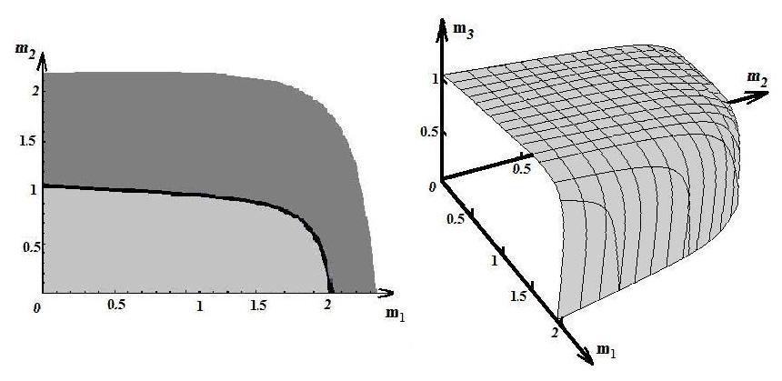
Figure 1: Examples of the criticality set $C$ for $N=2$ and $N=3$.

4 Moment analysis of CBP

It was Ch.J. Mode who showed (see [22]) that the mean particles numbers in a supercritical indecomposable multi-type Bellman-Harris process grow exponentially (as time tends to infinity) with a certain rate $\nu$ called a Malthusian parameter. The parameter $\nu$ is positive and determined as the unique solution to equation $\rho(H(\nu))=1$. Lemma 1 demonstrates that for our auxiliary $L$-dimensional supercritical Bellman-Harris process this procedure can be simplified and the Malthusian parameter can be found as the unique solution to equation $\rho(D(\nu))=1$ (observe that square matrix $H(\lambda)$ is of size $L\geq N$ whereas square matrix $D(\lambda)$ is of size $N$). So, in the framework of CBP the Malthusian parameter $\nu$ is defined as the unique (positive) solution to equation $\rho(D(\nu))=1$ whenever $\rho(D)>1$. Given $\rho(D)=\rho(D(0))>1$, such solution always exists, since according to the Perron-Frobenius theorem the function $\rho(D(\lambda))$ in variable $\lambda$ is strictly decreasing and tends to $0$ as $\lambda\to\infty$.

Recall that, for an $n\times n$ matrix $R$, the matrix $R_{i,j}$ or $(R)_{i,j}$ is the ${(n-1)\times(n-1)}$ matrix that results from deleting the $i$-th row and the $j$-th column of $R$, $i,j=1,\ldots,n$. To formulate our main result we need some new notation. For supercritical CBP consider functions $a_{n}(x,y)$, $x,y\!\in\!S$, $n\!\in\!\bf N$, which appear in description of the asymptotic behavior, as $t\to\infty$, of the $n$-th factorial moments ${m_{n}(t;x,y):={\sf E}_{x}\mu(t;y)(\mu(t;y)-1)\ldots(\mu(t;y)-n+1)}$ of the local particles numbers in CBP (index $x$ denotes the starting point of CBP). The function $a_{1}(x,y)$ has the most concise form when $x,y\in W$, namely,

$$a_{1}(w_{i},w_{j})=\frac{\Delta_{j,i}(\nu)}{(\nu+\beta_{j})\Delta^{\prime}(\nu)},\quad i,j=1,\ldots,N,$$ (8)

where $\Delta_{i,j}(\lambda)\!:=\!(-1)^{i+j}\det(I-D(\lambda))_{i,j}$ and $\Delta^{\prime}(\nu)\!:=\!\left.\frac{d}{d\lambda}\det(I-D(\lambda))\right|_{\lambda=\nu}$. If $N=1$ then $\Delta_{1,1}(\lambda)$, $\lambda\geq 0$, is supposed to be identically $1$. For $x\in W$ and $y\in S\setminus W$ we set

$$a_{1}(w_{i},y)=\frac{\sum_{j=1}^{N}\Delta_{j,i}(\nu)(1-\alpha_{j})G^{\ast}_{j}(\nu){{}_{W}\overline{F}^{\ast}_{w_{j},y}(\nu)}}{(\nu-q(y,y))\Delta^{\prime}(\nu)(1-{{}_{W}F^{\ast}_{y,y}(\nu)})},\quad i=1,\ldots,N.$$ (9)

Here ${{}_{H}F^{\ast}_{x^{\prime},y^{\prime}}(\lambda)}:=(-q(x^{\prime},x^{\prime}))(\lambda-q(x^{\prime},x^{\prime}))^{-1}{{}_{H}\overline{F}^{\ast}_{x^{\prime},y^{\prime}}(\lambda)}$, $\lambda\geq 0$, $x^{\prime},y^{\prime}\in S$, $H\subset S$, i.e. ${{}_{H}F_{x^{\prime},y^{\prime}}(t)}$, $t\geq 0$, is the c.d.f. of a hitting time of state $y^{\prime}$ under taboo $H$ given that the Markov chain $\eta$ starts at state $x^{\prime}$ (see, e.g., [9]). Note that $G^{\ast}_{j}(\lambda)=\beta_{j}(\lambda+\beta_{j})^{-1}$ for each $\lambda\geq 0$ and $j=1,\ldots,N$. The values $a_{n}(x,y)$ for $n>1$, $x\in W$ and $y\in S$ are evaluated with the help of the following iterative scheme

$$a_{n}(w_{i},y)=\sum\limits_{k=1}^{N}\frac{\beta_{k}\Delta_{k,i}(n\nu)}{(n\nu+\beta_{k})\Delta(n\nu)}h_{n,k}(a_{1}(w_{k},y),\ldots,a_{n-1}(w_{k},y))$$ (10)

where $i=1,\ldots,N$, $\Delta(\lambda):=\det(I-D(\lambda))$, $\lambda\geq 0$,

$$h_{n,k}(z_{1},\ldots,z_{n-1}):=\alpha_{k}\sum\limits_{r=2}^{n}\frac{f^{(r)}_{k}(1)}{r!}\sum\limits_{\begin{subarray}{c}i_{1},\ldots,i_{r}>0,\\ i_{1}+\ldots+i_{r}=n\end{subarray}}\frac{n!}{i_{1}!\ldots i_{r}!}z_{i_{1}}\ldots z_{i_{r}}$$ (11)

and $z_{1},\ldots,z_{n-1}\geq 0$, $k=1,\ldots,N$. In this way the values $a_{n}(x,y)$ for $n\geq 1$, $x\in S\setminus W$ and $y\in S$ are determined by formula

$$a_{n}(x,y)=\sum\nolimits_{i=1}^{N}{{}_{W_{i}}F^{\ast}_{x,w_{i}}(n\nu)}a_{n}(w_{i},y).$$ (12)

Define functions $A_{n}(x)$, $x\in S$, $n\in{\bf N}$, arising in the asymptotic behavior of the $n$-th factorial moments ${M_{n}(t;x):={\sf E}_{x}\mu(t)(\mu(t)-1)\ldots(\mu(t)-n+1)}$ of the total particles numbers in supercritical CBP. Namely, for $n=1$ and $x\in W$, put

$$A_{1}(w_{i})=\sum\limits_{j=1}^{N}\frac{\alpha_{j}\beta_{j}(f^{\prime}_{j}(1)-1)\Delta_{j,i}(\nu)}{\nu(\nu+\beta_{j})\Delta^{\prime}(\nu)},\quad i=1,\ldots,N.$$ (13)

When $n>1$ and $x\in W$ the values $A_{n}(x)$ are evaluated according to the following iterative scheme

$$A_{n}(w_{i})=\sum_{j=1}^{N}\frac{\beta_{j}\Delta_{j,i}(n\nu)}{(n\nu+\beta_{j})\Delta(n\nu)}h_{n,j}(A_{1}(w_{j}),\ldots,A_{n-1}(w_{j}))$$ (14)

where $i=1,\ldots,N$. Bearing on the latter equalities the values $A_{n}(x)$ for $n\geq 1$ and $x\in S\setminus W$ are obtained by way of

$$A_{n}(x)=\sum\nolimits_{i=1}^{N}{{}_{W_{i}}F^{\ast}_{x,w_{i}}(n\nu)}A_{n}(w_{i}).$$ (15)

For critical CBP introduce functions $b_{n}(x,y)$ and $B_{n}(x)$, $x,y\in S$, $n\in{\bf N}$, appearing in the asymptotic behavior of $m_{n}(t;x,y)$ and $M_{n}(t;x)$, respectively. Namely, for $i,j=1,\ldots,N$ and $y\in S\setminus W$, set

$$b_{1}(w_{i},w_{j})=\frac{\Delta_{j,i}(0)}{\beta_{j}\Delta^{\prime}(0)},\quad b_{1}(w_{i},y)=\frac{\sum_{j=1}^{N}\Delta_{j,i}(0)(1-\alpha_{j}){{}_{W}F_{w_{j},y}(\infty)}}{(-q(y,y))\Delta^{\prime}(0)(1-{{}_{W}F_{y,y}(\infty)})}$$ (16)

where $\Delta^{\prime}(0):=\left.\frac{d}{d\lambda}\det(I-D(\lambda))\right|_{\lambda=0+}$. When $n>1$, $i=1,\ldots,N$ and $y\in S$, the values $b_{n}(w_{i},y)$ are evaluated by the iterative scheme

$$b_{n}(w_{i},y)=\sum_{k=1}^{N}\frac{\alpha_{k}f^{\prime\prime}_{k}(1)\Delta_{k,i}(0)}{2(n-1)\Delta^{\prime}(0)}\sum_{r=1}^{n-1}\binom{n}{r}b_{r}(w_{k},y)b_{n-r}(w_{k},y).$$ (17)

Thus the values $b_{n}(x,y)$ for $n\geq 1$, $x\in S\setminus W$ and $y\in S$ are determined by the formula

$$b_{n}(x,y)=\sum\nolimits_{i=1}^{N}{{}_{W_{i}}F_{x,w_{i}}(\infty)}b_{n}(w_{i},y).$$ (18)

For $i=1,\ldots,N$ put

$$B_{1}(w_{i})=\sum_{j=1}^{N}\frac{\alpha_{j}(f^{\prime}_{j}(1)-1)\Delta_{j,i}(0)}{\Delta^{\prime}(0)}.$$ (19)

When $n>1$ the values $B_{n}(w_{i})$ are computed iteratively, namely,

$$B_{n}(w_{i})=\sum_{j=1}^{N}\frac{\alpha_{j}f^{\prime\prime}_{j}(1)\Delta_{j,i}(0)}{2(2n-1)\Delta^{\prime}(0)}\sum_{r=1}^{n-1}\binom{n}{r}B_{r}(w_{j})B_{n-r}(w_{j}),\;i=1,\ldots,N.$$ (20)

Bearing on the latter equalities the values $B_{n}(x)$ for $n\geq 1$ and $x\in S\setminus W$ are given as follows

$$B_{n}(x)=\sum\nolimits_{i=1}^{N}{{}_{W_{i}}F_{x,w_{i}}(\infty)}B_{n}(w_{i}).$$ (21)

At last, for subcritical CBP define functions $C_{n}(x)$, $x\in S$, $n\in{\bf N}$, arising in the description of the asymptotic behavior for $M_{n}(t;x)$. Set

$$C_{1}(w_{i})=1+\sum_{j=1}^{N}\frac{\alpha_{j}(f^{\prime}_{j}(1)-1)\Delta_{j,i}(0)}{\Delta(0)},\quad i=1,\ldots,N,$$ (22)

$$C_{1}(x)=1-\sum\nolimits_{i=1}^{N}{{}_{W_{i}}F_{x,w_{i}}(\infty)}+\sum\nolimits_{i=1}^{N}{{}_{W_{i}}F_{x,w_{i}}(\infty)C_{1}(w_{i})},\quad x\in S\setminus W,$$ (23)

and, for $n>1$, put

$$C_{n}(w_{i})=\sum_{j=1}^{N}\frac{\Delta_{j,i}(0)}{\Delta(0)}h_{n,j}(C_{1}(w_{j}),\ldots,C_{n-1}(w_{j})),\quad i=1,\ldots,N,$$ (24)

$$C_{n}(x)=\sum\nolimits_{i=1}^{N}{{}_{W_{i}}F_{x,w_{i}}(\infty)}C_{n}(w_{i}),\quad x\in S\setminus W.$$ (25)

The following theorem is the main result of Section 4 providing the moment analysis of the local and total particles numbers in CBP. This theorem generalizes Theorems 4.1, 4.2 in [34] and Theorem 1 in [14] as well as some statements of Theorem 2 in [2].

Theorem 1

For each $n\in{\bf N}$, given that ${\sf E}\xi^{n}_{i}<\infty$ for any $i=1,\ldots,N$, functions $m_{n}(t;x,y)$ and $M_{n}(t;x)$ are bounded on every finite interval in $[0,\infty)$ for fixed $x,y\in S$. Moreover, whenever ${\sf E}\xi^{n}_{i}<\infty$ for any $i=1,\ldots,N$, the asymptotic behavior of $m_{n}(t;x,y)$ and $M_{n}(t;x)$ as $t\to\infty$ depends essentially on the class of CBP and is as follows.

1. If $\rho(D)>1$ then $\nu>0$ and

   $$m_{n}(t;x,y) = a_{n}(x,y)e^{n\nu t}+o\left(e^{n\nu t}\right),$$ (26)

   $$M_{n}(t;x) = A_{n}(x)e^{n\nu t}+o\left(e^{n\nu t}\right),\quad t\to\infty,$$ (27)

   where functions $a_{n}(x,y)$ and $A_{n}(x)$, $x,y\in S$, are strictly positive.

2. If $\rho(D)=1$ then

   $$m_{n}(t;x,y) = b_{n}(x,y)t^{n-1}+o\left(t^{n-1}\right),$$ (28)

   $$M_{n}(t;x) = B_{n}(x)t^{2n-1}+o\left(t^{2n-1}\right),\quad t\to\infty,$$ (29)

   where function $b_{n}(x,y)$ is strictly positive for any values $x,y\in S$ iff ${\int_{0}^{\infty}u\,d{{}_{W_{j}}\overline{F}_{w_{i},w_{j}}(u)}<\infty}$ for each $i,j=1,\ldots,N$ and, in addition, in case of recurrent $\eta$ and $n\geq 2$ one has $\sum\nolimits_{i=1}^{N}\alpha_{i}\left|f_{i}(s)-s\right|>0$ for some $s\in[0,1)$. Moreover, $B_{n}(x)$ is strictly positive for any $x\in S$ iff the Markov chain $\eta$ is transient and $\int_{0}^{\infty}u\,d{{}_{W_{j}}\overline{F}_{w_{i},w_{j}}(u)}<\infty$ for each $i,j=1,\ldots,N$. Otherwise, respectively ${b_{n}(\cdot,\cdot)\equiv 0}$ and $B_{n}(\cdot)\equiv 0$.

3. If $\rho(D)<1$ then

   $$m_{n}(t;x,y) = o(1),$$ (30)

   $$M_{n}(t;x) = C_{n}(x)+o(1),\quad t\to\infty,$$ (31)

   where function $C_{n}(x)$ is strictly positive for each $x\in S$ iff the Markov chain $\eta$ is transient. Otherwise, $C_{n}(\cdot)\equiv 0$.

Stress that we do not impose any restrictions on the character of the Markov chain $\eta$ such as symmetry and homogeneity of transition probabilities or finite variance of jump sizes etc. Therefore, in Theorem 1 we establish exact asymptotic relations in item 1 and only partially in items 2 and 3. It is not possible to give any useful and general information on items 2 and 3 without further knowledge of the underlying motion. For instance, even for critical symmetric branching random walk on ${\bf Z}^{d}$ with a single catalyst (see [2]) there are four different asymptotic formulae for $m_{n}(t;x,y)$ and $M_{n}(t;x)$ depending on dimension $d=1,2,3$ or $4$ and thereby on the decay rate of transition probabilities (note that for $d\geq 5$ Theorem 1 generalizes the corresponding results in [2]). Moreover, for subcritical branching random walk on ${\bf Z}^{d}$ with a single catalyst (see [7]) the decay orders of $m_{n}(t;x,y)$ do not coincide for different $d\in{\bf N}$.

Let us proceed to the proof of Theorem 1.

Proof. We will mainly employ the auxiliary Bellman-Harris process constructed in Section 2. Firstly we establish Theorem 1 for $x,y\in W$ (Case 1) and afterwards extend these results to the general case $x,y\in S$ (Case 2).

Case 1. So, assume that $x,y\in W$. The following proof of Theorem 1 for Case 1 is divided into $9$ steps. At step 1 we derive a system of renewal equations involving the factorial moments of the local particles numbers in CBP. Then at steps 2, 3 and 4 we employ this system to prove the corresponding assertions (26), (28) and (30) of Theorem 1 related to moment analysis of the local particles numbers. Next at steps 5 and 6 we derive a system of renewal equations involving the factorial moments of the total particles number in CBP depending on whether the Markov chain $\eta$ is recurrent or transient. At last, at steps 7, 8 and 9 we exploit these systems to establish statements (27), (29) and (31) of Theorem 1, respectively, concerning the moment analysis of the total particles number. Note that at step 6 we introduce an auxiliary decomposable $(L+1)$-dimensional Bellman-Harris process with a final type of particles.

Step 1. At this stage we derive a system of renewal equations involving the factorial moments of local particles numbers in CBP. Denote by $m^{BH}_{n}(t;k,l):={\bf E}_{k}Z_{l}(t)(Z_{l}(t)-1)\ldots(Z_{l}(t)-n+1)$, for $t\geq 0$, $n\in{\bf N}$ and ${k,l=1,\ldots,L}$, the $n$-th factorial moment of the number of particles $Z_{l}(t)$ of the $l$-th type at time $t$ in the Bellman-Harris process (index $k$ stands for the type of the parent particle). According to the construction of the auxiliary process one has $m_{n}(t;w_{i},w_{j})=m^{BH}_{n}(t;i,j)$ for each $n\in{\bf N}$, $t\geq 0$, $i,j=1,\ldots,N$. Thus, given that ${\bf E}\xi^{n}_{k}<\infty$ for some $n\in{\bf N}$ and any $k=1,\ldots,N$, the finiteness of functions $m_{n}(t;w_{i},w_{j})$ for each $t\geq 0$ and $i,j=1,\ldots,N$, follows from Theorem 1 in [27], Ch.8, Sec.6. Moreover, in view of this theorem functions $m^{BH}_{1}(t;k,l)$, $t\geq 0$, $k,l=1,\ldots,L$, satisfy the following system of renewal equations

$$m^{BH}_{1}(t;k,l)=\delta_{k,l}(1-G_{k}(t))+\sum\limits_{r=1}^{L}m_{k,r}\int\nolimits_{0}^{t}m^{BH}_{1}(t-u;r,l)\,dG_{k}(u)$$ (32)

while for $n>1$ this theorem and the generalized Faá di Bruno’s formula (see [20]) entail

$$m^{BH}_{n}(t;k,l)=\sum_{r=1}^{L}m_{k,r}\int\nolimits_{0}^{t}{m^{BH}_{n}(t-u;r,l)\,dG_{k}(u)}$$

$$+ \sum^{\sim}\frac{n!}{\prod\nolimits_{p=1}^{n-1}i^{(1)}_{p}!\ldots i^{(L)}_{p}!}\left.\frac{\partial^{J(1)+\ldots+J(L)}g_{k}({\bf s})}{\partial s_{1}^{J(1)}\ldots\partial s_{L}^{J(L)}}\right|_{{\bf s}=(1,\ldots,1)}$$

$$\times \int\nolimits_{0}^{t}\prod_{p=1}^{n-1}\left(\left(\frac{m^{BH}_{p}(t-u;1,l)}{p!}\right)^{i^{(1)}_{p}}\ldots\left(\frac{m^{BH}_{p}(t-u;L,l)}{p!}\right)^{i^{(L)}_{p}}\right)\,dG_{k}(u).$$

Here the symbol $\sum\limits^{\sim}$ means the sum taken over all $L$-dimensional vectors ${{\bf i}_{1}=\left(i^{(1)}_{1},\ldots,i^{(L)}_{1}\right)}$, $\ldots$, ${\bf i}_{n-1}=\left(i^{(1)}_{n-1},\ldots,i^{(L)}_{n-1}\right)$ with nonnegative integer components satisfying the following equality $\sum\nolimits_{p=1}^{n-1}p\left(i^{(1)}_{p}+\ldots+i^{(L)}_{p}\right)=n$. For every ${r=1,\ldots,L}$, we also put ${J(r):=\sum\nolimits_{p=1}^{n-1}i^{(r)}_{p}}$. Substituting the explicit formulae (1) and (2) for the offspring generating functions $g_{k}(\cdot)$, $k=1,\ldots,L$, of the Bellman-Harris process in (4) we come to more concise relation

$$m^{BH}_{n}(t;k,l)=\sum_{r=1}^{L}m_{k,r}\int\nolimits_{0}^{t}{m^{BH}_{n}(t-u;r,l)\,dG_{k}(u)}$$

$$+ {\bf I}(k\in\{1,\ldots,N\})\sum\limits^{\approx}\frac{\alpha_{k}f^{(J)}_{k}(1)\,n!}{i_{1}!\ldots i_{n-1}!}\int\nolimits_{0}^{t}\prod_{p=1}^{n-1}\left(\frac{m^{BH}_{p}(t-u;k,l)}{p!}\right)^{i_{p}}\!\!\!dG_{k}(u)$$

where ${\bf I}(\cdot)$ is the indicator and the symbol $\sum\limits^{\approx}$ means the sum taken over all nonnegative integer $i_{1}$, $\ldots$, $i_{n-1}$ such that $\sum\nolimits_{p=1}^{n-1}p\,i_{p}=n$. We also use the notation $J:=i_{1}+\ldots+i_{n-1}$.

Step 2. Now we prove the part of assertion (26) related to the case $x,y\in W$. So, assume that $\rho(D)>1$. Applying Theorem 2.1, item (iii), in [12] to the system of renewal equations (32) we get

$$e^{-\nu t}\,m^{BH}_{1}(t;i,j)\to\frac{(-1)^{i+j}\det(I-H(\nu))_{j,i}}{(\nu+\beta_{j})\left.\frac{d}{d\lambda}\det(I-H(\lambda))\right|_{\lambda=\nu}},\quad t\to\infty,$$ (35)

for each $i,j=1,\ldots,N$. Here $\nu>0$ and $\left.\frac{d}{d\lambda}\det(I-H(\lambda))\right|_{\lambda=\nu}>0$ (see, e.g., [22]). Comparing formulae (8) and (26) with (35) we see that one needs to establish relations between determinants and algebraic adjuncts of matrices $I-H(\lambda)$ and $I-D(\lambda)$. The following lemma provides them.

Lemma 2

For each $\lambda\geq 0$ and $i=1,\ldots,|K_{j}|$, $j,k=1,\ldots,N$, one has

$$\det(I-H(\lambda))=\det(I-D(\lambda)),\quad\det(I-H(\lambda))_{j,k}=\det(I-D(\lambda))_{j,k},$$

$$(-1)^{L(j)+i+k}\det(I-H(\lambda))_{L(j)+i,k}=(-1)^{j+k}m_{j,L(j)+i}G^{\ast}_{j}(\lambda)\det(I-D(\lambda))_{j,k}.$$

Proof. We apply transformations to the columns of matrix $I-H(\lambda)$ which do not change its determinant. Namely, for each ${j,k=1,\ldots,N}$ add the $(L(j)+i)$-th column multiplied by $G^{\ast}_{L(j)+i}(\lambda)$ to the $k$-th column if $k\in K_{j}$, i.e. $k=k(i,j)$ for some $i=1,\ldots,|K_{j}|$. After these transformations we get a block matrix consisting of four blocks. The left upper block of size $N\times N$ is just $I-D(\lambda)$ whereas the left lower $(L-N)\times N$ and the right lower $(L-N)\times(L-N)$ blocks are the zero and the identity matrices, respectively. Employing the formula for the determinant of a block matrix (see, e.g., [19], vol.1, Ch.2, Sec.5) we come to the first assertion of Lemma 2. The second one is established in the same manner. To prove the third assertion we apply the above transformations to the matrix $(I-H(\lambda))_{L(j)+i,k}$ and then shift the column number $L(j)+i-1$ to the column number $N$. The determinants of the matrix $(I-H(\lambda))_{L(j)+i,k}$ and the transformed one are equal up to the factor $(-1)^{L(j)+i-N-1}$. Afterwards, we involve the formula for the determinant of a block matrix once again and use the Laplace expansion of determinants with respect to the $N$-th column. Lemma 2 is proved completely. $\square$

Thus, by virtue of (35) and Lemma 2 we prove (26) when $n=1$ and ${x,y\in W}$. Before focusing on the case $n\!>\!1$ let us note that in [22] Ch.J. Mode found the asymptotic behavior of the mean particles numbers in supercritical multi-type Bellman-Harris process under rather restrictive conditions that each c.d.f. $G_{k}(\cdot)$ has a square-integrable density. This is the reason why we bear on similar results by K. Crump established in [12] without any additional assumptions and not on the mentioned results by Ch.J. Mode. To check relation (26) when $n>1$ and $x,y\in W$ we employ the induction method in variable $n$. The case $n=1$ is verified above. Let formula (26) be valid for all the moment orders not exceeding $n-1$. Then the second term at the right-hand side of (4) denoted by $V_{n}(t;k,l)$ has the following asymptotic behavior

$$V_{n}(t;k,l)\!\sim\!{\bf I}(k\in\{1,\ldots,N\})e^{n\nu t}G^{\ast}_{k}(n\nu)\sum\limits^{\approx}\frac{\alpha_{k}f^{(J)}_{k}(1)\,n!}{i_{1}!\ldots i_{n-1}!}\prod_{p=1}^{n-1}\!\!\left(\frac{a_{p}(w_{k},w_{l})}{p!}\right)^{i_{p}}$$

as $t\to\infty$, for each $k=1,\ldots,L$ and $l=1,\ldots,N$. Taking into account the latter relation and applying Theorem 2.1, item (iv), in [12] to the system of renewal equations (4) we obtain

$$\frac{m^{BH}_{n}\!(t;i,j)}{e^{n\nu t}}\!\to\!\!\sum\limits_{k=1}^{N}\!\!\frac{(\!-\!1)^{i+k}\beta_{k}\det(I\!-\!H(n\nu))_{k,i}}{(n\nu+\beta_{k})\det(I\!-\!H(n\nu))}h_{n,k}(a_{1}\!(w_{k},w_{j}),\!...,a_{n-\!1}\!(w_{k},w_{j}))$$

as $t\to\infty$, for each $i,j=1,\ldots,N$. Here we use the alternative representation (see, e.g., [1], Theorem 3.3) for function $h_{n,k}$ defined in (11). The latter asymptotic relation combined with Lemma 2 and formula (10) leads to the desired statement in (26) when $n>1$ and $x,y\in W$. Note that functions $a_{n}(w_{i},w_{j})$, $n\geq 1$, $i,j=1,\ldots,N$, are strictly positive according to, e.g., [19], vol.2, Ch.13, Sec.3.

Step 3. Next we prove assertion (28) for $x,y\in W$. Assume that $\rho(D)=1$ or, equivalently, that the unique solution to $\rho(D(\nu))=1$ is $\nu=0$. Applying Theorem 2.1, item (iii), in [12] to (32) we come to the following relation

$$m^{BH}_{1}(t;i,j)\to\frac{(-1)^{i+j}\det(I-H(0))_{j,i}}{\beta_{j}\left.\frac{d}{d\lambda}\det(I-H(\lambda))\right|_{\lambda=0+}},\quad t\to\infty,\quad i,j=1,\ldots,N.$$

This formula along with (16) and Lemma 2 entail the required statement of (28) when $n=1$. For $n>1$ we employ the induction method in variable $n$. Performing the induction step we get

$$V_{n}(t;k,l) \sim \sum\limits^{\approx}\frac{\alpha_{k}f^{(J)}_{k}(1)\,n!}{i_{1}!\ldots i_{n-1}!}\prod_{p=1}^{n-1}\left(\frac{b_{p}(w_{k},w_{l})}{p!}\right)^{i_{p}}\int\nolimits_{0}^{t}(t-u)^{n-J}dG_{k}(u)$$

$$\sim t^{n-2}\,\frac{\alpha_{k}f^{\prime\prime}_{k}(1)}{2}\sum_{r=1}^{n-1}\binom{n}{r}b_{r}(w_{k},w_{l})b_{n-r}(w_{k},w_{l}),\quad t\to\infty,$$

for $k,l=1,\ldots,N$, whereas $V_{n}(t;k,l)=0$, for $k=N+1,\ldots,L$, $l=1,\ldots,N$. Hence, applying Theorem 2.1, item (v), in [12] to (4) we see that

$$\frac{m^{BH}_{n}\!(t;i,j)}{t^{n-1}}\!\to\!\!\sum_{k=1}^{N}\!\!\frac{(\!-\!1)^{i+k}\!\alpha_{k}f^{\prime\prime}_{k}(1)\!\det(I\!-\!H(0))_{k,i}}{2(n\!-\!1)\!\!\left.\frac{d}{d\lambda}\det(I\!-\!H(\lambda))\right|_{\lambda=0+}}\!\sum_{r=1}^{n-1}\!\!\binom{\!n\!}{r}b_{r}\!(w_{k},\!w_{j})b_{n\!-r}\!(w_{k},\!w_{j})$$

as $t\to\infty$, for each $i,j=1,\ldots,N$. The assertion (28) for $n>1$ now follows from the latter relation, definition (17) and Lemma 2. In view of [19], vol.2, Ch.13, Sec.3, the algebraic adjunct $\Delta_{i,j}(0)$ is strictly positive for any $i,j=1,\ldots,N$. As was established in [22] one has $\Delta^{\prime}(0)\in(0,\infty]$. Moreover, $\Delta^{\prime}(0)<\infty$ iff $\int\nolimits_{0}^{\infty}u\,d{{}_{W_{j}}\overline{F}_{w_{i},w_{j}}(u)}<\infty$ for each $i,j=1,\ldots,N$. Therefore, functions $b_{n}(w_{i},w_{j})$ are strictly positive for any $n\in{\bf N}$, $i,j=1,\ldots,N$ if and only if $\int\nolimits_{0}^{\infty}u\,d{{}_{W_{j}}\overline{F}_{w_{i},w_{j}}(u)}<\infty$ and, in addition, in case of recurrent $\eta$ and $n\geq 2$ one has $\sum\nolimits_{i=1}^{N}\alpha_{i}\left|f_{i}(s)-s\right|>0$ for some $s\in[0,1)$. Note that the latter condition allows us to separate the case of ordinary motion of particles without breeding. Such CBP is critical for recurrent Markov chain $\eta$ and subcritical for transient $\eta$.

Step 4. Relation (30) for the case $x,y\in W$ is verified by application of Theorem 2.2, item (ii), in [23] to (32) and (4). Here we essentially bear on the fact that $M^{n}$ converges elementwise to the zero matrix, as $n\to\infty$, since in subcritical case $\rho(M)<1$ on account of Lemma 1.

Step 5. Let us derive a system of renewal equations involving the factorial moments of the total particles number when $x\in W$ and $\eta$ is recurrent. Denote by $Z(t):=\sum_{j=1}^{L}Z_{j}(t)$, $t\geq 0$, the total particles number at time $t$ in the auxiliary Bellman-Harris process. According to the construction of this process the distribution laws of $\mu(t)$ and $Z(t)$ are the same for each $t\geq 0$ iff the Markov chain $\eta$ is recurrent. Indeed, whenever the Markov chain $\eta$ is transient, with positive probability there are particles at time $t$ in CBP having infinite life-lengths since they will never hit the set $W$ after time $t$. These particles are not comprised by our $L$-dimensional Bellman-Harris process. So, we will now concentrate on the recurrent case. Then one has $M_{n}(t;w_{i})=M^{BH}_{n}(t;i)$ for each $t\geq 0$, $n\in{\bf N}$ and $i=1,\ldots,N$ where $M^{BH}_{n}(t;k):={\bf E}_{k}Z(t)(Z(t)-1)\ldots(Z(t)-n+1)$, $t\geq 0$, $n\in{\bf N}$ and ${k=1,\ldots,L}$. Thus, given that ${\bf E}\xi^{n}_{l}<\infty$ for some $n\in{\bf N}$ and any ${l=1,\ldots,N}$, Theorem 1 in [27], Ch.8, Sec.6, implies the finiteness of functions $M_{n}(t;w_{i})$ for each $t\geq 0$ and $i=1,\ldots,N$. Moreover, in view of this theorem functions $M^{BH}_{1}(t;k)$, $t\geq 0$, $k=1,\ldots,L$, satisfy the following system of renewal equations

$$M^{BH}_{1}(t;k)=1-G_{k}(t)+\sum\limits_{r=1}^{L}m_{k,r}\int\nolimits_{0}^{t}M^{BH}_{1}(t-u;r)\,dG_{k}(u).$$ (36)

For $n>1$ this theorem and the generalized Faá di Bruno’s formula (see [20]) entail equations in $M^{BH}_{n}(t;k)$ the same as those obtained from (4) after replacing $m^{BH}_{n}(t;k,l)$ by $M^{BH}_{n}(t;k)$. Therefore, for $M^{BH}_{n}(t;k)$, $t\geq 0$, $k=1,\ldots,L$, the system of renewal equations (4) holds true if function $m^{BH}_{n}(t;k,l)$ is replaced by $M^{BH}_{n}(t;k)$.

Step 6. Next consider CBP with the underlying motion of particles governed by transient Markov chain $\eta$. To cover the transient case we construct a new auxiliary Bellman-Harris process with particles of $L+1$ types such that the $(L+1)$-th type is final (see, e.g., [27], Ch.5, Sec.3, and [29]). For the new Bellman-Harris process, the c.d.f. of the life-length of a particle of $j$-th type is denoted by $\widehat{G}_{j}(t)$, $t\geq 0$, whereas its offspring generating function is $\widehat{g}_{j}({\bf s},s_{L+1})$, ${{\bf s}\in[0,1]^{L}}$, $s_{L+1}\in[0,1]$, $j=1,\ldots,L+1$. Let $\widehat{G}_{i}(t)=G_{i}(t)$, $t\geq 0$, for $i=1,\ldots,L$, and $\widehat{g}_{j}({\bf s},s_{L+1})=g_{j}({\bf s})$, ${\bf s}\in[0,1]^{L}$, $s_{L+1}\in[0,1]$, for $j=N+1,\ldots,L$, where $G_{i}$ and $g_{j}$ are defined in (1) and (2). Then put

$$\widehat{g}_{j}({\bf s},s_{L+1})=\alpha_{j}f_{j}(s_{j})+(1-\alpha_{j})\sum\limits_{k=1}^{N}{{}_{W_{k}}\overline{F}_{w_{j},w_{k}}(0)s_{k}}$$

$$+(1-\alpha_{j})\sum\limits_{i=1}^{|K_{j}|}{T_{i,j}(\infty)s_{L(j)+i}}+(1-\alpha_{j})\left(1-\sum\limits_{k=1}^{N}{{}_{W_{k}}\overline{F}_{w_{j},w_{k}}(\infty)}\right)s_{L+1},$$

for $j=1,\ldots,N$, ${\bf s}\in[0,1]^{L}$, $s_{L+1}\in[0,1]$, i.e. definitions of functions $g_{j}$ and $\widehat{g}_{j}$ differ by the last term only. Since the $(L+1)$-th type is final, that is every particle of the $(L+1)$-th type has infinite life-length and does not produce any offsprings, for the sake of definiteness we may set ${\widehat{G}_{L+1}(t)=0}$, $t\geq 0$, and $\widehat{g}_{L+1}({\bf s},s_{L+1})=s_{L+1}$, ${\bf s}\in[0,1]^{L}$, ${s_{L+1}\in[0,1]}$. The mean matrix $\widehat{M}=(\widehat{m}_{k,l})_{k,l=1}^{L+1}$ of the new process has entries ${\widehat{m}_{k,l}=m_{k,l}}$, for $k,l=1,\ldots,L$, $\widehat{m}_{i,L+1}=(1-\alpha_{i})\left(1-\sum\nolimits_{k=1}^{N}{{}_{W_{k}}\overline{F}_{w_{i},w_{k}}(\infty)}\right)$, $i=1,\ldots,N$, $\widehat{m}_{L+1,L+1}=1$ and $\widehat{m}_{k,l}=0$ for the remaining pairs of $k$ and $l$. Let $\widehat{Z}_{j}(t)$, $t\geq 0$, ${j=1,\ldots,L+1}$, be the number of particles of type $j$ at time $t$ in the new Bellman-Harris process. Evidently, the distributions of vectors $(\widehat{Z}_{1}(t),\ldots,\widehat{Z}_{L}(t))$ and $(Z_{1}(t),\ldots,Z_{L}(t))$ coincide for each $t\geq 0$ whenever the parent particles of both Bellman-Harris processes have the same type. Moreover, the new process takes into account even the particles from the ${(L+1)}$-th group of particles in CBP (see Section 2) which are not comprised by the $L$-dimensional Bellman-Harris process. Thus, for each $n\in{\bf N}$, ${i=1,\ldots,N}$ and $t\geq 0$, one has $M_{n}(t;w_{i})=\widehat{M}^{BH}_{n}(t;i)$ where we write ${\widehat{M}^{BH}_{n}(t;k):={\bf E}_{k}\widehat{Z}(t)(\widehat{Z}(t)-1)\ldots(\widehat{Z}(t)-n+1)}$, $k=1,\ldots,L+1$, and set ${\widehat{Z}(t):=\sum_{j=1}^{L+1}\widehat{Z}_{j}(t)}$. Then applying Theorem 1 in [27], Ch.8, Sec.6, we ascertain that whenever ${\bf E}\xi^{n}_{l}<\infty$ for some $n\in{\bf N}$ and any $l=1,\ldots,N$, functions $M_{n}(t;w_{i})$ are finite for each $t\geq 0$ and $i=1,\ldots,N$. This theorem also implies that functions $\widehat{M}^{BH}_{1}(t;k)$, $t\geq 0$, $k=1,\ldots,L+1$, satisfy the following system of $L+1$ renewal equations

$$\widehat{M}^{BH}_{1}(t;k)=1-\widehat{G}_{k}(t)+\sum\limits_{r=1}^{L+1}\widehat{m}_{k,r}\int\nolimits_{0}^{t}\widehat{M}^{BH}_{1}(t-u;r)\,d\widehat{G}_{k}(u).$$

The $(L+1)$-th equation is just $\widehat{M}^{BH}_{1}(t;L+1)=1$, $t\geq 0$. Substituting that value $1$ and expressions for $\widehat{m}_{k,r}$, $r=1,\ldots,L+1$, into the first $L$ equations we get a new system of $L$ renewal equations

$$\!\!\widehat{M}^{BH}_{1}(t;k)=\sum\limits_{r=1}^{L}m_{k,r}\int\nolimits_{0}^{t}\widehat{M}^{BH}_{1}(t-u;r)\,dG_{k}(u)$$

$$+\!\! \!\!1-G_{k}(t)+{\bf I}\left(k\in\{1,\ldots,N\}\right)(1-\alpha_{k})\left(1-\sum\limits_{j=1}^{N}{{}_{W_{j}}\overline{F}_{w_{k},w_{j}}(\infty)}\right)G_{k}(t)$$

for $t\geq 0$ and $k=1,\ldots,L$. It is not difficult to verify that in view of Theorem 1 in [27], Ch.8, Sec.6, the system of $L+1$ equations resulting from (4) upon replacement of $L$ by $L+1$ and of $m^{BH}_{n}(t;k,l)$ by $\widehat{M}^{BH}_{n}(t;k)$ holds true for $n>1$, $t\geq 0$ and $k=1,\ldots,L+1$. The $(L+1)$-th equation is just $\widehat{M}^{BH}_{n}(t;L+1)=0$. Substituting that in the first $L$ equations and simplifying them similar to derivation of (4) we get the system of $L$ renewal equations in functions $\widehat{M}^{BH}_{n}(t;k)$, for $n>1$, $t\geq 0$ and $k=1,\ldots,L$, analogous to (4) but with $m^{BH}_{n}(t;k,l)$ replaced by $\widehat{M}^{BH}_{n}(t;k)$.

Step 7. Now we prove assertion (27) for the case $x,y\in W$. So, assume that $\rho(D)>1$. At first consider the recurrent case. Applying Theorem 2.1, item (iii), in [12] to (36) we see that

$$\frac{M^{BH}_{1}(t;i)}{e^{\nu t}}\!\to\!\!\sum_{j=1}^{N}\!\frac{\Delta_{j,i}(\nu)}{\nu\Delta^{\prime}(\nu)}\!\!\left(\!1-\alpha_{j}G^{\ast}_{j}(\nu)-(1-\alpha_{j})G^{\ast}_{j}(\nu)\!\!\sum_{k=1}^{N}\!{{}_{W_{k}}\overline{F}^{\ast}_{w_{j},w_{k}}(\nu)}\!\!\right)$$

$$= \sum_{k=1}^{N}\sum_{j=1}^{N}\frac{\Delta_{j,i}(\nu)}{\nu\Delta^{\prime}(\nu)}\left(\delta_{j,k}-\delta_{j,k}\alpha_{j}f^{\prime}_{j}(1)G^{\ast}_{j}(\nu)-(1-\alpha_{j})G^{\ast}_{j}(\nu){{}_{W_{k}}\overline{F}^{\ast}_{w_{j},w_{k}}(\nu)}\right)$$

$$+ \sum_{j=1}^{N}\frac{\alpha_{j}(f^{\prime}_{j}(1)-1)G^{\ast}_{j}(\nu)\Delta_{j,i}(\nu)}{\nu\Delta^{\prime}(\nu)}=\sum_{j=1}^{N}\frac{\alpha_{j}\beta_{j}(f^{\prime}_{j}(1)-1)\Delta_{j,i}(\nu)}{\nu(\nu+\beta_{j})\Delta^{\prime}(\nu)}$$

as $t\to\infty$ and $i=1,\ldots,N$. Here we rely on Lemma 2 and formulae (1)-(3) as well as on the Laplace expansion of determinants and obvious equality ${\sum_{k=1}^{N}{{}_{W_{k}}\overline{F}_{w_{j},w_{k}}(\infty)}=1}$ valid in the recurrent case. We also take into account that $\Delta(\nu)=0$ since $1$ is an eigenvalue of matrix $D(\nu)$. Relation (4) along with (13) lead to the desired statement (27) when $n=1$ and the Markov chain $\eta$ is recurrent. The transient case is treated in the same way except for two differences. The first one consists in employment of equations system (4) instead of (36). The second one is that for transient Markov chain $\eta$ the strict inequality ${\sum_{k=1}^{N}{{}_{W_{k}}\overline{F}_{w_{j},w_{k}}(\infty)}<1}$ holds true at least for some $j\in\{1,\ldots,N\}$. However, when deriving relation for $\widehat{M}^{BH}_{1}(t;i)$ similar to (4), the gap between the latter sum and $1$ is compensated by means of the additional summand in (4). Thus, when $n=1$ assertion (27) is established and the asymptotic behavior of $M_{1}(t;w_{i})$, $i=1,\ldots,N$, in supercritical CBP does not depend on whether the Markov chain $\eta$ is recurrent or transient. Since for $n>1$ the systems of equations in $M^{BH}_{n}(t;k)$ and $\widehat{M}^{BH}_{n}(t;k)$ respectively are of the same type as (4), the asymptotic behavior of $M_{n}(t;w_{i})$ in supercritical CBP is also independent of recurrence or transience of $\eta$. Moreover, when $n>1$ derivation of (27) for the total particles number almost literally repeats that of (30) for the local particles numbers and thus is omitted. Note that function $A_{1}(w_{i})$ (and, consequently, $A_{n}(w_{i})$ for $n>1$) is strictly positive for each $i=1,\ldots,N$ in view of positivity of the terms at the right-hand side of (4).

Step 8. Next proceed to the proof of statement (29) for the case $x,y\in W$. So, consider the case $\rho(D)=1$. Applying Theorem 2.1, item (v), in [12] to (4) we get

$$t^{-1}\widehat{M}^{BH}_{1}(t;i)\to\sum_{j=1}^{N}\frac{(1-\alpha_{j})\Delta_{j,i}(0)}{\Delta^{\prime}(0)}\left(1-\sum_{k=1}^{N}{{}_{W_{k}}\overline{F}_{w_{j},w_{k}}(\infty)}\right)$$

$$= \sum_{k=1}^{N}\sum_{j=1}^{N}\frac{\Delta_{j,i}(0)}{\Delta^{\prime}(0)}\left(\delta_{j,k}-\delta_{j,k}\,\alpha_{j}f^{\prime}_{j}(1)-(1-\alpha_{j}){{}_{W_{k}}\overline{F}_{w_{j},w_{k}}(\infty)}\right)$$

$$+ \sum_{j=1}^{N}\frac{\alpha_{j}(f^{\prime}_{j}(1)-1)\Delta_{j,i}(0)}{\Delta^{\prime}(0)}=\sum_{j=1}^{N}\frac{\alpha_{j}(f^{\prime}_{j}(1)-1)\Delta_{j,i}(0)}{\Delta^{\prime}(0)},\quad t\to\infty,$$

for $i=1,\ldots,N$. Here we use Lemma 2 as well as the Laplace expansion of determinants and equality $\Delta(0)=0$ valid by virtue of assumption ${\rho(D)=1}$. Relation (4) combined with (19) implies the desired assertion in (29) when $n=1$ and Markov chain $\eta$ is transient. When Markov chain $\eta$ is recurrent, the corresponding assertion follows from Theorem 2.1, item (i), in [12] and observation that the non-integral term at the right-hand side in (36) tends to $0$, as $t\to\infty$, whereas that in (4) converges to a positive limit at least for some $k\in\{1,\ldots,N\}$. For $n>1$ derivation of (29) for the total particles number again reproduces that of (28) for the local particles numbers and so is omitted. Note that in view of (4) function $B_{1}(w_{i})$ (and, consequently, $B_{n}(w_{i})$ for $n>1$) is strictly positive for each $i=1,\ldots,N$ iff $\Delta^{\prime}(0)<\infty$ and $\sum_{k=1}^{N}{{}_{W_{k}}\overline{F}_{w_{j},w_{k}}(\infty)}<1$ at least for some $j\in\{1,\ldots,N\}$.

Step 9. At last, let us establish (31) for the case $x,y\in W$. Thus, assume that $\rho(D)<1$. Applying Theorem 2.2, item (ii), in [23] to (4), we see that

$$\widehat{M}^{BH}_{1}(t;i)\to\sum_{j=1}^{N}\frac{(1-\alpha_{j})\Delta_{j,i}(0)}{\Delta(0)}\left(1-\sum_{k=1}^{N}{{}_{W_{k}}\overline{F}_{w_{j},w_{k}}(\infty)}\right)$$

$$= \sum_{k=1}^{N}\sum_{j=1}^{N}\frac{\Delta_{j,i}(0)}{\Delta(0)}\left(\delta_{j,k}-\delta_{j,k}\,\alpha_{j}f^{\prime}_{j}(1)-(1-\alpha_{j}){{}_{W_{k}}\overline{F}_{w_{j},w_{k}}(\infty)}\right)$$

$$+ \sum_{j=1}^{N}\frac{\alpha_{j}(f^{\prime}_{j}(1)-1)\Delta_{j,i}(0)}{\Delta(0)}=1+\sum_{j=1}^{N}\frac{\alpha_{j}(f^{\prime}_{j}(1)-1)\Delta_{j,i}(0)}{\Delta(0)},\quad t\to\infty,$$

for each $i=1,\ldots,N$. Here we involve Lemma 2 as well as the Laplace expansion of determinants and inequality $\Delta(0)>0$ valid on account of assumption $\rho(D)<1$. Formulae (22) and (4) entail the desired statement (31) when $n=1$ and Markov chain $\eta$ is transient. When Markov chain $\eta$ is recurrent, the corresponding relation ensues from (36) and Theorem 2.2, item (ii), in [23]. When $n>1$, this theorem also implies (31) due to equations system (4). Observe that in view of (4) function $C_{1}(w_{i})$ (and, consequently, $C_{n}(w_{i})$ for $n>1$) is strictly positive for each $i=1,\ldots,N$ iff $\sum_{k=1}^{N}{{}_{W_{k}}\overline{F}_{w_{j},w_{k}}(\infty)}<1$ for at least some $j\in\{1,\dots,N\}$, i.e. Markov chain $\eta$ is transient.

Thus, Theorem 1 is proved completely for the case $x,y\in W$.

Case 2. Now we assume that either $x\in S\setminus W$ or $y\in S\setminus W$ or ${x,y\in S\setminus W}$. The main idea of the rest of the proof is as follows. If $x\in S\setminus W$ and $y\in W$ we supplement the set of catalysts $W$ with $x$. Vice versa, if $x\in W$ and $y\in S\setminus W$ let us enlarge the set of catalysts $W$ by $y$. If ${x\in S\setminus W}$ and $y=x$ then we will add $x$ to the set of catalysts $W$. If both $x$ and $y$ are from $S\setminus W$ and, moreover, $x\neq y$, we supplement the set of catalysts $W$ with both states $x$ and $y$. Afterwards we may employ the already established results for CBP with $N+1$ or $N+2$ catalysts. So, set $w_{N+1}=x$, ${W(x):=W\cup\{x\}}$ and ${W_{i}(x):=W(x)\setminus\{w_{i}\}}$, ${i=1,\ldots,N+1}$. Let ${D(x;\lambda)=(d_{i,j}(x;\lambda))_{i,j=1}^{N+1}}$ be matrix with $d_{i,j}(x;\lambda):=\delta_{i,j}\,\alpha_{i}f_{i}^{\prime}(1)G^{\ast}_{i}(\lambda)+(1-\alpha_{i})G^{\ast}_{i}(\lambda){{}_{W_{j}(x)}\overline{F}^{\ast}_{w_{i},w_{j}}(\lambda)}$, $\lambda\geq 0$. Here $\alpha_{N+1}=0$, ${f^{\prime}_{N+1}(1)=0}$ and $G_{N+1}(t):=1-e^{q(x,x)t}$, ${t\geq 0}$. Similarly put $w_{N+2}=y$, $W(x,y):=W(x)\cup\{y\}$ and ${W_{i}(x,y):=W(x,y)\setminus\{w_{i}\}}$, ${i=1,\ldots,N+2}$. Consider matrix $D(x,y;\lambda)=(d_{i,j}(x,y;\lambda))_{i,j=1}^{N+2}$, for $\lambda\geq 0$, such that $d_{i,j}(x,y;\lambda):=\delta_{i,j}\,\alpha_{i}f_{i}^{\prime}(1)G^{\ast}_{i}(\lambda)+(1-\alpha_{i})G^{\ast}_{i}(\lambda){{}_{W_{j}(x,y)}\overline{F}^{\ast}_{w_{i},w_{j}}(\lambda)}$. Here $\alpha_{N+2}=0$, ${f^{\prime}_{N+2}(1)=0}$ and $G_{N+2}(t):=1-e^{q(y,y)t}$, $t\geq 0$. Denote by $\nu(x)$ and $\nu(x,y)$ the unique solutions to equations $\rho\left(D(x;\nu(x))\right)=1$ and $\rho\left(D(x,y;\nu(x,y))\right)=1$, respectively. The following Lemma 3 implies that $\nu=\nu(x)=\nu(x,y)$.

Lemma 3

For each $\lambda\geq 0$, the Perron roots $\rho(D(\lambda))$, $\rho(D(x;\lambda))$ and $\rho(D(x,y;\lambda))$ are simultaneously greater than $1$, equal to $1$ or less than $1$.

Proof. The arguments of Lemma 3 resemble those of Lemma 1. It is enough to establish the desired statement for matrices $D(\lambda)$ and $D(x;\lambda)$ only since automatically the similar assertion is true for $D(x;\lambda)$ and $D(x,y;\lambda)$. According to the Perron-Frobenius theorem matrix $D(x;\lambda)$ has a strictly positive left eigenvector ${\bf v}(x)=\left(v_{1}(x),\ldots,v_{N+1}(x)\right)^{\top}$ corresponding to the eigenvalue $\rho(D(x;\lambda))$, i.e. ${\left(D(x;\lambda)^{\top}-\rho(D(x;\lambda))I\right){\bf v}(x)={\bf 0}}$. We will apply the equivalent transformations to the obtained system of equations, namely, for each ${i=1,\ldots,N}$ add the $(N+1)$-th row multiplied by ${{}_{W_{i}}F^{\ast}_{w_{N+1},w_{i}}(\lambda)}$ to the $i$-th row. Focusing on the first $N$ equations only, we deduce that

$$\left(v_{1},\ldots,v_{N}\right)\left(D(\lambda)-\rho(D(x;\lambda))I\right)$$

$$= v_{N+1}\left(\rho(D(x;\lambda))-1\right)\left({{}_{W_{1}}F^{\ast}_{w_{N+1},w_{1}}(\lambda)},\ldots,{{}_{W_{N}}F^{\ast}_{w_{N+1},w_{N}}(\lambda)}\right).$$

Here we use the following identity

$${{}_{W_{i}}\overline{F}^{\ast}_{w_{j},w_{i}}(\lambda)}={{}_{W_{i}(x)}\overline{F}^{\ast}_{w_{j},w_{i}}(\lambda)}+{{}_{W_{N+1}(x)}\overline{F}^{\ast}_{w_{j},w_{N+1}}(\lambda)}{{}_{W_{i}}F^{\ast}_{w_{N+1},w_{i}}(\lambda)}$$ (42)

where $i=1,\ldots,N$ and $j=1,\ldots,N+1$. This equality is true, e.g., in view of Theorem 8 in [11], Ch.2, Sec.11. It follows from (4) that

$$\quad\left(v_{1},\ldots,v_{N}\right)D(\lambda)\geq\rho(D(x;\lambda))\left(v_{1},\ldots,v_{N}\right) \rho(D(x;\lambda))\geq 1,$$ for (43)

$$\quad\left(v_{1},\ldots,v_{N}\right)D(\lambda)\leq\rho(D(x;\lambda))\left(v_{1},\ldots,v_{N}\right) \rho(D(x;\lambda))\leq 1.$$ for (44)

Examining the proof of the Perron-Frobenius theorem we conclude that due to (43) one has $\rho(D(\lambda))\geq\rho(D(x;\lambda))$ for $\rho(D(x;\lambda))\geq 1$. On account of Theorem 1.6 in [26], Ch.1, Sec.4, relation (44) yields that ${\rho(D(\lambda))\leq\rho(D(x;\lambda))}$ for $\rho(D(x;\lambda))\leq 1$. These estimates entail the desired assertion of Lemma 3. $\square$

After application of the established part of Theorem 1 to the CBP with the catalysts set $W(x)$ or $W(x,y)$ we observe that to complete the proof of Theorem 1 one could bring the expressions like $a_{n}(w_{N+1},w_{N+2})$ into the form (12). This can be easily realized by using the following result.

Lemma 4

For $x,y\in S\setminus W$, $x\neq y$, $i,j=1,\ldots,N$ and $\lambda\geq 0$, one has

$$\det\left(I-D(x;\lambda)\right)=\Delta(\lambda)\left(1-{{}_{W}F^{\ast}_{x,x}(\lambda)}\right),$$ (45)

$$\det\left(I-D(x,y;\lambda)\right)=\Delta(\lambda)\left(1-{{}_{W}F^{\ast}_{x,x}(\lambda)}\right)\left(1-{{}_{W(x)}F^{\ast}_{y,y}(\lambda)}\right),$$ (46)

$$\left.\frac{d}{d\lambda}\det\left(I-D(x;\lambda)\right)\right|_{\lambda=\nu}=\Delta^{\prime}(\nu)\left(1-{{}_{W}F^{\ast}_{x,x}(\nu)}\right),$$ (47)

$$\left.\frac{d}{d\lambda}\det\left(I-D(x,y;\lambda)\right)\right|_{\lambda=\nu}\!=\!\Delta^{\prime}(\nu)\left(1\!-\!{{}_{W}F^{\ast}_{x,x}(\nu)}\right)\!\left(1\!-\!{{}_{W(x)}F^{\ast}_{y,y}(\nu)}\right)\!,$$ (48)

$$(-1)^{i+j}\det\left(I-D(x;\lambda)\right)_{j,i}=\Delta_{j,i}(\lambda)\left(1-{{}_{W}F^{\ast}_{x,x}(\lambda)}\right),$$ (49)

$$\frac{(-1)^{j+N+1}\det\left(I-D(x;\lambda)\right)_{j,N+1}}{1-{{}_{W}F^{\ast}_{x,x}(\lambda)}}=\sum_{i=1}^{N}{{}_{W_{i}}F^{\ast}_{x,w_{i}}(\lambda)}\Delta_{j,i}(\lambda),$$ (50)

$$(-1)^{i+N+1}\det\left(I\!-\!D(x;\lambda)\right)_{N+1,i}\!=\!\sum_{j=1}^{N}\Delta_{j,i}(\lambda)(1\!-\!\alpha_{j})G^{\ast}_{j}(\lambda){{}_{W}\overline{F}^{\ast}_{w_{j},x}(\lambda)},$$ (51)

$$\det\!\left(I\!-\!D(x;\lambda)\right)_{\!N\!+\!1,N\!+\!1}$$ (52)

$$=\Delta(\lambda)+\!\!\sum_{i,j=1}^{N}\!\!{{}_{W_{i}}F^{\ast}_{x,w_{i}}(\lambda)}\Delta_{j,i}(\lambda)(1\!-\!\alpha_{j})G^{\ast}_{j}(\lambda){{}_{W}\overline{F}^{\ast}_{w_{j},x}(\lambda)},$$

$$\frac{-\det(I-D(x,y;\lambda))_{N+2,N+1}\left(1-{{}_{W}F^{\ast}_{y,y}(\lambda)}\right)}{\left(1-{{}_{W}F^{\ast}_{x,x}(\lambda)}\right)\left(1-{{}_{W(x)}F^{\ast}_{y,y}(\lambda)}\right)}$$ (53)

$$=\Delta(\lambda){{}_{W}F^{\ast}_{x,y}(\lambda)}+\sum_{i,j=1}^{N}{{}_{W_{i}}F^{\ast}_{x,w_{i}}(\lambda)}\Delta_{j,i}(\lambda)(1-\alpha_{j})G^{\ast}_{j}(\lambda){{}_{W}\overline{F}^{\ast}_{w_{j},y}(\lambda)}$$

where $\nu\geq 0$ is the unique solution to $\rho(D(\nu))=1$ existing whenever ${\rho(D)\geq 1}$. If $\nu=0$ then $\left.\frac{d}{d\lambda}\det\left(I-D(x;\lambda)\right)\right|_{\lambda=\nu}$ means the right derivative at $0$.

Proof. Apply some transformations to the columns of matrix $I-D(x;\lambda)$ which do not change its determinant. Namely, for each ${i=1,\ldots,N}$ add the $(N+1)$-th column multiplied by ${{}_{W_{i}}F^{\ast}_{w_{N+1},w_{i}}(\lambda)}$ to the $i$-th column. Afterwards using (42) and the Laplace expansion of the determinants with respect to the ${(N+1)}$-th row we come to (45). Relation (46) can be considered as ensuing from (45). Formulae (45) and (46) imply (47) and (48) since $\Delta(\lambda)>0$ for $\lambda>\nu$ and $\Delta(\nu)=0$. Equality (49) is verified in the same way as (45).

Let us check the validity of (50). Obviously, the following identity is true

$$\frac{{}_{W_{k}(x)}F^{\ast}_{x,w_{k}}(\lambda)}{1-{{}_{W}F^{\ast}_{x,x}(\lambda)}}={{}_{W_{k}}F^{\ast}_{x,w_{k}}(\lambda)},\quad\lambda\geq 0,\quad k=1,\ldots,N.$$ (54)

Apply some transformations to the rows of matrix $\left(I-D(x;\lambda)\right)_{j,N+1}$ which do not change its determinant. Namely, for each ${i=1,\ldots,N-1}$, add the $N\mbox{-th}$ row multiplied by $(1-\alpha_{i})G^{\ast}_{i}(\lambda){{}_{W}\overline{F}^{\ast}_{w_{i},x}(\lambda)}/\left(1-{{}_{W}F^{\ast}_{x,x}(\lambda)}\right)$ to the $i\mbox{-th}$ row. Afterwards employing (42), (54) and the Laplace expansion of the determinants with respect to the $N$-th row we derive (50).

Implementing the same transformations as for proving (45) and using the Laplace expansion of the determinants with respect to the $N$-th column lead to identity (51). Formula (52) is verified by involving relation (42), the linearity property of a determinant with respect to rows and the Laplace expansion of the determinants.

Relation (53) is established by the combination of the previous transformations which do not change the determinant of $(I-D(x,y;\lambda))_{N+2,N+1}$. Firstly, similar to proving (45), for each ${i=1,\ldots,N}$, add the $(N+1)$-th column multiplied by ${{}_{W_{i}(x)}F^{\ast}_{w_{N+2},w_{i}}(\lambda)}$ to the $i$-th column and take into account a counterpart of (42). Secondly, by analogy with verifying (50), for every ${i=1,\ldots,N}$, add to the $i$-th row the $(N+1)$-th row multiplied by $(1-\alpha_{i})G^{\ast}_{i}(\lambda){{}_{W}\overline{F}^{\ast}_{w_{i},x}(\lambda)}/\left(1-{{}_{W}F^{\ast}_{x,x}(\lambda)}\right)$. Thirdly, apply the Laplace expansion of the determinants with respect to the $(N+1)$-th column and the $(N+1)$-th row. At last, employ formulae (42) and (54) as well as the following equalities

$${{}_{W(x)}\overline{F}^{\ast}_{w_{i},y}(\lambda)}+\frac{{{}_{W}\overline{F}^{\ast}_{w_{i},x}(\lambda)}{{}_{W(x)}F^{\ast}_{x,y}(\lambda)}}{1-{{}_{W}F^{\ast}_{x,x}(\lambda)}}={{}_{W}\overline{F}^{\ast}_{w_{i},y}(\lambda)}\frac{1-{{}_{W(x)}F^{\ast}_{y,y}(\lambda)}}{1-{{}_{W}F^{\ast}_{y,y}(\lambda)}},$$

$$\frac{{{}_{W(x)}}F^{\ast}_{x,y}(\lambda)\left(1-{{}_{W}F^{\ast}_{y,y}(\lambda)}\right)}{\left(1-{{}_{W}F^{\ast}_{x,x}(\lambda)}\right)\left(1-{{}_{W(x)}F^{\ast}_{y,y}(\lambda)}\right)}={{}_{W}F^{\ast}_{x,y}(\lambda)},\quad\lambda\geq 0,\quad i=1,\ldots,N,$$

valid according to the proof of Theorem 2 in [9]. In result we come to (53). This completes the proof of Lemma 4. $\square$

Thus, using Lemma 4 we derive relations (9), (12), (15), (18), (21), (23), (25) from (8), (10), (13), (14), (16), (17), (19), (20), (22) and (24). Theorem 1 is proved completely. $\square$

5 Applications

In section 4 by virtue of Theorem 1 we established that the Malthusian parameter $\nu$ plays a crucial role in the asymptotic behavior of both total and local particles numbers in supercritical CBP. Before considering some particular examples in the present section let us discuss the alternative way of evaluating $\nu$. For this purpose introduce matrices $\widetilde{D}(\lambda)=\left(\widetilde{d}_{i,j}(\lambda)\right)_{i,j=1}^{N}$ and $\widehat{D}(\lambda)=\left(\widehat{d}_{i,j}(\lambda)\right)_{i,j=1}^{N}$ with the corresponding entries

$$\widetilde{d}_{i,j}(\lambda) := \left(\alpha_{i}f_{i}^{\prime}(1)G^{\ast}_{i}(\lambda)-1+(1-\alpha_{i})G^{\ast}_{i}(\lambda)\frac{\lambda-q(w_{i},w_{i})}{-q(w_{i},w_{i})}\right)F^{\ast}_{w_{i},w_{j}}(\lambda)$$

$$+ \delta_{i,j}\left(\alpha_{i}f_{i}^{\prime}(1)G^{\ast}_{i}(\lambda)-1\right)\left(1-F^{\ast}_{w_{i},w_{i}}(\lambda)\right),\quad\lambda\geq 0,$$

$$\widehat{d}_{i,j}(\lambda) := \left(\alpha_{i}f_{i}^{\prime}(1)G^{\ast}_{i}(\lambda)-1+(1-\alpha_{i})G^{\ast}_{i}(\lambda)\frac{\lambda-q(w_{i},w_{i})}{-q(w_{i},w_{i})}\right)G_{\lambda}(w_{i},w_{j})$$

$$+ \delta_{i,j}\frac{1-\alpha_{i}}{q(w_{i},w_{i})}G^{\ast}_{i}(\lambda),\quad\lambda>0.$$

Here $G_{\lambda}(x,y):=\int\nolimits_{0}^{\infty}{e^{-\lambda t}p(t;x,y)\,dt}$, $\lambda>0$, is the Laplace transform of the transition probability $p(t;x,y)$, $x,y\in S$, $t\geq 0$, of the Markov chain $\eta$. Note that function $G_{0}(x,y)=\lim\nolimits_{\lambda\to 0+}G_{\lambda}(x,y)$ is called Green’s function and is finite iff the Markov chain $\eta$ is transient (see, e.g., Theorem 4 and Corollary 2 in [11], Ch.2, Sec.10). Recall also that according to Theorem 3 and relation (4) in [11], Ch.2, Sec.12, one has

$$F^{\ast}_{w_{i},w_{j}}(\lambda)=\frac{G_{\lambda}(w_{i},w_{j})}{G_{\lambda}(w_{j},w_{j})},\quad F^{\ast}_{w_{i},w_{i}}(\lambda)=1-\frac{1}{(\lambda-q(w_{i},w_{i}))G_{\lambda}(w_{i},w_{i})},$$ (55)

for any $i,j=1,\ldots,N$, $i\neq j$ and $\lambda>0$.

It follows from Lemma 1 and definition of the Malthusian parameter in section 4 that $\nu$ can be found as the maximal $\lambda$ satisfying the relation $\det(D(\lambda)-I)=0$. The lemma below permits us to find $\nu$ as the maximal $\lambda$ being the solution to equation $\det\widetilde{D}(\lambda)=0$ or the equivalent equation $\det\widehat{D}(\lambda)=0$. Observe that the entries of matrix $D(\lambda)$ are expressed via the Laplace transforms of hitting times under taboo sets $W_{i}$, $i=1,\ldots,N$, whereas the elements of $\widetilde{D}(\lambda)$ are represented in terms of the Laplace transforms of hitting times without taboo. At last, the entries of $\widehat{D}(\lambda)$ involve the Laplace transforms of transition probabilities only.

Lemma 5

For any $\lambda>0$ one has $\det(D(\lambda)-I)=0$ if and only if $\det\widetilde{D}(\lambda)=0$ or, equivalently, when $\det\widehat{D}(\lambda)=0$. Moreover, these relations are true even for $\lambda=0$ whenever $\eta$ is transient.

Proof. Introduce matrices $\widetilde{R}(\lambda)\!=\!\left(\widetilde{r}_{i,j}(\lambda)\right)_{i,j=1}^{N}$ and $\widehat{R}(\lambda)\!=\!\left(\widehat{r}_{i,j}(\lambda)\right)_{i,j=1}^{N}$, $\lambda>0$, with the corresponding entries $\widetilde{r}_{i,j}(\lambda):=\delta_{i,j}+\left(1-\delta_{i,j}\right)F^{\ast}_{w_{i},w_{j}}(\lambda)$ and ${\widehat{r}_{i,j}(\lambda):=G_{\lambda}(w_{i},w_{j})}$. By formula (55), the $j$-th column, $j=1,\ldots,N$, of matrix $\widehat{R}(\lambda)$ is obtained from the $j$-th column of $\widetilde{R}(\lambda)$ by multiplying it with $G_{\lambda}(w_{j},w_{j})$ where $G_{\lambda}(w_{i},w_{j})>0$ in view of irreducibility of $\eta$. Hence, $\det\widetilde{R}(\lambda)=0$ iff $\det\widehat{R}(\lambda)=0$, for any $\lambda>0$. Let us show that $\det\widehat{R}(\lambda)\neq 0$ whenever $\lambda>0$. Similarly to the arguments of Theorem 8 in [11], Ch.2, Sec.11, one can derive that

$$F_{w_{i},w_{j}}(t)={{}_{W_{j}}F_{w_{i},w_{j}}(t)}+\sum_{k=1,\,k\neq j}^{N}\int\nolimits_{0}^{t}{{}_{W_{k}}F_{w_{i},w_{k}}(t-u)}\,dF_{w_{k},w_{j}}(u),$$ (56)

for each $i,j=1,\ldots,N$. Note that the latter relation has a natural interpretation. Namely, the path of the Markov chain from $w_{i}$ to $w_{j}$ can either avoid the set $W_{j}$ or can hit some site from $W_{j}$ and afterwards reach $w_{j}$. Applying the Laplace-Stieltjes transform to (56) we get

$$F^{\ast}_{w_{i},w_{j}}(\lambda)={{}_{W_{j}}F^{\ast}_{w_{i},w_{j}}(\lambda)}+\sum_{k=1,\,k\neq j}^{N}{{}_{W_{k}}F^{\ast}_{w_{i},w_{k}}(\lambda)}F^{\ast}_{w_{k},w_{j}}(\lambda).$$ (57)

Multiplying each side of equality (57) by $G_{\lambda}(w_{j},w_{j})$ and taking into account (55) we see that

$$G_{\lambda}(w_{i},w_{j})-\frac{\delta_{i,j}}{\lambda-q(w_{i},w_{i})}=\sum_{k=1}^{N}{{}_{W_{k}}F^{\ast}_{w_{i},w_{k}}(\lambda)}G_{\lambda}(w_{k},w_{j}),\quad i,j=1,\ldots,N.$$

Rewrite these identities in the following matrix form

$$\widehat{R}(\lambda)-T(\lambda)=U(\lambda)\widehat{R}(\lambda)\quad\mbox{or, equivalently,}\quad\widehat{R}(\lambda)\left(I-U(\lambda)\right)=T(\lambda)$$

where

$$T(\lambda)\!:=\!\left(\delta_{i,j}\left(\lambda-q(w_{i},w_{i})\right)^{-1}\right)_{i,j=1}^{N},\;\;\;U(\lambda)\!:=\!\left({{}_{W_{j}}F^{\ast}_{w_{i},w_{j}}(\lambda)}\right)_{i,j=1}^{N},\;\;\lambda>0.$$

Whence we deduce that $\det\widehat{R}(\lambda)\neq 0$ for each $\lambda>0$, since $\det T(\lambda)$ is strictly positive.

It follows from (57) that $\left(D(\lambda)-I\right)\widetilde{R}(\lambda)=\widetilde{D}(\lambda)$. Considering the determinants of the matrices at the left-hand and the right-hand sides of the latter equality we come to the first assertion of Lemma 5. Its second assertion is implied by representation $\widetilde{d}_{i,j}(\lambda)G_{\lambda}(w_{j},w_{j})=\widehat{d}_{i,j}(\lambda)$ valid for each $\lambda>0$ and $i,j=1,\ldots,N$ by virtue of (55).

All the above reasoning holds true even for $\lambda=0$ whenever $\eta$ is transient. Thus, Lemma 5 is proved completely. $\square$

Let us consider some applications of our results to the models studied earlier by different researchers.

Example 1. Focus on a catalytic branching random walk on ${\bf Z}^{d}$, $d\in{\bf N}$, proposed in [31]. This model is a particular case of CBP if we set $\eta$ to be a symmetric and space-homogeneous random walk on ${\bf Z}^{d}$ with a finite variance of jump sizes as well as put $N=1$, $w_{1}={\bf 0}\in{\bf Z}^{d}$, $\alpha_{1}=\alpha$, $\beta_{1}=1$ and ${f_{1}(\cdot)=f(\cdot)}$. Then we deduce the same criticality condition as used in [28], i.e. $D=1$ or, equivalently, ${\alpha f^{\prime}(1)+(1-\alpha)\left(1+q({\bf 0},{\bf 0})^{-1}G^{-1}_{0}({\bf 0},{\bf 0})\right)=1}$. For recurrent Markov chain $\eta$, $G^{-1}_{0}({\bf 0},{\bf 0})$ is assumed to be $0$. Applying Theorem 1 to catalytic branching random walk on ${\bf Z}^{d}$ we come to Theorem 4.1 and Theorem 4.2 in [34] as well as some statements from Theorem 5 in [28] and Theorem 1 in [8].

Example 2. Consider catalytic branching process with a single catalyst (located, say, at some site $w\in S$) studied in [14]. Here the underlying motion of particles is governed by an irreducible Markov chain $\eta$. Thus, such setting is less restrictive than that in Example 1. As shown in [14], the asymptotic behavior of total and local particles numbers is determined by the mean offspring number, produced by a particle at the presence of the catalyst, being less than, equal to or greater than $G^{-1}_{0}(w,w)+1$, and transience/recurrence of $\eta$. We come to the same classification letting $N=1$, $w_{1}=w$, $\alpha_{1}=\left(1-q(w,w)\right)^{-1}$, $\beta_{1}=1-q(w,w)$ and $f^{\prime}_{1}(1)=m$ in our CBP. Then, in view of (55) and evident formula $F_{w,w}(\infty)=\lim\nolimits_{\lambda\to 0+}F^{\ast}_{w,w}(\lambda)$, the value $sign(D-1)$ coincides with $sign(m-G^{-1}_{0}(w,w)-1)$. Stress that in contrast to [14] we do not assume the existence of all moments of the offspring number, i.e. finiteness of $f^{(k)}_{1}(1)$ for any $k\in{\bf N}$. Some assertions of Theorem 1 in the case of CBP with a single catalyst are stronger than the corresponding statements of Theorem 1 in [14] (for instance, cf. relations (30) and (31) in our Theorem 1 and point iii)a) in Theorem 1 in [14]). However, some statements of Theorem 1 in [14] are not covered by our Theorem 1 because they involve asymptotic estimates for the moments of particles numbers in terms of local times at level $w$ of the Markov chain $\eta$. The authors of [14] do not discuss the asymptotic behavior of those local times.

Example 3. Concentrate on the branching random walk on ${\bf Z}^{d}$, $d\in{\bf N}$, with several sources investigated in [33]. This model is a particular case of CBP such that $\eta$ is a symmetric and space-homogeneous random walk on ${\bf Z}^{d}$ with a finite variance of jump sizes and the symmetry of the random walk fails only at a finite set of points of ${\bf Z}^{d}$. As established in [33], the rate of exponential growth of the particles numbers is the maximal positive $\lambda$ satisfying equation $\det\widehat{D}(\lambda)=0$ (this agrees with our Lemma 5). However, the necessary and sufficient conditions of existence of this positive solution $\lambda$ were not found as noted in Conclusion in [33]. It is worthwhile to remark that such necessary and sufficient condition is provided in our present paper and by virtue of Lemma 5 and Theorem 1 it is just $\rho(D)>1$, i.e. in our terms amounts to a supercritical regime of CBP.

Concluding the paper, we would like to observe that our approach of combination of hitting times under taboo and auxiliary multi-type Bellman-Harris processes permits us to obtain and justify the effective classification of catalytic branching processes with multiple catalysts. The results of this paper are valid under minimal restrictions on the character of motion and breeding of particles. Thus they generalize the previous works on closely related subject. The developed approach can be employed in the subsequent study of other characteristics of catalytic branching process.

6 Acknowledgements

The author is grateful to Professor M.A.Lifshits and Professor V.A.Vatutin for useful discussions.

References

• [1] Albeverio S. and Bogachev L.V. Branching random walk in a catalytic medium. I. Basic equations. Positivity 4(2000), no.Β 1, 41-100.
• [2] Albeverio S., Bogachev L.V. and Yarovaya E.B. Asymptotics of branching symmetric random walk on the lattice with a single source. C.Β R. Math. Acad. Sci. Paris 326(1998), no.Β 9, 975-980.
• [3] Barbour A.D. and Luczak M.J. Central limit approximations for Markov population processes with countably many types. Electron. J. Probab. 17(2012), no.Β 90, 1-16.
• [4] Bertacchi D. and Zucca F. Characterization of critical values of branching random walks on weighted graphs through infinite-type branching processes. J. Stat. Phys. 134(2009), no.Β 1, 53-65.
• [5] Biggins J.D. Spreading speeds in reducible multitype branching random walk. Ann. Appl. Probab. 22(2012), no.Β 5, 1778-1821.
• [6] Bulinskaya E.Vl. Hitting times with taboo for a random walk. Siberian Adv. Math. 22(2012), no.Β 4, 227-242.
• [7] Bulinskaya E.Vl. Subcritical catalytic branching random walk with finite or infinite variance of offspring number. Proc. Steklov Inst. Math. 282(2013), no.Β 1, 62-72.
• [8] Bulinskaya E.Vl. Local particles numbers in critical branching random walk. J. Theoret. Probab., DOI 10.1007/s10959-012-0441-4 (2014).
• [9] Bulinskaya E.Vl. Finiteness of hitting times under taboo. Statist. Probab. Lett. 85(2014), no.Β 1, 15-19, DOI 10.1016/j.spl.2013.10.016.
• [10] Carmona Ph. and Hu Y. The spread of a catalytic branching random walk. Ann. Inst. Henri PoincarΓ© Probab. Stat. (to appear), available at http://arxiv.org/pdf/1202.0637v2.pdf.
• [11] Chung K.L. Markov Chains with Stationary Transition Probabilities. Springer, 1960.
• [12] Crump K.S. On systems of renewal equations: the reducible case. J. Math. Anal. Appl. 31(1970), no.Β 3, 517-528.
• [13] Dawson D. and Fleischmann K. A super-Brownian motion with a single point catalyst. Stochastic Process. Appl. 49(1994), no.Β 1, 3-40.
• [14] Doering L. and Roberts M. Catalytic branching processes via spine techniques and renewal theory. In: Donati-Martin C., et al. (Eds.), SΓ©minaire de ProbabilitΓ©s XLV, Lecture Notes in Math. 2078(2013), 305-322.
• [15] Fleischmann K. and Le Gall J.-F. A new approach to the single point catalytic super-Brownian motion. Probab. Theory Related Fields 102(1995), no.Β 1, 63-82.
• [16] Hautphenne S., Latouche G. and Nguyen G.T. Extinction probabilities of branching processes with countably infinitely many types. Adv. in Appl. Probab. (to appear), available at http://arxiv.org/pdf/1211.4129v1.pdf.
• [17] Hu Y. and Shi Z. Minimal position and critical martingale convergence in branching random walks, and directed polymers on disordered trees. Ann. Probab. 37(2009), no.Β 2, 742-789.
• [18] Jones G. Calculations for multi-type age-dependent binary branching processes. J. Math. Biol. 63(2011), no.Β 1, 33-56.
• [19] Gantmacher F.R. The Theory of Matrices, vol.Β 1,2. AMS, 2000.
• [20] Good I.J. The multivariate saddlepoint method and chi-squared for the multinomial distribution. Ann. Math. Statist. 32(1961), no.Β 2, 535-548.
• [21] Lifshits M.A. Cyclic behavior of maxima in a hierarchical summation scheme. J. Math. Sci. (to appear), available at http://arxiv.org/pdf/1212.0189v1.pdf.
• [22] Mode Ch.J. A multidimensional age-dependent branching process with applications to natural selection. I. Math. Biosci. 3(1968), 1-18.
• [23] Mode Ch.J. A multidimensional age-dependent branching process with applications to natural selection. II. Math. Biosci. 3(1968), 231-247.
• [24] Moy S.-T. C. Extensions of a limit theorem of Everett, Ulam and Harris on multi-type branching processes to a branching process with countably many types. Ann. Math. Statist. 38(1967), no.Β 4, 992-999.
• [25] Sagitov S. Linear-fractional branching processes with countably many types. Stochastic Process. Appl. 123(2013), no.Β 8, 2940-2956.
• [26] Seneta E. Non-negative Matrices and Markov Chains. Springer, 2006.
• [27] Sewastianow B.A. Verzweigungsprozesse. Akademie, 1974 (in German).
• [28] Topchii V.A. and Vatutin V.A. Catalytic branching random walk in ${\bf Z}^{d}$ with branching at the origin only. Siberian Adv. Math. 23(2013), no.Β 2, 123-153.
• [29] Vatutin V.A. Branching processes with final types of particles and random trees. Theory Probab. Appl. 39(1994), no.Β 4, 628-641.
• [30] Vatutin V.A. and Topchii V.A. Critical Bellman-Harris branching processes with long-living particles. Proc. Steklov Inst. Math. 282(2013), no.Β 1, 243-272.
• [31] Vatutin V.A., Topchii V.A. and Yarovaya E.B. Catalytic branching random walk and queueing systems with random number of independent servers. Theory Probab. Math. Statist. (2004), no.Β 69, 1-15.
• [32] Yakovlev A.Y. and Yanev N.M. Relative frequencies in multitype branching processes. Ann. Appl. Probab. 19(2009), no.Β 1, 1-14.
• [33] Yarovaya E.B. Branching random walks with several sources. Math. Popul. Stud. 20(2013), no.Β 1, 14-26.
• [34] Yarovaya E.B. Criteria of exponential growth for the numbers of particles in models of branching random walks. Theory Probab. Appl. 55(2011), no.Β 4, 661-682.