Experimental Observation of Resonance-Assisted Tunneling

Abstract

We present the first experimental observation of resonance-assisted tunneling, a wave phenomenon, where regular-to-chaotic tunneling is strongly enhanced by the presence of a classical nonlinear resonance chain. For this we use a microwave cavity made of oxygen free copper with the shape of a desymmetrized cosine billiard designed with a large nonlinear resonance chain in the regular region. It is opened in a region, where only chaotic dynamics takes place, such that the tunneling rate of a regular mode to the chaotic region increases the line width of the mode. Resonance-assisted tunneling is demonstrated by (i) a parametric variation and (ii) the characteristic plateau and peak structure towards the semiclassical limit.

Tunneling describes the possibility of a quantum particle to transmit through a barrier into a region of space, which is inaccessible for a corresponding classical particle. It is a general wave phenomenon. Dynamical tunneling describes the tunneling of waves between classically disjoint regions of phase space, even without an energy barrier being present Davis and Heller (1981). It occurs in several variants Keshavamurthy and Schlagheck (2011), e.g., from a regular region to the chaotic region Hanson et al. (1984); Shudo and Ikeda (1995); Podolskiy and Narimanov (2003); Bäcker et al. (2008a, b); Shudo and Ikeda (2012); Mertig et al. (2013), from a regular region via the chaotic region to another regular region Lin and Ballentine (1990); Bohigas et al. (1993); Tomsovic and Ullmo (1994); Doron and Frischat (1995); Dembowski et al. (2000); Steck et al. (2001); Hensinger et al. (2001), or between two chaotic regions Creagh and Whelan (1999); Gutkin (2007); Dietz et al. (2014). It is essential for applications in atomic and molecular physics Zakrzewski et al. (1998); Keshavamurthy (2005); Wimberger et al. (2006), ultracold atoms Hensinger et al. (2001); Steck et al. (2001); Shrestha et al. (2013), optical cavities Hackenbroich and Nöckel (1997); Bäcker et al. (2009); Shinohara et al. (2010); Yang et al. (2010); Song et al. (2012), quantum wells Fromhold et al. (2002), and microwave resonators Dembowski et al. (2000); Bäcker et al. (2008b).

We consider regular-to-chaotic tunneling, where the tunneling rate $\gamma$ describes the decay $|\psi_{\text{reg}}(t)|^{2}\propto\exp(-\gamma t)$ of a quantum state, initially located within the regular region, to the chaotic region. Towards the semiclassical limit $\gamma$ is determined by two main effects: For small wave numbers direct regular-to-chaotic tunneling typically leads to an exponential decrease of $\gamma$ with increasing wave number Hanson et al. (1984); Bäcker et al. (2008a, 2010). For larger wave numbers resonance-assisted tunneling (RAT) drastically enhances the tunneling rates, causing the characteristic plateau and peak structures Brodier et al. (2002); Eltschka and Schlagheck (2005); Sheinman et al. (2006); Löck et al. (2010). RAT occurs due to nonlinear resonance chains inside a regular region, see Fig. 1(b) (orange lines), which arise due to the Poincaré-Birkhoff theorem. A combined prediction for direct regular-to-chaotic tunneling and RAT is given in Ref. Löck et al. (2010).

Several experiments were performed demonstrating

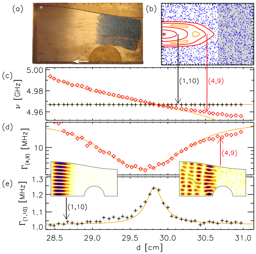
Figure 1: (color online). (a) Photograph of the cavity including a movable (white arrow) half disk, absorbers (gray), and antenna position (red). (b) Poincaré section along the upper boundary of the classical dynamics of the closed billiard with regular tori (red), a chaotic orbit (blue), and a $3$:$1$ nonlinear resonance chain (orange). The gray region indicates the absorbing part. (c) Frequency $\nu$ and (d), (e) width $\Gamma$ of the regular modes $(n,m)=(1,10)$ (black pluses) and $(4,9)$ (red diamonds) vs. half disk position $d$. Solid orange lines correspond to the $3\times 3$ matrix model, Eq. (3). Insets visualize numerically determined regular modes of the closed billiard.

direct regular-to-chaotic tunneling Dembowski et al. (2000); Hensinger et al. (2001); Steck et al. (2001); Fromhold et al. (2002); Bäcker et al. (2008b); Shinohara et al. (2010); Yang et al. (2010); Song et al. (2012); Shrestha et al. (2013). Recently, the coupling matrix element between two modes coupled by a nonlinear resonance chain was very nicely observed experimentally in the near integrable regime Kwak et al. (2015) in microcavities Yang et al. (2010). The experimental observation of the enhancement of regular-to-chaotic tunneling rates due to RAT, however, has remained open.

Here we measure the enhanced line width of regular modes due to RAT in an open microwave cavity; see Fig. 1(a). Couplings between different regular modes are caused by a large $3$:$1$ nonlinear resonance chain; see Fig. 1(b). We show the influence of RAT in two ways: (i) We induce RAT parametrically by a crossing of the frequencies of two regular modes under variation of the position of a half disk inset, see Figs. 1(c)-1(e); (ii) we explore the dependence of the width of regular modes towards the semiclassical limit, i.e., for increasing frequency. The characteristic plateau and peak structure of RAT is observed showing a good qualitative agreement with numerically determined tunneling rates using the closed system; see Fig. 2.

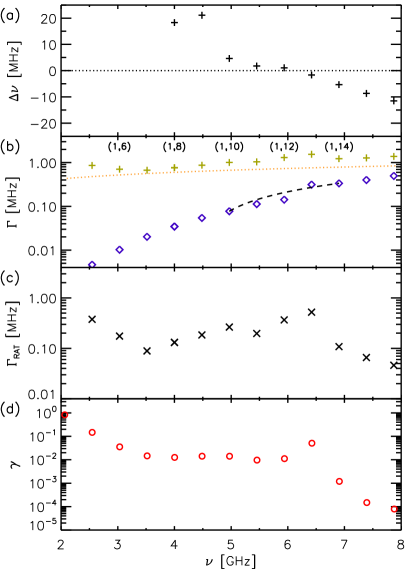
Figure 2: (color online). (a) Frequency difference $\Delta\nu=\nu_{(1,m)}-\nu_{(4,m-1)}$ of modes $(1,m)$ and $(4,m-1)$ for $m=8,\dots,16$ and fixed half disk position $d=30.0$ cm. The dotted line indicates the value 0. (b) Experimental widths $\Gamma_{(1,m)}$ (green pluses) of the inner mode for $m=5,\dots,16$, the square root dependence of $\Gamma_{\text{wall}}$ (orange dotted line), and $\Gamma_{\text{antenna}}$ (blue diamonds) with the dashed line showing the assumed linear dependence at the close encounter. (c) $\Gamma_{\text{RAT}}$ (black crosses) showing the initial exponential decay and the characteristic plateau and peak structure of RAT. (d) Numerical dimensionless tunneling rates $\gamma_{(1,m)}$ of the closed system (red open circles).

For the experimental realization we use a desymmetrized cosine Bäcker et al. (1997, 2002) microwave resonator Stöckmann and Stein (1990); Sridhar (1991); Gräf et al. (1992); So et al. (1995); Stöckmann (1999), with a large $3$:$1$ nonlinear resonance chain; see Fig. 1(a). The area enclosed by the resonance chain is approximately half of the area of the regular island, such that the characteristic plateau and peak structure of RAT is observable on top of the experimental line width. Figure 1(b) shows a Poincaré section with perpendicular momentum $|p_{\parallel}|/p\leq 1$ vs. arclength along the upper boundary of the cosine billiard consisting of regular tori, a chaotic orbit, and the $3$:$1$ nonlinear resonance chain. In the resonator (height $h=1$ cm, length $l=60$ cm, width left $w_{l}=30.96$ cm, and right $w_{r}=24$ cm) we placed a half disk (radius $r=9$ cm) at the bottom boundary with an adjustable distance $d$ from the left boundary, see Fig. 1(a). It destroys the hierarchical island structure and partial barriers in the chaotic region leading to a sharp separation of regular and chaotic dynamics. This reduces strong fluctuations of the tunneling rates, which would hinder the observation of RAT. Chaotic trajectories spread over the whole billiard also hitting the half disk, whereas the regular motion is confined to the region left of the half disk. The semiclassical eigenfunction hypothesis Percival (1973); Berry (1977); Voros (1979) predicts regular and chaotic eigenmodes of the billiard. Numerical examples of regular modes are shown in Figs. 1(d) and  1(e) (insets). In phase space they localize on quantizing tori at the starting point of the arrows in Fig. 1(b), as can be visualized by a Husimi representation Bäcker et al. (2002).

We open the system by introducing a broad band foam absorber on the right-hand side [grey shaded region in Fig. 1(b)] thus connecting the chaotic part to the continuum. The surviving chaotic modes concentrate on the remaining part of the chaotic region to the left of the absorber. This enables the observation of regular-to-chaotic tunneling by measuring the line width of a regular mode. A tedious extraction by analyzing many avoided crossings is not necessary Bäcker et al. (2008b).

The fixed antenna is placed at the upper left part of the billiard [red dot in Fig. 1(a)], guaranteeing a good excitation of all regular modes. The complex reflection amplitude $S_{11}(\nu)$ was measured as a function of the microwave frequency $\nu$. In the isolated resonance regime it can be described by the Breit-Wigner formula

$$S_{11}(\nu)=1-i\sum_{k}\frac{a_{k}}{\nu-\nu_{k}-\Delta_{k}+\frac{i}{2}\Gamma_{k}},$$ (1)

where the sum runs over all modes with eigenfrequency $\nu_{k}$ and eigenwidth $\Gamma_{k}$. Here $a_{k}=\text{Re}(\lambda_{k})\psi_{k}(\vec{r}_{1})\psi_{k}(\vec{r}_{1})$ is the residuum of the resonance, $\psi_{k}(\vec{r}_{1})$ the $k$th wave function at the antenna position $\vec{r}_{1}$, and $\lambda_{k}$ the coupling coefficient of the antenna. The real part of $\lambda_{k}$ describes the coupling to the continuum and the imaginary part induces a frequency shift $\Delta_{k}$. We will use the term mode for these resonances and reserve further on the term resonance to the nonlinear resonance chain.

The regular modes are labeled by two quantum numbers $(n,m)$, where $n$ counts the number of excitations in the horizontal and $m$ in the vertical direction. Their width $\Gamma_{(n,m)}$ contains different contributions

$$\Gamma_{(n,m)}=\Gamma_{\text{RAT}}+\Gamma_{\text{wall}}+\Gamma_{\text{antenna}},$$ (2)

where $\Gamma_{\text{RAT}}$ is the width enhancement due to regular-to-chaotic tunneling in the presence of the absorber. The width $\Gamma_{\text{wall}}$ is induced by the bottom and top plates and the side walls. The width induced by the antenna, $\Gamma_{\text{antenna}}=2|a_{(n,m)}|$, is given by the residuum $a_{(n,m)}$.

(i) RAT induced by parameter variation.—We first show the signature of RAT from parametric dependencies of two close-by regular modes. The modes $(n,m)=(1,10)$ and $(n^{\prime},m^{\prime})=(4,9)$ (Fig. 1 insets) are coupled via to the nonlinear $3$:$1$ resonance chain, as $n^{\prime}=n+3$ and $m^{\prime}=m-1$. We measure $S_{11}(\nu)$ for several half disk positions $d$, fixing all other parameters. We fitted their frequency $\nu$ and width $\Gamma$, giving the parametric dependencies shown in Figs. 1(c)-1(e). We observe a crossing of the frequencies and an avoided crossing of the widths. An increase of the width of the mode $(1,10)$, lying deep inside the regular region, is observed once the mode $(4,9)$ is close by, which is a clear signature of RAT.

A quantitative description of all features displayed in Fig. 1 can be obtained in terms of a matrix model. We start with a $2\times 2$ matrix description of the two regular modes with diagonal elements $E_{1}-i\gamma_{1}/2$ and $E_{4}(d)-i\gamma_{4}/2$, where $E_{1}$ and $E_{4}$ are the eigenenergies of the uncoupled modes, $(1,10)$ and $(4,9)$. As the inner mode concentrates away far off the half disk, we assume $E_{1}$ to be independent of $d$. Close to the crossing we assume a linear dependence on the frequency axis of $E_{4}(d)$ as is suggested by Fig. 1(c). The widths $\gamma_{1}$ and $\gamma_{4}$ are assumed to be independent of $d$ as they are due to antenna coupling and wall absorption. An off-diagonal matrix element $V_{3:1}$ describes the coupling via the 3:1 nonlinear resonance chain. The line width of mode 1, obtained by diagonalizing the $2\times 2$ matrix, increases at the point of degeneracy of the real parts of the two modes, as exhibited in Fig. 1(e). This is a manifestation of the coupling of two regular modes via a nonlinear resonance chain.

For a full analysis of RAT, however, one additionally has to consider the tunneling into the chaotic region. If the two-mode model were the full truth, the curves in Figs. 1(d) and 1(e) should be just mirror images of each other because of the invariance of the trace of the Hamilton matrix. Thus the sum of the two line widths should be independent of $d$, which obviously is not the case. Thus there must be (at least) one other mode from the chaotic region involved. We assume a linear dependence of $E_{\text{ch}}(d)$ due to the change of the area to the left of the absorber causing an average drift in mode energies, described by a Taylor expansion up to linear order in $d$. The width $\gamma_{\text{ch}}$ is assumed to be constant.

Because of coupling with mode 4 its width dependence with $d$ must be essentially the mirror image of Fig. 1(d), since the contribution of mode 1 to the width is only marginal. Hence the chaotic mode has to become broad at the crossing point, while at the same time the width of mode 4 becomes small. This is the phenomenology which is known in other contexts as resonance trapping Rotter (2009); Persson et al. (2000). It is found whenever an effective Hamiltonian of the form $H=H_{0}-iWW^{\dagger}$ is involved. Here $H_{0}$ is the Hamiltonian of the unperturbed system, and $W$ is a $N\times M$ coupling matrix, where $N$ is the number of modes taken into account and $M$ is the number of open channels (here $N=3$ and $M\approx 6$ is obtained by dividing the length of the absorbing edge by $\lambda/2$). This suggests an ansatz of the Hamiltonian in terms of a $3\times 3$ matrix,

$$H=\left(\begin{matrix}E_{1}-i\dfrac{\gamma_{1}}{2}&V_{3:1}&0\\ V_{3:1}&E_{4}(d)-i\dfrac{\gamma_{4}}{2}&-iV_{\text{dir},4}\\ 0&-iV_{\text{dir},4}&E_{\text{ch}}(d)-i\dfrac{\gamma_{\text{ch}}}{2}\end{matrix}\right).$$ (3)

This ansatz assumes ($\alpha$) that the direct tunneling coupling of mode 1 to the chaotic region is negligible for the frequency range of Fig. 1 and ($\beta$) that the direct tunneling coupling of mode 4 to the chaotic region dominantly appears in the coupling of mode 4 to the open channels encoded in the second row of $W$ (and much less in the coupling of mode 4 to the chaotic mode in $H_{0}$). As the real parts of modes 1 and 4 cross, with no indication of an avoided crossing [Fig. 1(c)], the off-diagonal elements of $H$ have to be either real or imaginary, but not complex. After diagonalization of the $3\times 3$ Hamiltonian we have to compare the complex quantum mechanical eigenenergies $\tilde{E}=E-i{\gamma}/{2}$ with the experimentally measured complex electromagnetic eigenvalues $\tilde{\nu}=\nu-i\Gamma/2$ by their complex wave number $\tilde{E}/(\hbar^{2}/2M)=(2\pi\tilde{\nu}/c)^{2}$, yielding

$$E=\nu^{2}\cdot(2\pi/c)^{2};\quad\gamma=2\nu\Gamma\cdot(2\pi/c)^{2},$$ (4)

where we use units $\hbar/2M=1$ and $\Gamma\ll\nu$. Fitting the experimental data gives the solid orange lines in Figs. 1(c)-1(e) and yields the parameters of the model . In particular, this gives for the matrix element $V_{3:1}=2.3\,\text{m}^{-2}$, which is of the same order as the prediction for the closed system, $V_{3:1,\text{cl}}=0.51\,\text{m}^{-2}$ .

We would like to emphasize that the third chaotic mode is an effective description of the coupling of the system to the environment, more precisely speaking to the absorber. For the example of Fig. 1 we chose a situation where the effective broad chaotic mode crosses almost at the same $d$ value where the two regular modes cross. For other quantum numbers $m$ the situation was comparable but the crossing of the chaotic state was further apart. We find a similar value for $V_{3:1}$ using a reduced $2\times 2$ model, as this value is defined mainly by the width increase of $\Gamma_{(1,10)}$ close to $d=29.8$ cm. We considered either a constant width $\Gamma_{4}$ using only the range 29.5 cm $\leq d\leq 30.0$ cm, or an adjusted cosine or Gaussian width dependence $\Gamma_{4}(d)$ for the whole range of $d$. This shows that the signature of RAT in Fig. 1(e) can be quantitatively understood.

(ii) RAT plateau and peak structure.—A key feature of RAT is the plateau and peak structure on top of the exponential decay of the tunneling rates towards the semiclassical limit. We observe this signature of RAT with fixed half disk position $d=30.0$ cm. The plateau should appear when in addition to the inner mode $(1,m)$ the outer mode $(4,m-1)$ starts to exist ($m\geq 8$). A peak is expected at the crossing of these modes for increasing $m$, as seen in Fig. 2(a) for the frequency difference $\Delta\nu=\nu_{(1,m)}-\nu_{(4,m-1)}$ around 6 GHz. There the corresponding quantizing tori in phase space are symmetric with respect to the nonlinear resonance chain. From the measured widths $\Gamma_{(1,m)}$ [green pluses in Fig. 2(b)] for $m=5,\dots,16$ we subtract, according to Eq. (2), the width contributions $\Gamma_{\text{wall}}$ and $\Gamma_{\text{antenna}}$ (discussed below) and the resulting contribution $\Gamma_{\text{RAT}}$ is shown as black crosses in Fig. 2(c). For low frequencies up to 3.5 GHz an exponential dependence is obtained, as expected from direct regular-to-chaotic tunneling. RAT becomes visible from 4 GHz on as a broad plateau ($m\geq 8$) ending in a peak structure around 6.5 GHz.

For numerical comparison, tunneling rates were determined using the closed system in a similar way as described in Ref. Bäcker et al. (2008b). Extending the chaotic region by varying the height of a rectangle that was attached to the bottom of the cosine billiard at $x>30\,\text{cm}$, tunneling rates $\gamma_{(1,m)}$ are determined by evaluating avoided crossings between the regular mode $(1,m)$ and chaotic modes [Fig. 2(d)]. Qualitatively these rates are in good agreement with the experimental results $\Gamma_{\text{RAT}}$ in Fig. 2(c). A quantitative comparison is difficult, as $\Gamma_{\text{RAT}}$ depends also on the wall and antenna contributions $\gamma_{4}$ and $\gamma_{\text{ch}}$ which differ for each $m$. However, the experimental and numerical frequency ranges for the initial exponential decay, the plateau, and the peak are identical.

Let us finally discuss the wall and antenna contributions $\Gamma_{\text{wall}}$ and $\Gamma_{\text{antenna}}$ in Fig. 2(b). The wall absorption $\Gamma_{\text{wall}}$ has a square root frequency dependence due to nonperfect conductance of the cavity walls Jackson (1962). It was extracted from measurements of the closed cavity, where the absorber was removed and the right part of the billiard was closed. We find $\Gamma_{\text{wall}}=0.30$ MHz$\sqrt{\nu/\text{GHz}}$; see the orange dotted line in Fig. 2(b). The width $\Gamma_{\text{antenna}}=2|a_{(1,m)}|$ induced by the antenna is shown as blue diamonds in Fig. 2(b) and is extracted by fitting a Lorentzian to the measured resonance. Around 6 GHz, where the frequency difference $\Delta\nu$ in Fig. 2(a) is small, modes 1 and 4 are coupled, such that the extracted $\Gamma_{\text{antenna}}$ is affected. In this regime we therefore interpolate it by a linear increase; see the dashed line in Fig. 2(b). The overall monotonic increase of $\Gamma_{\text{antenna}}$ is due to two effects: ($\alpha$) the antenna length is small compared to the wavelength leading to small and increasing antenna coupling $\text{Re}(\lambda)$, and ($\beta$) the distance of the antenna to the wall is smaller than a quarter of the wavelength such that the wave function increases monotonically at the antenna position.

In this Letter, we experimentally observe RAT in a generic mixed phase space using an opened microwave billiard. We demonstrate RAT by the width increase of the exemplary mode $(1,10)$ when it is crossed by mode $(4,9)$. With a $3\times 3$ matrix model the coupling matrix element $V_{3:1}$ is extracted, which is of the same order as the theoretical value. Second, measuring the widths of the modes $(1,m)$ for increasing $m$ reveals the regimes of direct regular-to-chaotic tunneling with an exponential decay and RAT with its characteristic plateau and peak structure. This experimental work motivates future theoretical studies for a better quantitative description of RAT, in particular using semiclassical methods Shudo and Ikeda (1995); Mertig et al. (2013).