On the definition of entanglement entropy in lattice gauge theories

Abstract

We focus on the issue of proper definition of entanglement entropy in lattice gauge theories, and examine a naive definition where gauge invariant states are viewed as elements of an extended Hilbert space which contains gauge non-invariant states as well. Working in the extended Hilbert space, we can define entanglement entropy associated with an arbitrary subset of links, not only for abelian but also for non-abelian theories. We then derive the associated replica formula. We also discuss the issue of gauge invariance of the entanglement entropy. In the $Z_{N}$ gauge theories in arbitrary space dimensions, we show that all the standard properties of the entanglement entropy, e.g. the strong subadditivity, hold in our definition. We study the entanglement entropy for special states, including the topological states for the $Z_{N}$ gauge theories in arbitrary dimensions. We discuss relations of our definition to other proposals.

1 Introduction

Entanglement entropy plays important roles in various fields of quantum physics including string theoryt4 ; t1 ; sw1 ; sw2 ; r ; t2 ; t3 ; t5 , condensed matter physicswen ; pre ; mul ; hal ; wen2 ; gon2 , and the physics of the black hole sus ; kab1 ; kab2 ; sh1 ; sh2 . It is believed that entanglement entropy characterizes various aspects of quantum states in a simple and unified manner.

In the context of lattice gauge theories, entanglement entropy is expected to be a useful tool for studying confinement / deconfinement transitions (or crossover) NT ; dcp ; lv . It has been pointed out, however, that there is a subtle problem in the definition of entanglement entropy in gauge theoriesCHR2013 ; Radicevic2014 ; Donnelly2012 ; Don . When we calculate the entanglement entropy of a region $V$, we first express the Hilbert space of the total system as a tensor product of the Hilbert spaces of $V$ and that of $\bar{V}$, the complement of $V$. Thus we trace out the degrees of freedom of $\bar{V}$ and obtain the reduced density matrix of $V$. For gauge theories, however, the physical gauge invariant Hilbert space can not be factorized into a tensor product of the gauge invariant subspaces of $V$ and that of $\bar{V}$ due to the local gauge invariance at the boundary $\partial V$ between $V$ and $\bar{V}$. This reflects the fact that the fundamental physical degrees of freedom contain Wilson loops, which are nonlocal operators. Due to the absence of the factorization into a tensor product, it is not straightforward to define the reduced density matrix of some region and to calculate the entanglement entropy. We need to specify the prescription to obtain the reduced density matrix of the region.

In this paper, we propose a definition of the entanglement entropy in lattice gauge theories. We extend the gauge invariant Hilbert space to a larger Hilbert space in order to admit the factorization into a tensor product of the gauge invariant subspaces of the region $V$ and the region $\bar{V}$ in this larger Hilbert space. The natural candidate of this larger Hilbert space is the whole (gauge non-invariant) Hilbert space of the link variables. We then obtain the reduced density matrix of the region $V$ by tracing out the link variables of the region $\bar{V}$. We define the entanglement entropy as the von Neumann entropy of the above reduced density matrix. We can define the entanglement entropy for an arbitrary subset of links. This definition is applicable not only for abelian theories but also for non-abelian ones. We then derive the replica formula to calculate the entanglement entropy in our definition.

In the $Z_{N}$ gauge theories in arbitrary space dimensions, we express the whole Hilbert space by useful basis states, which are eigenstates of the gauge transformations Radicevic2014 . We argue that all the standard properties of entanglement entropy, e.g. the strong subadditivity, hold in our definition. We study the one for some special states. In particular, we calculate rigorously the one for the topological states in arbitrary space dimensions. We discuss relations of our definition to other proposals. We also demonstrate that the entanglement entropy depends on the choice of the gauge fixing for some simple cases. This indicates that one should not fix the gauge, at least on the boundary points between two regions, to calculate the entanglement entropy in gauge theories.

The present paper is organized as follows. In section 2, we give precise definitions of the geometry of our lattice and define the entanglement entropy. We discuss the gauge invariance of the reduced density matrix. We also derive the replica formula here. In section 3, we consider the $Z_{N}$ gauge theories. We express the whole Hilbert space by eigenstates of the gauge transformations, and derive an explicit expression of the entanglement entropy. We then argue that all the standard properties of entanglement entropy, e.g. the strong subadditivity, hold in our definition. We study the one for some special states. In particular, we calculate the one for the topological states in arbitrary space dimensions. We discuss relations of our definition to other proposals. In section 4, we summarize our investigations. Some properties of the $Z_{N}$ gauge theories used in the main text are given in appendix A, while gauge invariant states in non-abelian gauge theories are briefly discussed in B.

2 Naive definition of entanglement entropy in lattice gauge theories

2.1 Definition and some properties

Geometry

We can treat quite general geometries and boundary conditions.

Our lattice is $(\mathcal{S},\mathcal{L})$, where $\mathcal{S}$ denotes the set of sites $x,y,\ldots\in\mathcal{S}$, and $\mathcal{L}\subset\mathcal{S}\times\mathcal{S}$ the set of links. We understand that $\ell=(x,y)$ and $\bar{\ell}=(y,x)$ are different ways of expressing a single link in $\mathcal{L}$. This in particular means that $\ell\in V$ implies $\bar{\ell}\in V$ for any subset $V\subset\mathcal{L}$. Here we do not assume a particular structure of our lattice such as regularity, so that a random lattice could be treated. Note that this setup can treat both periodic and free boundary conditions for the whole lattice.

We define the boundary of a subset $V\subset\mathcal{L}$ as

$$\partial V:=\bigl{\{}\,x\in\mathcal{S}\,\bigl{|}\,\text{$(x,y)\in V$ and $(x,z)\in\bar{V}$ for some $y,z\in\mathcal{S}$}\,\bigr{\}},$$ (1)

which is the set of sites in both $V$ and its complement $\bar{V}=\mathcal{L}\backslash V$. Note also that $\partial V=\partial\bar{V}$.

Naive definition of entanglement entropy

We consider the global density matrix $\rho$ for gauge theories, whose elements are denoted by

$$\langle U|\rho|U^{\prime}\rangle \equiv \rho(U;U^{\prime})=\rho(U_{V},U_{\bar{V}};U_{V}^{\prime},U_{\bar{V}}^{\prime})$$ (2)

where $U$ represents a gauge configuration (a set of all link variables), $U=\{U_{\ell}\ |\ \ell\in\mathcal{L}\}$, while $U_{V},U_{\bar{V}}$ are gauge configurations on $V$ and $\bar{V}$, $U_{V}=\{U_{\ell}\ |\ \ell\in V\}$ and $U_{V}=\{U_{\ell}\ |\ \ell\in\bar{V}\}$, respectively.

We propose to define a reduced density matrix as

$$\langle U_{V}|\rho_{V}|U_{V}^{\prime}\rangle\equiv\rho_{V}(U_{V};U^{\prime}_{V}) = \int{\cal D}U_{\bar{V}}\,\rho(U_{V},U_{\bar{V}};U_{V}^{\prime},U_{\bar{V}}),$$ (3)

where ${\cal D}U_{\bar{V}}$ denotes a product of the group invariant integrals or sums. For the compact group, we have ${\cal D}U_{\bar{V}}=\prod_{\ell\in\bar{V}}dU_{\ell}$, where $dU_{\ell}$ is the Haar measure for the link variable $U_{\ell}$.

The above definition of the reduced density matrix is a simple generalization of the reduced density matrix in spin systems, where the whole Hilbert space is a direct product of those of region $V$ and region $\bar{V}$, ${\cal H}={\cal H}_{V}\otimes{\cal H}_{\bar{V}}$. In the case of gauge theories, on the other hand, due to the local gauge invariance, the gauge invariant full Hilbert space can not be factorized into a product of gauge invariant subspaces, ${\cal H}_{\mathcal{L}}^{\rm inv}\not={\cal H}_{V}^{\rm inv}\otimes{\cal H}_{\bar{V}}^{\rm inv}$. Therefore the above reduced density matrix $\rho_{V}$ can not be obtained from a single partial trace of $\rho$ over the gauge invariant subspace ${\cal H}_{\bar{V}}^{\rm inv}$. Without gauge invariance, however, the whole Hilbert space can be factorized as ${\cal H}_{\mathcal{L}}={\cal H}_{V}\otimes{\cal H}_{\bar{V}}$, so that our definition of $\rho_{V}$ above can be understood as the partial trace of $\rho$ over the gauge non-invariant subspace ${\cal H}_{\bar{V}}$ on $U_{\bar{V}}$. In the next section, we explicitly construct the reduced density matrix for the $Z_{N}$ gauge theories in an arbitrary dimensions, and explicitly construct an extension of $\rho_{V}$ to ${\cal H}_{\mathcal{L}}={\cal H}_{V}\otimes{\cal H}_{\bar{V}}$.

From the reduced density matrix, the entanglement entropy can thus be defined as

$$S(V) = -\text{tr}\,[\rho_{V}\log\rho_{V}],$$ (4)

where the trace is taken over ${\cal H}_{V}$. The definitions (3) and (4) are so simple that they can be used not only for discrete abelian theories but also for continuous non-abelian gauge theories without practical difficulties.

In the next section, we will see that this trace is reduced to a sum of traces in the gauge invariant subspace ${\cal H}_{V}^{\rm inv}\subset{\cal H}_{V}$ and discuss that a basic properties such as the symmetric property and the strong subadditivity are satisfied for the $Z_{N}$ gauge theories.

Gauge invariance

In gauge theories, the global density matrix is gauge invariant as

$$\rho(U^{g};{U^{\prime}}^{h})=\rho(U;U^{\prime}),$$ (5)

where the gauge transformation of the link variable $U_{\ell}$ is given by $U_{\ell}^{g}=g_{x}U_{\ell}g_{y}^{\dagger}$ with $\ell=(x,y)$.

On the other hand, the reduced density matrix $\rho_{V}$ in  (3) does not have such a gauge invariance. Indeed,

$$\rho_{V}(U_{V}^{g_{V}};{U^{\prime}_{V}}^{h_{V}}) = \int{\cal D}U_{\bar{V}}\,\rho(U_{V}^{g_{V}},U_{\bar{V}};{U_{V}^{\prime}}^{h_{V}},U_{\bar{V}})=\int{\cal D}U_{\bar{V}}^{g_{\bar{V}}}\,\rho(U_{V}^{g_{V}},U_{\bar{V}}^{g_{\bar{V}}};{U_{V}^{\prime}}^{h_{V}},U_{\bar{V}}^{g_{\bar{V}}})$$ (6)

$$= \int{\cal D}U_{\bar{V}}\,\rho(U_{V},U_{\bar{V}};(U_{V}^{\prime})^{h_{V}g_{V}^{-1}},U_{\bar{V}})=\rho_{V}(U_{V};(U^{\prime}_{V})^{h_{V}g_{V}^{-1}}),$$

where the invariance of the measure ${\cal D}U_{\bar{V}}^{g_{\bar{V}}}={\cal D}U_{\bar{V}}$ and the gauge invariance of the full density matrix $\rho$ such as

$$\rho(U_{V}^{g_{V}},U_{\bar{V}}^{g_{\bar{V}}};{U_{V}^{\prime}}^{g_{V}},U_{\bar{V}}^{g_{\bar{V}}}) = \rho(U_{V},U_{\bar{V}};U_{V}^{\prime},U_{\bar{V}})$$ (7)

are used. Therefore $\rho_{V}$ is invariant under diagonal gauge transformations ($g_{V}=h_{V}$) only.

This suggests that the reduced density matrix and thus its entanglement entropy may depend on the choice of the gauge if the gauge fixing is employed in the calculation. Indeed, we will show in the next section that values of the entanglement entropy are different for different gauge fixing conditions in some simple cases for the $Z_{N}$ gauge theories. Because of this problem, it is important and sensible to calculate the entanglement entropy in the gauge invariant way without gauge fixing.

2.2 Replica formula

We briefly consider the replica formula for the entanglement entropy of lattice gauge theories based on our definition.

Transfer matrix and path integral

In lattice gauge theories, the evolution in a discrete time is given by the transfer matrix $\hat{T}$ (for example, see Refs. Creutz1977 ; Luescher1977 ), which is given by

$$T(U,U^{\prime}):=\langle U|\hat{T}|U^{\prime}\rangle=\exp[\frac{1}{2}S_{d}(U)]\exp[S_{0}(U,U^{\prime})]\exp[\frac{1}{2}S_{d}(U^{\prime})]$$ (8)

where

$$S_{d}(U) = \frac{1}{2g^{2}}\sum_{x\in\mathcal{S}}\mathop{\sum_{\mu=1,\nu=1}}_{\mu\not=\nu}^{d}\text{Tr}\,\left[U_{x,\mu}U_{x+\hat{\mu},\nu}U_{x+\hat{\nu},\mu}^{\dagger}U_{x,\nu}^{\dagger}\right]:=\frac{1}{2g^{2}}\sum_{x\in\mathcal{S}}\mathop{\sum_{\mu=1,\nu=1}}_{\mu\not=\nu}^{d}P_{\mu\nu}(x),$$ (9)

$$S_{0}(U,U^{\prime}) = \frac{1}{2g^{2}}\sum_{x\in\mathcal{S}}\sum_{\mu=1}^{d}\text{Tr}\left[U_{x,\mu}(U^{\prime}_{x,\mu})^{\dagger}+U_{x,\mu}^{\prime}(U_{x,\mu})^{\dagger}\right]$$ (10)

for the plaquette action on a $d$-dimensional hyper-cubic lattice with the coupling constant $g$. We here define $P_{\mu\nu}(x)$ as a trace of the plaqiutte on $\mu\nu$ plane at $x$, and use the notation that $U_{x,\mu}:=U_{\ell}$ with $\ell=(x,x+\hat{\mu})$ and $\hat{\mu}$ is an unit vector in the $\mu$ direction.

The wave function for the vacuum state is obtained as

$$\lim_{N_{T}\rightarrow\infty}\langle U|\hat{P}(\hat{T})^{N_{T}}|\Psi\rangle = \langle U|0\rangle\langle 0|\Psi\rangle$$ (11)

for an arbitrary gauge invariant state $|\Psi\rangle$ which satisfies $\langle 0|\Psi\rangle\not=0$, where $\hat{P}$ is a projection to the physical (gauge invariant) Hilbert space as

$$\hat{P}:=\prod_{x\in\mathcal{S}}\int dg_{x}\,\hat{E}_{x}(g_{x}).$$ (12)

Here $\hat{E}_{x}(g_{x})$ generates the gauge transformation at $x$ by $g_{x}$. Note that $(\hat{P})^{2}=\hat{P}$ and $[\hat{T},\hat{P}]=0$. While we explicitly write $\hat{P}$ in the above expression since $\langle U|$ is not gauge invariant, the formula without $\hat{P}$ is equaly correct since $\hat{P}|\Psi\rangle=|\Psi\rangle$.

Thus we can write

$$\langle U|\hat{P}(\hat{T})^{N_{T}}|U^{\prime}\rangle = \exp\left[\frac{1}{2}S_{d}(U)\right]\int_{U[0]=U^{\prime}}^{U[N_{T}]=U}{\cal D}U[t]\exp\left[S_{G}(U[t])\right]\exp\left[\frac{1}{2}S_{d}(U^{\prime})\right]$$ (13)

where

$${\cal D}U[t] := \prod_{t=1}^{N_{T}-1}\prod_{\ell\in\mathcal{L}}dU_{\ell}[t]\prod_{t=0}^{N_{T}}\prod_{x\in\mathcal{S}}dg_{x}[t]$$ (14)

$$S_{G}(U[t]) := \sum_{t=1}^{N_{T}-1}S_{d}(U[t])+\sum_{t=1}^{N_{T}}S_{0}(U^{g}[t-1],U^{g}[t])$$ (15)

where $U_{x,\mu}^{g}[t]=g_{x}[t]U_{x,\mu}[t]g_{x+\hat{\mu}}^{\dagger}[t]$. Defining a new gauge field as $U_{z,0}:=g_{x}^{\dagger}[t]g_{x}[t+1]$ where $z=(x,t)$ is a $d+1$ dimensional lattice point, and introducing a new notation for gauge fields $U_{z,\mu}$ with $\mu=0,1,\cdots d$, we have

$$\langle U_{d}|\hat{P}(\hat{T})^{N_{T}}|U_{d}^{\prime}\rangle = \exp\left[\frac{1}{2}S_{d}(U_{d})\right]\int_{U_{z_{0}}=U_{d}^{\prime}}^{U_{z_{T}}=U_{d}}{\cal D}U\int{\cal D}g_{z_{0}}\exp\left[S_{\rm plaq}(U_{d})\right]\exp\left[\frac{1}{2}S_{d}(U^{\prime})\right]$$

where

$$S_{\rm plaq}(U) = \frac{1}{2g^{2}}\sum_{x\in\mathcal{S}}\Bigl{[}\sum_{t=1}^{N_{T}-1}\mathop{\sum_{\mu=0,\nu=0}}_{\mu\not=\nu}^{d}P_{\mu\nu}(z)+\sum_{k=1}^{d}\left\{P_{0k}(z_{0})+P_{k0}(z_{0})\right\}\Bigr{]},$$ (17)

with $z_{0}=(x,0)$ and $z_{T}=(x,N_{T})$. Here $U_{z_{0}}=U_{d}$ means $U_{z_{0},k}=(U_{d})_{x,k}$ for $k=1,2,\cdots,d$. Note that since $S_{\rm plaq}$ and $S_{d}$ do not depend on $g_{z_{0}}$, the gauge transformation left after the change of variables, we have $\int{\cal D}g_{z_{0}}=1$ in the above expression.

Path integral expression

The (unnormalized) density matrix for the vacuum state, can be obtain as

$$\langle U_{d}|\hat{\rho}|U_{d}^{\prime}\rangle = e^{\frac{1}{2}[S_{d}(U_{d})+S_{d}(U_{d}^{\prime})]}\lim_{N_{T}\rightarrow\infty}\int{\cal D}U\delta(U_{z_{0}^{-}}-U_{d})\delta(U_{z_{0}^{+}}-U_{d}^{\prime})e^{S_{\rm plaq}(U)}$$ (18)

$$\times e^{\frac{1}{2}[S_{d}(U_{z_{T}^{+}})+S_{d}(U_{z_{T}^{-}})]}$$

where $x\in\mathcal{S}$, $-N_{T}\leq t\leq N_{T}$, $z_{0}^{\pm}=(x,0^{\pm})$, and $z_{T}^{\pm}=(x,\pm N_{T})$.

In practice, one often employs the periodic boundary condition at $\pm N_{T}$ in the Euclidian time, which correspond to the thermal density matrix at temperature $T=1/(2N_{T}a)$, where $a$ is the lattice spacing. In this case, after interchanging $t=0$ and $t=\pm N_{T}$, we have

$$\langle U_{d}|\hat{\rho}^{T}|U_{d}^{\prime}\rangle = e^{\frac{1}{2}[S_{d}(U_{d})+S_{d}(U_{d}^{\prime})]}\int_{U_{z_{T}^{-}}=U_{d}^{\prime}}^{U_{z_{T}^{+}}=U_{d}}{\cal D}Ue^{S_{\rm plaq}^{T}(U)}$$ (19)

where

$$S^{T}_{\rm plaq}(U)=\frac{1}{2g^{2}}\sum_{x\in\mathcal{S}}\Bigl{[}\sum_{t=-N_{T}+1}^{N_{T}-1}\mathop{\sum_{\mu=0,\nu=0}}_{\mu\not=\nu}^{d}P_{\mu\nu}(z)+\sum_{k=1}^{d}\left\{P_{0k}(z_{T}^{-})+P_{k0}(z_{T}^{-})\right\}\Bigr{]}.$$ (20)

The density matrix for the vacuum state is reproduced from $\hat{\rho}^{T}$ by the $T\rightarrow 0$ limit.

Reduced density matrix for replica formula

We now consider two regions $V$ and $\bar{V}=\mathcal{L}\backslash V$, and denote $U=(U_{V},U_{\bar{V}})$ and $U_{d}=(U_{d}{}_{V},U_{d}{}_{\bar{V}})$. Then the reduced density matrix $\hat{\rho}_{V}^{T}$ can be written as

$$\rho_{V}^{T}(U_{d}{}_{V};U_{d}^{\prime}{}_{V}):=\langle U_{d}{}_{V}|\hat{P}\hat{\rho}_{V}^{T}|U_{d}^{\prime}{}_{V}\rangle = \int_{U_{z_{T}^{-}}{}_{V}=U_{d}^{\prime}{}_{V}}^{U_{z_{T}^{+}}{}_{V}=U_{d}{}_{V}}{\cal D}Ue^{\frac{1}{2}[S_{d}(U_{d})+S_{d}(U_{d}^{\prime})]}e^{S_{\rm plaq}^{T}(U)}.$$ (21)

The replica formula for the entanglement entropy in now given as

$$S(V) = \lim_{n\rightarrow 1}\frac{1}{1-n}\log\left(\frac{Z_{n}}{Z_{1}^{n}}\right),\qquad Z_{n}:=\text{Tr}(\hat{\rho}_{V}^{T})^{n}$$ (22)

where $Z_{n}$ can be expressed in the path-integral as

$$Z_{n} = \left(\prod_{i=1}^{n}\int{\cal D}U_{i}\right)\rho_{V}^{T}(U_{1};U_{2})\rho_{V}^{T}(U_{2};U_{3})\cdots\rho_{V}^{T}(U_{n};U_{1})$$ (23)

and $\rho_{V}^{T}(U_{i},U_{j})$ is given in (21). Note that (23) is invariant under the local gauge transformation $g$ in $d+1$ dimensions with the period $2N_{T}$ ( not $2nN_{T}$) at the boundary, which satisfies

$$\qquad g_{(x,2kN_{T})}=g_{(x,0)}\quad\rm{at}\ x\in\partial V,\qquad k=1,2,\cdots,n.$$ (24)

3 $Z_{N}$ gauge theories in an arbitrary dimension

We consider the $Z_{N}$ gauge theories in this section.

3.1 Some properties of divergence-free flux-configurations

Flux-configuration

For each link $\ell\in\mathcal{L}$, we associate a flux $k_{\ell}\in\{0,1,\ldots,N-1\}$. We assume the consistency $k_{\ell}=-k_{\bar{\ell}}$. Here and throughout the present paper, equalities for the flux are with respect to mod $N$. We denote by $\boldsymbol{k}=(k_{\ell})_{{\ell\in\mathcal{L}}}$ a configuration of flux over the whole lattice which satisfies $d_{x}^{\mathcal{L}}(\boldsymbol{k})=0$ at ${}^{\forall}x\in\mathcal{S}$, where

$$d_{x}^{\mathcal{L}}(\boldsymbol{k}):=\mathop{\sum_{y\in\mathcal{S}}}_{{\rm s.t.}\,(x,y)\in\mathcal{L}}k_{(x,y)}.$$ (25)

is the divergence of $\boldsymbol{k}$ at $x$ associated with region $\mathcal{L}$. We denote the set of all divergent-free $\boldsymbol{k}$’s by $\tilde{\mathcal{F}}$.

Take an arbitrary subset $V\subset\mathcal{L}$. For any $\boldsymbol{k}\in\tilde{\mathcal{F}}$, let $R_{V}(\boldsymbol{k})$ be the configuration obtained by omitting all the flux outside $V$. We then denote by $\tilde{\mathcal{F}}_{V}$ the set of $\boldsymbol{k}^{\prime}$ which is written as $\boldsymbol{k}^{\prime}=R_{V}(\boldsymbol{k})$ for some (not necessarily unique) $\boldsymbol{k}\in\tilde{\mathcal{F}}$.

Incoming flux and decomposition of $\tilde{\mathcal{F}}$

Fix an arbitrary subset $V\subset\mathcal{L}$. For any $\boldsymbol{k}\in\tilde{\mathcal{F}}$, we define

$$\boldsymbol{f}_{V}(\boldsymbol{k}):=\bigl{(}d_{x}^{V}(\boldsymbol{k})\bigr{)}_{x\in\partial V},$$ (26)

where $d_{x}^{V}$ is the divergence associated with the region $V$, obtained by replacing $\mathcal{L}\to V$ in (25). Note that $\boldsymbol{f}_{V}(\boldsymbol{k})$ is the list of incoming flux at each site on the boundary $\partial V$. Recalling that $\partial V=\partial\bar{V}$ for $\bar{V}=\mathcal{L}\backslash V$, we have

$$\boldsymbol{f}_{V}(\boldsymbol{k})=-\boldsymbol{f}_{\bar{V}}(\boldsymbol{k}),$$ (27)

which represents the conservation of flux at the boundary sites.

For a give subset $V\subset\mathcal{L}$, we say that $\boldsymbol{f}\in\{0,1,\ldots,N-1\}^{\partial V}$ is admissible if there exists at least one $\boldsymbol{k}\in\tilde{\mathcal{F}}$ such that $\boldsymbol{f}_{V}(\boldsymbol{k})=\boldsymbol{f}$. Then we have a natural decomposition

$$\tilde{\mathcal{F}}=\bigcup_{\boldsymbol{f}}\tilde{\mathcal{F}}^{(\boldsymbol{f})},$$ (28)

where the union is over all admissible $\boldsymbol{f}$, and

$$\tilde{\mathcal{F}}^{(\boldsymbol{f})}:=\bigl{\{}\,\boldsymbol{k}\in\tilde{\mathcal{F}}\,\bigl{|}\,\text{$\boldsymbol{f}_{V}(\boldsymbol{k})=\boldsymbol{f}$}\,\bigr{\}}.$$ (29)

It is remarkable that all $\tilde{\mathcal{F}}^{(\boldsymbol{f})}$ with admissible $\boldsymbol{f}$ are completely isomorphic to each other. To see this, take arbitrary $\boldsymbol{f}_{1}$ and $\boldsymbol{f}_{2}$ which are admissible. Choose and fix $\boldsymbol{k}_{1},\boldsymbol{k}_{2}\in\tilde{\mathcal{F}}$ such that $\boldsymbol{f}_{V}(\boldsymbol{k}_{i})=\boldsymbol{f}_{i}$ for $i=1,2$. Then we define a map $\varphi_{1,2}:\tilde{\mathcal{F}}^{(\boldsymbol{f}_{1})}\to\tilde{\mathcal{F}}^{(\boldsymbol{f}_{2})}$ by $\varphi_{1,2}(\boldsymbol{k}):=\boldsymbol{k}-\boldsymbol{k}_{1}+\boldsymbol{k}_{2}$ and its inverse map $\varphi_{2,1}:\tilde{\mathcal{F}}^{(\boldsymbol{f}_{2})}\to\tilde{\mathcal{F}}^{(\boldsymbol{f}_{1})}$ by $\varphi_{2,1}(\boldsymbol{k}):=\boldsymbol{k}-\boldsymbol{k}_{2}+\boldsymbol{k}_{1}$. Since $\varphi_{1,2}(\boldsymbol{k}_{a})\not=\varphi_{1,2}(\boldsymbol{k}_{b})$ for $\boldsymbol{k}_{a}\not=\boldsymbol{k}_{b}$, $\boldsymbol{k}_{a,b}\in\tilde{\mathcal{F}}^{(\boldsymbol{f}_{1})}$ and a similar property for $\varphi_{2,1}$, these maps establish a one-to-one correspondence between the elements of $\tilde{\mathcal{F}}^{(\boldsymbol{f}_{1})}$ and $\tilde{\mathcal{F}}^{(\boldsymbol{f}_{2})}$: $\tilde{\mathcal{F}}^{(\boldsymbol{f}_{1})}$ and $\tilde{\mathcal{F}}^{(\boldsymbol{f}_{2})}$ are isomorphic to each other.

Finally let us evaluate the number of all the admissible $\boldsymbol{f}$’s. Decompose $V$ and $\bar{V}$ into connected components as $V=V_{1}\cup\cdots\cup V_{n}$ and $\bar{V}=\bar{V}_{1}\cup\cdots\cup\bar{V}_{m}$. (For example, see Fig. 1 in appendix A.) Correspondingly, the boundary $\partial V$ is decomposed as $\partial V=\partial V_{1}\cup\cdots\cup\partial V_{n}=\partial\bar{V}=\partial\bar{V}_{1}\cup\cdots\cup\partial\bar{V}_{m}$. Then the divergence-free condition for $\boldsymbol{k}$ implies that an admissible incoming flux $\boldsymbol{f}=(f_{x})_{x\in\partial V}$ satisfies

$$\sum_{x\in\partial V_{i}}f_{x}=0, i=1,\ldots,n,$$ (30)

$$\sum_{x\in\partial\bar{V}_{j}}f_{x}=0, j=1,\ldots,m,$$ (31)

with an additional condition that

$$\sum_{i=1}^{n}\sum_{x\in\partial V_{i}}f_{x}=\sum_{j=1}^{m}\sum_{x\in\partial\bar{V}_{j}}f_{x}$$ (32)

for an arbitrary $\boldsymbol{f}$ even without satisfying the divergent-free condition. Thus the total number of the admissible $\boldsymbol{f}$’s is readily found to be $N^{|\partial V|-(n+m-1)}$, where $|\partial V|$ denotes the number of sites in $\partial V$. See appendix A for a more rigorous discussion.

Decomposition of $\boldsymbol{k}$

Let $V\subset\mathcal{L}$ be a subset, and $\boldsymbol{f}$ be an admissible incoming flux. We define $\tilde{\mathcal{F}}^{(\boldsymbol{f})}_{V}$ as the set of $\boldsymbol{k}^{\prime}\in\tilde{\mathcal{F}}_{V}$ which is written as $\boldsymbol{k}^{\prime}=R_{V}(\boldsymbol{k})$ for some (not necessarily unique) $\boldsymbol{k}\in\tilde{\mathcal{F}}^{(\boldsymbol{f})}$.

Note that an arbitrary $\boldsymbol{k}\in\tilde{\mathcal{F}}^{(\boldsymbol{f})}$ is written as

$$\boldsymbol{k}=(\boldsymbol{k}_{V},\boldsymbol{k}_{\bar{V}}),$$ (33)

where $\boldsymbol{k}_{V}=R_{V}(\boldsymbol{k})$ and $\boldsymbol{k}_{\bar{V}}=R_{\bar{V}}(\boldsymbol{k})$. We then have $\boldsymbol{k}_{V}\in\tilde{\mathcal{F}}^{(\boldsymbol{f})}_{V}$, and $\boldsymbol{k}_{\bar{V}}\in\tilde{\mathcal{F}}^{(-\boldsymbol{f})}_{\bar{V}}$. We remark here that $\tilde{\mathcal{F}}^{(-\boldsymbol{f})}_{\bar{V}}$ is the set of configurations on $\bar{V}$ with incoming flux to $\bar{V}$ (i.e., outgoing flux from $V$) equal to $-\boldsymbol{f}$.

3.2 $Z_{N}$ gauge theories

We consider the $Z_{N}$ gauge theory, generated by $\mathbb{Z}_{N}=\{g^{0}=1,g^{1},\cdots,g^{N-1}\}$, where $g$ is a generator of the $Z_{N}$ and satisfies $g^{N}=1$ and $g^{-1}=g^{\dagger}$.

Operators and states

With each link ${\ell\in\mathcal{L}}$, we associate the $N$-dimensional Hilbert space $\mathcal{H}_{\ell}$, whose orthonormal bra-basis is given by ${}_{\ell}\langle U|$ with $U\in\mathbb{Z}_{N}$. The coordinate operator $\hat{U}_{\ell}$ and the momentum (electric) operator $\hat{E}_{\ell}^{g}$ act on this bra-state as

$${}_{\ell}\langle U|\hat{U}_{\ell} = {}_{\ell}\langle U|r_{1}(U),\quad{}_{\ell}\langle U|\hat{E}_{\ell}^{g}={}_{\ell}\langle gU|,\quad{}_{\ell}\langle U|\hat{E}_{\bar{\ell}}^{g}={}_{\ell}\langle Ug^{\dagger}|,$$ (34)

where $r_{1}(U)$ is the fundamental representation of the $Z_{N}$ group such that $r_{1}(g_{1}g_{2})=r_{1}(g_{1})r_{1}(g_{2})$ for $g_{1},g_{2}\in\mathbb{Z}_{N}$. All irreducible representations are one dimensional and explicitly given by $r_{k}(g)=e^{i2\pi k/N}$ for $k=0,1,2,\cdots,N-1$.

The basic ket-state $|h\rangle_{\ell}$ with $h\in\mathbb{Z}_{N}$ is defined as

$${}_{\ell}\langle U|h\rangle_{\ell}=\delta_{U,h},$$ (35)

and the general state can be expressed as

$$|\Psi\rangle_{\ell}=\sum_{n=0}^{N-1}c_{n}|g^{n}\rangle_{\ell},\quad c_{n}\in\mathbb{C},$$ (36)

where $|g^{n}\rangle_{l}$ with $n\in\{0,1,\ldots,N-1\}$ forms a basis of $|\Psi\rangle_{\ell}$.

We now introduce the basis of the flux representation as

$$|k\rangle_{\ell} = \frac{1}{\sqrt{N}}\sum_{n=0}^{N-1}r_{k}(g^{n})|g^{n}\rangle_{\ell},\qquad k\in\{0,1,\ldots,N-1\},$$ (37)

which leads to

$${}_{\ell}\langle U|k\rangle_{\ell} = \frac{1}{\sqrt{N}}\sum_{n=0}^{N-1}r_{k}(g^{n}){}_{\ell}\langle U|g^{n}\rangle_{\ell}=\frac{1}{\sqrt{N}}r_{k}(U)\sum_{n=0}^{N-1}{}_{\ell}\langle U|g^{n}\rangle_{\ell}$$ (38)

$$= \frac{1}{\sqrt{N}}r_{k}(U),\qquad\sum_{n=0}^{N-1}{}_{\ell}\langle U|g^{n}\rangle_{\ell}=1.$$

Since

$$\hat{E}_{\ell}^{g}|k\rangle_{\ell} = \frac{1}{\sqrt{N}}\sum_{n=0}^{N-1}r_{k}(g^{n})|g^{n-1}\rangle_{\ell}=r_{k}(g)|k\rangle_{\ell},$$ (39)

so that $|k\rangle_{\ell}$ is an eigenstate of the electric operator $\hat{E}_{\ell}^{g}$ with an eigenvalue $r_{k}(g)$. We shall use this electric flux representation, which is suited for studying reduced density matrices.

The Hilbert space $\mathcal{H}$ for the whole system is spanned by the basis states

$$|\boldsymbol{k}\rangle:=\bigotimes_{{\ell\in\mathcal{L}}}|k_{\ell}\rangle_{\ell},$$ (40)

where $\boldsymbol{k}\in\tilde{\mathcal{F}}$. The gauge invariant condition at $x$ that

$$G_{x}^{g}|\boldsymbol{k}\rangle=|\boldsymbol{k}\rangle,\qquad G_{x}^{g}:=\mathop{\prod_{y\in\mathcal{S}}}_{\mbox{ s.t. }(x,y)\in\mathcal{L}}\hat{E}_{(x,y)}^{g}$$ (41)

leads to

$$r_{1}(g)^{d_{x}^{\mathcal{L}}(\boldsymbol{k})}=1\Rightarrow d_{x}^{\mathcal{L}}(\boldsymbol{k})=0,$$ (42)

where we use a property that $r_{k}(g)=r_{1}(g)^{k}$. Therefore the divergence-free condition for $\boldsymbol{k}$ corresponds to the gauge invariance of $|\boldsymbol{k}\rangle$ at all $x\in\mathcal{S}$. In terms of link variables $U$, $|\boldsymbol{k}\rangle$ represents $r_{k_{\ell}}(U_{\ell})=r_{1}(U_{\ell})^{k_{\ell}}$ at each link $\ell$, and the gauge invariant (divergence-free) condition means that $\{r_{1}(U_{\ell})^{k_{\ell}}\}_{{\ell\in\mathcal{L}}}$ forms several closed loops with identifications that $r_{1}(U_{\ell})^{N-k_{\ell}}=r_{1}(U_{\ell}^{\dagger})^{k_{\ell}}$.

For a subset $V\subset\mathcal{L}$ we also define $\mathcal{H}_{V}$ as the space spanned by

$$|\boldsymbol{k}_{V}\rangle_{V}:=\bigotimes_{\ell\in V}|k_{\ell}\rangle_{\ell},$$ (43)

where $\boldsymbol{k}_{V}=(k_{\ell})_{\ell\in V}\in\tilde{\mathcal{F}}_{V}$. The state $|\boldsymbol{k}_{V}\rangle_{V}$ is not necessarily gauge invariant.

If $\boldsymbol{k}_{V}\in\tilde{\mathcal{F}}^{(\boldsymbol{f})}_{V}$ and $\boldsymbol{k}^{\prime}_{V}\in\tilde{\mathcal{F}}^{(\boldsymbol{f}^{\prime})}_{V}$ with $\boldsymbol{f}\neq\boldsymbol{f}^{\prime}$, the corresponding kets $|\boldsymbol{k}_{V}\rangle_{V}$ and $|\boldsymbol{k}^{\prime}_{V}\rangle_{V}$ are orthogonal. This means that the Hilbert space $\mathcal{H}_{V}$ is decomposed into a direct sum

$$\mathcal{H}_{V}=\bigoplus_{\boldsymbol{f}}\mathcal{H}_{V}^{(\boldsymbol{f})},$$ (44)

where $\mathcal{H}_{V}^{(\boldsymbol{f})}$ is spanned by $|\boldsymbol{k}_{V}\rangle_{V}$ with $\boldsymbol{k}_{V}\in\tilde{\mathcal{F}}^{(\boldsymbol{f})}_{V}$.

Fix an arbitrary subset $V\subset\mathcal{L}$ and let $\bar{V}=\mathcal{L}\backslash V$. Corresponding to the decomposition (33) of $\boldsymbol{k}\in\tilde{\mathcal{F}}^{(\boldsymbol{f})}$, the state (40) is decomposed as

$$|\boldsymbol{k}\rangle=|\boldsymbol{k}_{V}\rangle_{V}\otimes|\boldsymbol{k}_{\bar{V}}\rangle_{\bar{V}},$$ (45)

where $|\boldsymbol{k}_{V}\rangle_{V}\in\mathcal{H}_{V}^{(\boldsymbol{f})}$ and $|\boldsymbol{k}_{\bar{V}}\rangle_{\bar{V}}\in\mathcal{H}_{\bar{V}}^{(-\boldsymbol{f})}$.

Reduced density matrix

Take an arbitrary normalized state $|\Psi\rangle\in\mathcal{H}$, and expand it as

$$|\Psi\rangle=\sum_{\boldsymbol{k}\in\tilde{\mathcal{F}}}\psi(\boldsymbol{k})\,|\boldsymbol{k}\rangle,$$ (46)

where $\psi(\boldsymbol{k})\in\mathbb{C}$. We shall fix a subset $V\subset\mathcal{L}$ and its complement $\bar{V}=\mathcal{L}\backslash V$, and study the reduced density matrix in the region $V$ for the state $|\Psi\rangle$.

By taking into account the decomposition (120) of $\tilde{\mathcal{F}}$, and the decompositions (33), (45) of $\boldsymbol{k}$ and the corresponding ket, the state (46) can be written as

$$|\Psi\rangle =\sum_{\boldsymbol{f}}\sum_{\boldsymbol{k}\in\tilde{\mathcal{F}}^{(\boldsymbol{f})}}\psi(\boldsymbol{k})\,|\boldsymbol{k}\rangle$$

$$=\sum_{\boldsymbol{f}}\sum_{\boldsymbol{k}_{V}\in\tilde{\mathcal{F}}^{(\boldsymbol{f})}_{V}}\sum_{\boldsymbol{k}_{\bar{V}}\in\tilde{\mathcal{F}}^{(-\boldsymbol{f})}_{\bar{V}}}\psi(\boldsymbol{k}_{V},\boldsymbol{k}_{\bar{V}})\,|\boldsymbol{k}_{V}\rangle_{V}\otimes|\boldsymbol{k}_{\bar{V}}\rangle_{\bar{V}},$$ (47)

where the first sum is over admissible $\boldsymbol{f}$. Then the corresponding density matrix is written as

$$|\Psi\rangle\langle\Psi|=\mathop{\sum_{\boldsymbol{f}}}_{\boldsymbol{f}^{\prime}}\mathop{\sum_{\boldsymbol{k}_{V}\in\tilde{\mathcal{F}}^{(\boldsymbol{f})}_{V}}}_{\boldsymbol{k}^{\prime}_{V}\in\tilde{\mathcal{F}}^{(\boldsymbol{f}^{\prime})}_{V}}\mathop{\sum_{\boldsymbol{k}_{\bar{V}}\in\tilde{\mathcal{F}}^{(-\boldsymbol{f})}_{\bar{V}}}}_{\boldsymbol{k}^{\prime}_{\bar{V}}\in\tilde{\mathcal{F}}^{(-\boldsymbol{f}^{\prime})}_{\bar{V}}}\psi(\boldsymbol{k}_{V},\boldsymbol{k}_{\bar{V}})\,\overline{\psi(\boldsymbol{k}^{\prime}_{V},\boldsymbol{k}^{\prime}_{\bar{V}})}\,\,|\boldsymbol{k}_{V}\rangle\langle\boldsymbol{k}^{\prime}_{V}|\otimes|\boldsymbol{k}_{\bar{V}}\rangle\langle\boldsymbol{k}^{\prime}_{\bar{V}}|.$$ (48)

Since $|\boldsymbol{k}_{\bar{V}}\rangle$ with $\boldsymbol{k}_{\bar{V}}\in\tilde{\mathcal{F}}_{\bar{V}}$ are orthonormal, the desired reduced density matrix is readily found to be

$$\hat{\rho}_{V} :={\rm Tr}_{\mathcal{H}_{\bar{V}}}\bigl{[}|\Psi\rangle\langle\Psi|\bigr{]}$$

$$=\sum_{\boldsymbol{f}}\mathop{\sum_{\boldsymbol{k}_{V}\in\tilde{\mathcal{F}}^{(\boldsymbol{f})}_{V}}}_{\boldsymbol{k}^{\prime}_{V}\in\tilde{\mathcal{F}}^{(\boldsymbol{f})}_{V}}\sum_{\boldsymbol{k}_{\bar{V}}\in\tilde{\mathcal{F}}^{(-\boldsymbol{f})}_{\bar{V}}}\psi(\boldsymbol{k}_{V},\boldsymbol{k}_{\bar{V}})\,\overline{\psi(\boldsymbol{k}^{\prime}_{V},\boldsymbol{k}_{\bar{V}})}\,\,|\boldsymbol{k}_{V}\rangle\langle\boldsymbol{k}^{\prime}_{V}|$$

$$=\sum_{\boldsymbol{f}}p_{\boldsymbol{f}}\,\hat{\rho}_{V}^{(\boldsymbol{f})}.$$ (49)

We have here defined the density matrix on $\mathcal{H}^{(\boldsymbol{f})}_{V}$ (see (44)) by

$$\hat{\rho}_{V}^{(\boldsymbol{f})}=\frac{1}{p_{\boldsymbol{f}}}\mathop{\sum_{\boldsymbol{k}_{V}\in\tilde{\mathcal{F}}^{(\boldsymbol{f})}_{V}}}_{\boldsymbol{k}^{\prime}_{V}\in\tilde{\mathcal{F}}^{(\boldsymbol{f})}_{V}}\sum_{\boldsymbol{k}_{\bar{V}}\in\tilde{\mathcal{F}}^{(-\boldsymbol{f})}_{\bar{V}}}\psi(\boldsymbol{k}_{V},\boldsymbol{k}_{\bar{V}})\,\overline{\psi(\boldsymbol{k}^{\prime}_{V},\boldsymbol{k}_{\bar{V}})}\,\,|\boldsymbol{k}_{V}\rangle\langle\boldsymbol{k}^{\prime}_{V}|,$$ (50)

where $p_{\boldsymbol{f}}$ is obtained from the normalization condition.

As is well-known the final expression in (49) implies

$$S[\hat{\rho}_{V}]=H[\boldsymbol{p}]+\sum_{\boldsymbol{f}}p_{\boldsymbol{f}}\,S[\hat{\rho}_{V}^{(\boldsymbol{f})}],$$ (51)

where $H[\boldsymbol{p}]=-\sum_{\boldsymbol{f}}p_{\boldsymbol{f}}\log p_{\boldsymbol{f}}$ is the (classical) Shannon entropy for the probability distribution of the incoming flux through the boundary. Note that the “quantum part” $S[\hat{\rho}_{V}^{\boldsymbol{f}}]$ is in general obtained by diagonalizing the expression (50); this calculation may be nontrivial.

It may be suggestive to observe that, in the expression (51), the von Neumann entropy $S[\hat{\rho}_{V}^{(\boldsymbol{f})}]$ seems to reflect “intrinsic entanglement” between $V$ and $\bar{V}$ while the Shannon entropy $H[\boldsymbol{p}]$ may simply reflect the behavior of Wilson loops that touch both $V$ and $\bar{V}$.

3.3 Some properties

In the $Z_{N}$ gauge theories, the density matrix can be expressed in the flux representation as

$$\rho=\sum_{\boldsymbol{k},\boldsymbol{k}^{\prime}}|\boldsymbol{k}\rangle\rho_{\boldsymbol{k},\boldsymbol{k}^{\prime}}\langle\boldsymbol{k}^{\prime}|,\quad|\boldsymbol{k}\rangle,|\boldsymbol{k}^{\prime}\rangle\in{\cal H}_{\rm tot},$$ (52)

in general, where ${\cal H}_{\rm tot}$ is the full Hilbert space without gauge invariance, and $\text{tr}_{\rm tot}\,\rho=1$ implies $\sum_{\boldsymbol{k}}\rho_{\boldsymbol{k}\boldsymbol{k}}=1$. The gauge invariance under the gauge transformation $G_{x}^{g}$ and $G_{y}^{h}$ with ${}^{\forall}x,^{\forall}y$ implies that $\rho_{\boldsymbol{k}\boldsymbol{k}^{\prime}}$ can be different from zero if and only if $d_{x}^{\cal L}(\boldsymbol{k})=d_{y}^{\cal L}(\boldsymbol{k}^{\prime})=0$ for ${}^{\forall}x,^{\forall}y$. This means that $\boldsymbol{k}$ and $\boldsymbol{k}^{\prime}$ are divergence-free. Therefore

$$\text{tr}_{\rm tot}\,\rho=\sum_{\boldsymbol{p}}\sum_{\boldsymbol{k},\boldsymbol{k}^{\prime}\in\tilde{\mathcal{F}}}\langle\boldsymbol{p}|\boldsymbol{k}\rangle\rho_{\boldsymbol{k}\boldsymbol{k}^{\prime}}\langle\boldsymbol{k}^{\prime}|\boldsymbol{p}\rangle=\sum_{\boldsymbol{p}\in\tilde{\mathcal{F}}}\rho_{\boldsymbol{p}\boldsymbol{p}}=\text{tr}_{\rm ph}\,\rho,$$ (53)

where $\text{tr}_{\rm ph}$ represents the trace over the physical space $\mathcal{H}$.

Furthermore, the reduced density matrix is written as

$$\rho_{V}=\sum_{\boldsymbol{f}}\mathop{\sum_{\boldsymbol{k}_{V}\in\tilde{\mathcal{F}}^{(\boldsymbol{f})}}}_{\boldsymbol{k}_{V}^{\prime}\in\tilde{\mathcal{F}}^{(\boldsymbol{f})}}\sum_{\boldsymbol{k}_{\bar{V}}\in\tilde{\mathcal{F}}^{(-\boldsymbol{f})}}\rho(\boldsymbol{k}_{V},\boldsymbol{k}_{\bar{V}};\boldsymbol{k}_{V}^{\prime},\boldsymbol{k}_{\bar{V}})|\boldsymbol{k}_{V}\rangle\langle\boldsymbol{k}_{V}^{\prime}|.$$ (54)

Therefore, for $|\boldsymbol{p}\rangle_{V}\in H_{{\rm tot},V}$, we have

$$\rho_{V}|\boldsymbol{p}\rangle_{V}=0$$ (55)

unless $\boldsymbol{p}_{V}\in\tilde{\mathcal{F}}_{V}$, so that

$$\text{tr}_{{\rm tot},V}\rho_{V}=\text{tr}_{V}\,\rho_{V}=1,$$ (56)

where $\text{tr}_{V}$ is a trace over ${\cal H}_{V}$ in (44). In addition, we have

$${}_{\boldsymbol{f}}\langle\boldsymbol{k}_{V}|\rho_{V}|\boldsymbol{k}_{V}^{\prime}\rangle_{\boldsymbol{f}^{\prime}}=\delta_{\boldsymbol{f},\boldsymbol{f}^{\prime}}\sum_{\boldsymbol{k}_{\bar{V}}\in\tilde{\mathcal{F}}^{(-\boldsymbol{f})}}\rho(\boldsymbol{k}_{V},\boldsymbol{k}_{\bar{V}};\boldsymbol{k}_{V}^{\prime},\boldsymbol{k}_{\bar{V}}).$$ (57)

Therefore we can extend $\rho_{V}$ in the full Hilbert space on V, $\mathcal{H}_{{\rm tot},V}$ without any modifications.

The above argument shows that $\rho$ and $\rho_{V}$ can be regarded as the full and reduced density matrices in the full Hilbert spaces without gauge constraint. The standard method then can be applied to prove properties of $\rho_{V}$ such as positivity and strong sub-additativityssa .

3.4 Entanglement entropy for special states

Factorized states and the topological state

Consider a special state in which the coefficients in (46) and (47) factorize as

$$\psi(\boldsymbol{k}_{V},\boldsymbol{k}_{\bar{V}})=\psi_{V}(\boldsymbol{k}_{V})\,\psi_{\bar{V}}(\boldsymbol{k}_{\bar{V}})$$ (58)

for any $\boldsymbol{k}=(\boldsymbol{k}_{V},\boldsymbol{k}_{\bar{V}})\in\tilde{\mathcal{F}}$. Then the three summations in (50) can be treated independently to give

$$\hat{\rho}_{V}^{(\boldsymbol{f})}=\frac{1}{p_{\boldsymbol{f}}}\biggl{(}\sum_{\boldsymbol{k}_{\bar{V}}\in\tilde{\mathcal{F}}^{(-\boldsymbol{f})}_{\bar{V}}}|\psi_{\bar{V}}(\boldsymbol{k}_{\bar{V}})|^{2}\biggr{)}\biggl{(}\sum_{\boldsymbol{k}_{V}\in\tilde{\mathcal{F}}^{(\boldsymbol{f})}_{V}}\psi_{V}(\boldsymbol{k}_{V})\,|\boldsymbol{k}_{V}\rangle\biggr{)}\biggl{(}\sum_{\boldsymbol{k}_{V}\in\tilde{\mathcal{F}}^{(\boldsymbol{f})}_{V}}\overline{\psi_{V}(\boldsymbol{k}_{V})}\,\langle\boldsymbol{k}_{V}|\biggr{)},$$ (59)

which shows that $\hat{\rho}_{V}^{(\boldsymbol{f})}$ is pure, and hence $S[\hat{\rho}_{V}^{(\boldsymbol{f})}]=0$. In this case we find that the entanglement entropy $S[\hat{\rho}_{V}]$ is equal to the Shannon entropy $H[\boldsymbol{p}]$ for the probability distribution of the incoming flux $\boldsymbol{f}$.

The topological state, in which all the coefficients $\psi(\boldsymbol{k})$ in (46) are identical, is an example where the factorization condition (58) is satisfied. (See Refs. wen ; pre ; CHR2013 ; Radicevic2014 ; Hamma2005 ; Hamma2005a for related issues.) This state is called the topological state, since an arbitrary (Wilson) loop has an unit eigenvalue. Namely, for ${}^{\forall}\boldsymbol{k}^{\prime}\in\tilde{\mathcal{F}}$, we have

$$\hat{U}^{\boldsymbol{k}^{\prime}}|{\rm topo}\rangle=|{\rm topo}\rangle,\quad\hat{U}^{\boldsymbol{k}^{\prime}}:=\prod_{\ell\in\Gamma}(\hat{U}_{\ell})^{k^{\prime}_{\ell}},$$ (60)

where

$$|\rm topo\rangle=\psi\sum_{\boldsymbol{k}\in\tilde{\mathcal{F}}}|\boldsymbol{k}\rangle$$ (61)

with $\psi$ is a complex number. Indeed, since

$${}_{\ell}\langle U|\hat{U}_{\ell}|k\rangle_{\ell}=\frac{1}{\sqrt{N}}r_{k}(U)r_{1}(U)=\frac{1}{\sqrt{N}}r_{k+1}(U)={}_{\ell}\langle{U}|k+1\rangle_{\ell},$$ (62)

where we use $r_{k_{1}}(U)r_{k_{2}}(U)=r_{k_{1}+k_{2}}(U)$, we have

$$\hat{U}^{\boldsymbol{k}^{\prime}}|\rm topo\rangle = \psi\sum_{\boldsymbol{k}\in\tilde{\mathcal{F}}}|\boldsymbol{k}+\boldsymbol{k}^{\prime}\rangle=\psi\sum_{\boldsymbol{k}^{\prime\prime}\in\tilde{\mathcal{F}}}|\boldsymbol{k}^{\prime\prime}\rangle=|\rm topo\rangle,$$ (63)

where $\boldsymbol{k}^{\prime\prime}=\boldsymbol{k}+\boldsymbol{k}^{\prime}\in\tilde{\mathcal{F}}$ .

Writing $\alpha=|\psi|^{2}$, the expression (59) becomes

$$\hat{\rho}_{{\rm topo},V}^{(\boldsymbol{f})}=\frac{\alpha}{p_{\boldsymbol{f}}}\biggl{(}\sum_{\boldsymbol{k}_{\bar{V}}\in\tilde{\mathcal{F}}^{(-\boldsymbol{f})}_{\bar{V}}}1\biggr{)}\biggl{(}\sum_{\boldsymbol{k}_{V}\in\tilde{\mathcal{F}}^{(\boldsymbol{f})}_{V}}|\boldsymbol{k}_{V}\rangle\biggr{)}\biggl{(}\sum_{\boldsymbol{k}_{V}\in\tilde{\mathcal{F}}^{(\boldsymbol{f})}_{V}}\langle\boldsymbol{k}_{V}|\biggr{)},$$ (64)

where

$$p_{\boldsymbol{f}} = \alpha\biggl{(}\sum_{\boldsymbol{k}_{\bar{V}}\in\tilde{\mathcal{F}}^{(-\boldsymbol{f})}_{\bar{V}}}1\biggr{)}\biggl{(}\sum_{\boldsymbol{k}_{V}\in\tilde{\mathcal{F}}^{(\boldsymbol{f})}_{V}}1\biggr{)},\qquad\sum_{\boldsymbol{f}}p_{\boldsymbol{f}}=1.$$ (65)

We shall argue that $p_{\boldsymbol{f}}$ is independent of $\boldsymbol{f}$, and hence is equal to $1/N^{|\partial V|-(n+m-1)}$, where $N^{|\partial V|-(n+m-1)}$ is a number of independent $\boldsymbol{f}$’s as shown in appendix A. We thus get the desired result

$$S[\hat{\rho}_{{\rm topo},V}]=(|\partial V|-n_{\partial})\log N,\quad n_{\partial}:=n+m-1,$$ (66)

where $|\partial V|$ is a total number of boundary points, $n$ and $m$ are a number of disconnected components of $V$ and $\bar{V}$, respectively.

The asserted independence is easily seen if one recalls the one-to-one correspondences between $\tilde{\mathcal{F}}^{(\boldsymbol{f})}$ with different $\boldsymbol{f}$. Take admissible $\boldsymbol{f}_{1}$ and $\boldsymbol{f}_{2}$. By restricting the map $\varphi_{1,2}$ to $\tilde{\mathcal{F}}_{V}^{(\boldsymbol{f}_{1})}$ and $\tilde{\mathcal{F}}_{\bar{V}}^{(-\boldsymbol{f}_{1})}$, respectively, we obtain one-to-one correspondences between $\tilde{\mathcal{F}}_{V}^{(\boldsymbol{f}_{1})}$ and $\tilde{\mathcal{F}}_{V}^{(\boldsymbol{f}_{2})}$ and between $\tilde{\mathcal{F}}_{\bar{V}}^{(-\boldsymbol{f}_{1})}$ and $\tilde{\mathcal{F}}_{\bar{V}}^{(-\boldsymbol{f}_{2})}$. We thus find that the expression (64) for different $\boldsymbol{f}$ are in perfect one-to-one correspondences, so that a numbers of elements in both $\tilde{\mathcal{F}}_{V}^{(\boldsymbol{f})}$ and $\tilde{\mathcal{F}}_{\bar{V}}^{(-\boldsymbol{f})}$ does not depend on $\boldsymbol{f}$, and thus $p_{\boldsymbol{f}}$ is independent of $\boldsymbol{f}$ from (65).

States with products of two loops

We consider a simply entangled state, given by

$$\langle U|\Psi\rangle = \frac{1}{\sqrt{n}}\sum_{i=1}^{n}(U_{\Gamma_{V}})^{k_{i}}\,(U_{\Gamma_{\bar{V}}})^{k_{i}}$$ (67)

for $n\leq N$, where integers $k_{i}$’s satisfy $k_{i}\not=k_{j}$ for $i\not=j$, and $\Gamma_{V}$ and $\Gamma_{\bar{V}}$ are closed loops in $V$ and $\bar{V}$ without touching the boundary, and $U_{\Gamma}$ is a product of $r_{1}(U)$ along the closed loop $\Gamma$. The reduced density matrix then becomes

$$\rho^{\Psi}_{V}(U,U^{\prime}) = \frac{1}{n}\sum_{i=1}^{n}(U_{\Gamma_{V}})^{k_{i}}\,(U^{\prime}_{\Gamma_{V}})^{k_{i}},$$ (68)

so that the entanglement entropy is given by

$$S(V) = \log n.$$ (69)

In terms of the decomposition in eq.(51), we have

$$p_{\boldsymbol{f}} = \left\{\begin{array}[]{ll}1&\mbox{ for }\boldsymbol{f}={\bf 0}\\ 0&\mbox{ otherwise}\\ \end{array}\right.,\quad\hat{\rho}_{V}^{(\boldsymbol{f})}=\delta_{\boldsymbol{f},{\bf 0}}\rho^{\Psi}_{V},$$ (72)

so that

$$H[\boldsymbol{p}] = 0,\qquad p_{\boldsymbol{f}}S[\hat{\rho}_{V}^{(\boldsymbol{f})}]=\delta_{\boldsymbol{f},{\bf 0}}\log n.$$ (73)

A simply disentangled state, on the other hand, is constructed as

$$\langle U|\Psi\rangle = \frac{1}{2}\left\{U_{\Gamma_{V}}^{k_{1}}+U_{\Gamma_{V}}^{k_{2}}\right\}\otimes\left\{U_{\Gamma_{\bar{V}}}^{k_{1}}+U_{\Gamma_{\bar{V}}}^{k_{2}}\ \right\},$$ (74)

which leads to

$$\rho^{\Psi}_{V}(U,U^{\prime}) = \frac{1}{2}\left\{U_{\Gamma_{V}}^{k_{1}}+U_{\Gamma_{V}}^{k_{2}}\right\}\ \left\{(U^{\prime}_{\Gamma_{V}})^{k_{1}}+(U^{\prime}_{\Gamma_{V}})^{k_{2}}\right\},$$ (75)

$$S(V) = 0.$$ (76)

Single-loop states

An entangled loop state is constructed as

$$\langle U|\Psi\rangle = \frac{1}{\sqrt{n}}\sum_{i=1}^{n}(U_{\Gamma_{V}\Gamma_{\bar{V}}})^{k_{i}}$$ (77)

for $n\leq N$, where integers $k_{i}$’s satisfy $k_{i}\not=k_{j}$ for $i\not=j$, and $\Gamma_{V}\Gamma_{\bar{V}}$ is a closed loop with $\Gamma_{V}\Gamma_{\bar{V}}\in\boldsymbol{f}_{0}\not={\bf 0}$. The reduced density matrix and entanglement entropy are given by

$$\rho^{\Psi}_{V}(U,U^{\prime}) = \frac{1}{n}\sum_{i=1}^{n}U_{\Gamma_{V}}^{k_{i}}\,(U_{\Gamma_{V}}^{\prime})^{k_{i}},$$ (78)

$$S(V) = \log n.$$ (79)

In terms of the decomposition in eq.(51), we have

$$p_{\boldsymbol{f}} = \left\{\begin{array}[]{ll}1/n&\mbox{ for }\boldsymbol{f}=\ {}^{\exists}k_{i}\boldsymbol{f}_{0}\\ 0&\mbox{ otherwise }\\ \end{array}\right.,\quad\hat{\rho}_{V}^{(k_{i}\boldsymbol{f}_{0})}=U_{\Gamma_{V}}^{k_{i}}\,(U_{\Gamma_{V}}^{\prime})^{k_{i}},$$ (82)

so that

$$H[\boldsymbol{p}] = \log n,\qquad S[\hat{\rho}_{V}^{(\boldsymbol{f})}]=0.$$ (83)

An example of a disentangled loop state is constructed as

$$\langle U|\Psi\rangle = \frac{1}{\sqrt{2}}\left\{(U_{\Gamma_{V}\Gamma_{\bar{V}}})^{k_{1}}+(U_{\Gamma^{\prime}_{V}\Gamma_{\bar{V}}})^{k_{1}}\right\},$$ (84)

which leads to

$$\rho^{\Psi}_{V}(U,U^{\prime}) = \frac{1}{2}\left\{(U_{\Gamma_{V}})^{k_{1}}+(U_{\Gamma^{\prime}_{V}})^{k_{1}}\right\}\ \left\{(U^{\prime}_{\Gamma_{V}})^{k_{1}}+(U^{\prime}_{\Gamma^{\prime}_{V}})^{k_{1}}\right\},$$ (85)

$$S(V) = 0.$$ (86)

3.5 One dimensional lattice without boundary

Since one dimension is a little special, we here consider the $d=1$ case separately.

We consider ${Z}_{N}$-gauge theory on one dimensional lattice with periodic boundary condition. Note that the open boundary is incompatible with the gauge invariance. Since there are no Wilson loops (except one big loop on a whole lattice), only the momentum operator $\hat{E}_{\ell}^{g}$ is a gauge invariant operator.

Considering the Gauss law, every link has the same electric eigenvalue. Therefore, physical state is given by

$$|\Psi_{k}\rangle=\bigotimes_{l}|k\rangle_{l}=|k\rangle_{V}\otimes|k\rangle_{\bar{V}}$$ (87)

with

$$|k\rangle_{V}\equiv\bigotimes_{l\in V}|k\rangle_{l},\qquad|k\rangle_{\bar{V}}\equiv\bigotimes_{l\in\bar{V}}|k\rangle_{l},$$ (88)

for arbitrary partitioning.

Topological state

A topological state is given by

$$|\mathrm{topo}\rangle=\frac{1}{\sqrt{N}}\sum_{k=0}^{N-1}|\Psi_{k}\rangle.$$ (89)

The global density matrix becomes

$$\hat{\rho} = |\mathrm{topo}\rangle\langle\mathrm{topo}|$$ (90)

$$= \frac{1}{N}\sum_{k,k^{\prime}}|\Psi_{k}\rangle\langle\Psi_{k^{\prime}}|$$

$$= \frac{1}{N}\sum_{k,k^{\prime}}|k\rangle_{V}\langle k^{\prime}|_{V}\otimes|k\rangle_{\bar{V}}\langle k^{\prime}|_{\bar{V}}$$

and the reduced density matrix

$$\hat{\rho}_{V}=\mathrm{Tr}_{\bar{V}}\hat{\rho}=\frac{1}{N}\sum_{k}|k\rangle_{V}\langle k|_{V}.$$ (91)

Therefore, the entanglement entropy of the one dimensional topological state is given by

$$S^{\mathrm{(topo)}}(V) = -\mathrm{tr}\hat{\rho}_{V}\log\hat{\rho}_{V}$$ (92)

$$= \log N$$

$$= (n_{B}-n_{\partial})\log N,$$ (93)

where $n_{B}$ is the number of boundary points and $n_{\partial}=n+m-1$. Since $n=m$ and $n_{B}=2n$, we always have

$$n_{B}-n_{\partial}=1$$ (94)

in one dimensional space. The entanglement entropy does not depend on the number of links in $V$. The result in (93) is the same as the topological state entropy formula in $d\geq 2$ lattice,

General state

We consider general state as

$$|\alpha\rangle=K\sum_{k=0}^{N-1}\alpha(k)|\Psi_{k}\rangle$$ (95)

with the normalization coefficient

$$K^{2}=\frac{1}{\sum_{k=0}^{N-1}|\alpha(k)|^{2}}.$$ (96)

The reduced density matrix is given by

$$\hat{\rho}_{V}=K^{2}\sum_{k}\alpha(k)\overline{\alpha(k)}|k\rangle_{V}\langle k|_{V}.$$ (97)

The entanglement entropy is given by

$$S(V)=-\mathrm{tr}\hat{\rho}_{V}\log\hat{\rho}_{V}=-\sum p_{k}\log p_{k}$$ (98)

with $p_{k}\equiv|\alpha(k)|^{2}/\sum|\alpha(k)|^{2}$. For the topological state $p_{0}=p_{1}=\cdots=p_{N-1}=1/N$,

$$S^{\mathrm{(topo)}}(V)=\log N.$$ (99)

For pure state $p_{0}=1,p_{1}=\cdots=p_{N-1}=0$,

$$S^{\mathrm{(pure)}}(V)=0.$$ (100)

A simply entangled state

$$|\Psi\rangle=\frac{1}{\sqrt{2}}\left\{|k\rangle_{V}\otimes|k\rangle_{\bar{V}}+|k^{\prime}\rangle_{V}\otimes|k^{\prime}\rangle_{\bar{V}}\right\}$$ (101)

with $k\not=k^{\prime}$, gives

$$S(V)=\log 2.$$ (102)

3.6 Relation to other proposals

We here discuss relations of our definition of entanglement entropy (or the reduce density matrix) for gauge theories, in particular, the $Z_{N}$ gauge theory to other proposals.

Our definition is equivalent to the electric boundary condition(electric center) in Ref. CHR2013 and in Ref. Radicevic2014 , to the extension of the Hilbert space in Ref. BP2008 , and to the extended lattice construction in Ref. Donnelly2012 . In this definition, the reduce density matrix $\rho_{V}$, from the whole density matrix $\rho$ restricted to the region $V$, satisfies

$$\langle{\cal O}_{V}\rangle:=\text{tr}[{\cal O}_{V}\rho]=\text{tr}_{V}[{\cal O}_{V}\rho_{V}]$$ (103)

for ${}^{\forall}{\cal O}_{V}\in{\cal A}_{V}$, where ${\cal A}_{V}$ is the set of gauge invariant operators on $V$, generated by $\hat{E}_{\ell}^{g}$ with $\ell\in V$ and $\hat{U}_{p}$ with the plaquette whose links are all included in $V$, and $\text{tr}_{V}$ is the trace over $\mathcal{H}_{V}$. It is noted that ${\cal A}_{V}$ is the maximal gauge invariant algebra on $V$.

The trivial center definition in Ref. CHR2013 , denoted by $\rho_{V}^{0}$, is equivalent to the gauge fixed theory where the boundary links in the maximal tree are all fixed to the unit element. In this case, however, the set of gauge invariant operators ${\cal A}_{V}^{0}$, generated by $\hat{E}_{\ell}^{g}$ with $\ell\in V\backslash\{\mbox{maximal tree}\}$ and the same set of plaquette $\hat{U}_{p}$ on $V$, is smaller than ${\cal A}_{V}$. Similarly, the algebra $A_{V}^{m}$ associated with the magnetic centerCHR2013 ; Radicevic2014 is smaller than $A_{V}^{0}$ . Therefore both $A_{V}^{0}$ and $A_{V}^{m}$ do not represent the region $V$ algebraically, so that definitions based on the trivial center and the magnetic center are inadequate for the entanglement entropy or the reduced density matrix on the region $V$.

In conclusion, our definition of the entanglement entropy or reduced density matrix gives the unique definition of these quantities on the region $V$, in the sense that our reduced density matrix is associated with the maximally gauge invariant algebra $A_{V}$ on $V$.

3.7 Gauge fixing

Since the reduced density matrix $\rho_{V}$ does not have the full gauge invariance as mentioned before, the entanglement entropy may depend on whether gauge fixing is employed or not in the calculation, and on the choice of the gauge if the gauge fixing is used. In this subsection, using a simple example, we explicitly demonstrate that the entanglement entropy with some gauge fixing is different from the one calculated without gauge fixing.

We consider the $Z_{N}$ gauge theories in one dimension with periodic boundary condition in subsection 3.5. Without gauge fixing, the entanglement entropy is given in (98) as

$$S(V)=-\sum_{k}p_{k}\log p_{k},\qquad p_{k}=K^{2}|\alpha(k)|^{2},\quad K^{2}=\frac{1}{\sum_{k}|\alpha(k)|^{2}}$$ (104)

for a general state

$$|\alpha\rangle=K\sum_{k}\alpha(k)|\Psi_{k}\rangle.$$ (105)

Take $L$ lattice points on the circle as $\mathcal{S}=\{1,2,\cdots,L\}$ and $\mathcal{L}=\{(1,2),(2,3),\cdots,(L,1)\}$. Links in the region $V$ are given by $\mathcal{L}_{V}=\{(1,2),(2,3),\cdots,(L_{V}-1,L_{V})\}$, while those in $\bar{V}$ by $\mathcal{L}_{\bar{V}}=\{(L_{V},L_{V}+1),\cdots,(L,1)\}$, where $0<L_{V}<L$ and $\partial V=\{1,L_{V}\}$. Using gauge transformations on all points in $\mathcal{S}$ except one, we can always make $U_{\ell}=1$ for all $\ell\in\mathcal{L}$ except one $\ell$ which may be in $\mathcal{L}_{V}$ or $\mathcal{L}_{\bar{V}}$. In any cases, the reduced density matrix from the global pure state is always pure, so that the entanglement entropy is always zero. This is clearly different from (104) without gauge fixing.

We next consider the gauge fixing using all points in $\mathcal{S}$ except $\partial V$. In this case we can make $U_{\ell}=1$ for all $\ell\in\mathcal{L}$ except two $\ell$’s, one $\ell$ in $\mathcal{L}_{V}$ and the other in $\mathcal{L}_{\bar{V}}$. For example, we can take $U_{(1,2)}\not=1$ and $U_{(L,1)}\not=1$. Since the gauge invariance still holds on the site $1$, the physical state can be written as

$$|\alpha\rangle=K\sum_{k}\alpha(k)|k\rangle_{(1,2)}\otimes|k\rangle_{(L,1)}.$$ (106)

Then the reduce density matrix is given by

$$\hat{\rho}_{V}=K^{2}\sum_{k}|\alpha(k)|^{2}|k\rangle_{(12)}\ {}_{(12)}\langle k|,$$ (107)

which leads to (104) for the entanglement entropy. For the topological state, it reducers to

$$S^{\rm(topo)}(V)=\log N.$$ (108)

The above consideration leads to an important lesson that the entanglement entropy does not depend on the gauge fixing if and only if points in $\partial V$ are excluded in the gauge fixing (including no gauge fixing at all). Otherwise, the entanglement entropy does depend on the gauge choice.

4 Conclusion

We have proposed the definition of the entanglement entropy in lattice gauge theories for an arbitrary subset of links not only in abelian theories but also in non-abelian theories, and explicitly given the replica formula based on our definition. In the $Z_{N}$ gauge theories, we have expressed the whole Hilbert space by the flux representation basis states which are eigenstates of the gauge transformations. By using these basis states, we have explicitly argued that all the standard properties of entanglement entropy hold in our definition and calculated the entanglement entropy for topological states as

$$S[\hat{\rho}_{\rm topo},V]=(|\partial V|-n_{\partial})\log N.$$ (109)

We have also found that the entanglement entropy depends on the gauge fixing in general.

It will be important to extend our analysis for the $Z_{N}$ gauge theories to non-abelian gauge theories, since our definition is applicable also to non-abelian cases without any difficulties. In order to calculate the entanglement entropy analytically in non-abelian gauge theories, we need some useful basis such as the flux representation in the $Z_{N}$ gauge theories. In the $Z_{N}$ gauge theories, the flux representation basis diagonalizes gauge transformations simultaneously. On the other hand, in non-abelian gauge theories, gauge transformations cannot be diagonalized simultaneously since they do not commute each other. We therefore need some new ideas for non-abelian gauge theories. In appendix B, some analyses in this direction are given. For example, the entanglement entropy for the topological state in one dimension is calculated as

$$S_{V}=\log|G|$$ (110)

in the discrete non-abelian gauge theories, where $|G|$ is a number of elements of the discrete group.

Others directions in future investigations include perturbative calculations for the entanglement entropy in gauge theoriesP1 ; P2 ; P3 ; Huang:2014pfa without gauge fixing at boundaries and numerical simulations for the entanglement entropy in lattice gauge theoriesBP2008 ; Nakagawa:2009jk ; Nakagawa2011 .

After completing our investigations presented in this report, we noticed a paperGhosh2015 in which the authors also propose the definition of the entanglement entropy in lattice gauge theories. We find that their proposal is identical to ours, though research directions in this paper are somewhat different from theirs. See also Ref. Hung:2015fla for a related result.

Appendix A The number of admissible $\boldsymbol{f}$

Here the whole $\mathcal{L}$ is assumed to be finite and connected.

Suppose that $V$ and $\bar{V}$ are decomposed into connected components as

$$V=V_{1}\cup\cdots\cup V_{n},\quad\bar{V}=\bar{V}_{1}\cup\cdots\cup\bar{V}_{m},$$ (111)

with $n,m\geq 1$. Consequently the boundary $\partial V=\partial\bar{V}$ is decomposed as

$$\partial V=\partial V_{1}\cup\cdots\cup\partial V_{n},\quad\partial\bar{V}=\partial\bar{V}_{1}\cup\cdots\cup\partial\bar{V}_{m},$$ (112)

where $\partial V_{i}$ and $\partial\bar{V}_{j}$ are the boundaries of $V_{i}$ and $\bar{V}_{j}$, respectively; they may not be connected.

Let us denote by

$$\mathcal{F}:=\bigl{\{}\,\boldsymbol{f}=(f_{x})_{x\in\partial V}\,\bigl{|}\,\text{$f_{x}\in\{0,1,\ldots,N-1\}$ for $x\in\partial V$}\,\bigr{\}}$$ (113)

the set of all configurations of incoming currents (including “unphysical” ones). We have $|\mathcal{F}|=N^{|\partial V|}$.

The necessary and sufficient conditions for the admissibility of $\boldsymbol{f}$ are

$$\sum_{x\in\partial V_{i}}f_{x}=0,\quad\text{and}\quad\sum_{x\in\partial\bar{V}_{j}}f_{x}=0,$$ (114)

for all $i=1,\ldots,n$ and $j=1,\ldots,m$. There are $n+m$ constraints, but they are not independent. To see this note that any $\boldsymbol{f}$ satisfies

$$\sum_{i=1}^{n}\sum_{x\in\partial V_{i}}f_{x}=\sum_{j=1}^{m}\sum_{x\in\partial\bar{V}_{j}}f_{x},$$ (115)

because $\partial V=\partial\bar{V}$. We thus see that

$$\sum_{x\in\partial\bar{V}_{m}}f_{x}=\sum_{i=1}^{n}\sum_{x\in\partial V_{i}}f_{x}-\sum_{j=1}^{m-1}\sum_{x\in\partial\bar{V}_{j}}f_{x}$$ (116)

holds for any $\boldsymbol{f}$. It is therefore sufficient consider the constraints (114) for $i=1,\ldots,n$ and $j=1,\ldots,m-1$. There are $\gamma:=n+m-1$ constraints.

To count a number of admissible $\boldsymbol{f}$, let us introduce matter fields (or external sources) with $Z_{N}$ charge on lattice sites $\{x\}_{x\in\mathcal{S}}$. For a given charge density distribution $\left\{q(x)\right\}_{x\in\mathcal{S}}$, an admissible flux in this general case is determined so as to satisfy the Gauss law as

$$\sum_{x\in\partial V_{i}}f_{x}=Q_{i}\in\{0,1,\ldots,N-1\},$$ (117)

for each $i=1,\dots,n$, and

$$\sum_{x\in\partial\bar{V}_{j}}f_{x}=-Q_{j+n}\in\{0,1,\ldots,N-1\},$$ (118)

for each $j=1,\dots,m$, where $Q_{k}$ ($k=1,\cdots,\gamma+1$), a sum of $q(x)$ over inner point, is a total charge inside the region $V_{i}$ or $\bar{V}_{j}$ excluding boundaries. The minus sign in the second equation comes from the fact that a flux on $\partial\bar{V}$ has a relative minus sign with respect to a flux on $\partial V$. Due to the constraint (116), we have

$$Q_{\gamma+1}=-\sum_{k=1}^{\gamma}Q_{k},$$ (119)

so that only $Q_{1},\cdots,Q_{\gamma}$ are independent. We then define $\mathcal{F}_{Q_{1},\ldots,Q_{\gamma}}$ as the set of $\boldsymbol{f}\in\mathcal{F}$ which satisfies (117) and (118). It is then easy to see

$$\mathcal{F}=\bigcup_{Q_{1},\ldots,Q_{\gamma}\in\{0,1,\ldots,N-1\}}\mathcal{F}_{Q_{1},\ldots,Q_{\gamma}}.$$ (120)

Note that $\mathcal{F}_{0,\ldots,0}$ is the set of admissible $\boldsymbol{f}$’s that we are interested in.

Now we will argue that $\mathcal{F}_{0,\cdots,0}$ is isomorphic to $\mathcal{F}_{Q_{1},\cdots,Q_{\gamma}}$ for an arbitrary $Q_{1},\cdots,Q_{\gamma}$. Take one internal point $x_{k}$ from each region $V_{i}$ or $\bar{V}_{j}$. Connect these points by the following condition: (1) links can be used once. (2) except start and end points, each point belongs to only two links (3) the end point is always $x_{\gamma+1}$. It is easy to see such a connection always exist. By changing the order of point $x_{k}$ along this connection and renaming $x_{k}$ in this order, we write the connection as $\Gamma_{x_{1}x_{2}}\Gamma_{x_{2}x_{3}}\cdots\Gamma_{x_{\gamma-1}x_{\gamma}}\Gamma_{x_{\gamma}x_{\gamma+1}}$, where $\Gamma_{x_{i}x_{i}+1}$ is a set of links which connect $x_{i}$ and $x_{i+1}$. For an illustration, see Fig. 1.

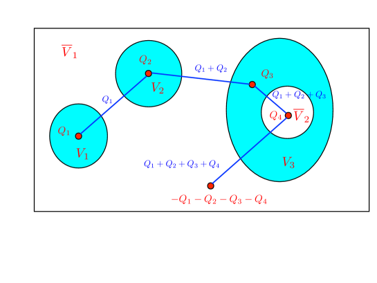
Figure 1: An example of the connection and charge distributions.

For ${}^{\forall}\{Q_{1},\cdots,Q_{\gamma}\}$ (this is also reordered), we define $\boldsymbol{k}^{Q_{1},\cdots,Q_{\gamma}}$ on a link $\ell$ as

$$k^{Q_{1},\cdots,Q_{\gamma}}_{\ell} = \left\{\begin{array}[]{ll}\sum_{i=1}^{k}Q_{i},&\mbox{ for }\ell\in\Gamma_{x_{k}x_{k+1}}\\ 0,&\mbox{otherwise}\\ \end{array}\right..$$ (123)

See Fig. 1 again as an example. A blue letter such as $Q_{1}+Q_{2}$ represents a charge on some lines, while a red letter such as $Q_{k}$ is a charge on the point $x_{k}$. Note that the net charge flowing out from the $k$-th region (some $V_{i}$ or $\bar{V}_{j}$ ) is equal to $\sum_{i=1}^{k}Q_{i}-\sum_{i=1}^{k-1}Q_{i}=Q_{k}$. It is then easy to see that the map for $\boldsymbol{k}\in\mathcal{F}_{0,\cdots,0}$ defined by

$$\varphi^{Q_{1},\cdots,Q_{\gamma}}_{0,\cdots,0}(\boldsymbol{k}):=\boldsymbol{k}+\boldsymbol{k}^{Q_{1},\cdots,Q_{\gamma}}$$ (124)

establishes an isomorphism from $\mathcal{F}_{0,\cdots,0}$ to $\mathcal{F}_{Q_{1},\cdots,Q_{\gamma}}$. This proves the number of $\mathcal{F}_{Q_{1},\cdots,Q_{\gamma}}$ is independent of $Q_{1},\cdots,Q_{\gamma}$.

A number of possible charge distribution $\left\{Q_{1},Q_{2},\cdots,Q_{\gamma}\right\}$ is $N^{\gamma}=N^{n+m-1}$. Therefore, for any charge distributions $\{q(x)\}_{x\in\mathcal{S}}$ including $\{q(x)\}_{x\in\mathcal{S}}=\{0\}_{x\in\mathcal{S}}$, the total number of the admissible $\boldsymbol{f}$ is $N^{|\partial V|-(n+m-1)}$.

Appendix B Entanglement entropy for non-abelian gauge theories

B.1 About the Hilbert space on a link

We generalize the formulation of the $Z_{n}$ case to non-abelian gauge theories. We take a group $G$ which we assume to be a compact group. We define the momentum operator $L_{\ell}(g)$ and the position operator $U^{\pi}_{\ell}$ via

$$\langle U|L_{\ell}(g)|\Psi\rangle=\Psi(g^{-1}U),\ \ \ \langle U|(U^{\pi}_{\ell})^{\alpha}{}_{\beta}|\Psi\rangle=\pi(U)^{\alpha}{}_{\beta}\Psi(U)$$ (125)

where $g\in G$ and $\pi$ is a representation of $G$. If we inverse the direction of link $\ell$, the operator $L_{\ell^{T}}(g)$ and $U_{\ell^{T}}^{\pi}$ is defined as follows:

$$\langle U|L_{\ell^{T}}(g)|\Psi\rangle=\Psi(Ug),\ \ \ \langle U|(U_{\ell^{T}}^{\pi})^{\alpha}{}_{\beta}|\Psi\rangle=\pi(U^{-1})^{\alpha}{}_{\beta}\Psi(U)=(\pi(U)^{*})_{\beta}{}^{\alpha}\Psi(U)$$ (126)

It is known that the $L^{2}$ space on a group $G$ (square integrable functions over $G$) decomposes to the direct sum of $\pi^{\dagger}\boxtimes\pi$ which is a irreducible representation of $G\times G$ as followsCMS1995 :

$$L^{2}(G)\simeq\bigoplus_{\pi\in\text{Irr}(G)}V_{\pi}^{\dagger}\otimes V_{\pi},$$ (127)

where we denote $\pi$ as an (unitary) irreducible representation of $G$ and $\text{Irr}(G)$ as the set of irreducible representation and $\pi^{\dagger}(g)={}^{t}\pi(g^{-1})$ is the dual representation. The meaning of (127) will become clear below.

We first consider the basic state $|\pi^{\alpha}{}_{\beta}\rangle$ defined via

$$\langle U|\pi^{\alpha}{}_{\beta}\rangle=\pi^{\dagger}(U)_{\beta}{}^{\alpha},$$ (128)

with which we can explicitly write the action of $L_{\ell}(g)$ as

$$\langle U|L_{\ell}(g)|\pi^{\alpha}{}_{\beta}\rangle = \pi^{\dagger}(g^{-1}U)_{\beta}{}^{\alpha}=\pi(U^{-1}g)^{\alpha}{}_{\beta}=\pi(g)^{\gamma}{}_{\beta}\langle U|\pi^{\alpha}{}_{\gamma}\rangle.$$ (129)

Therefore we have

$$L_{\ell}(g)|\pi^{\alpha}{}_{\beta}\rangle = |\pi^{\alpha}{}_{\gamma}\rangle\pi(g)^{\gamma}{}_{\beta},$$ (130)

$$L_{\ell^{T}}(g)|\pi^{\alpha}{}_{\beta}\rangle = \pi(g^{-1})^{\alpha}{}_{\gamma}|\pi^{\gamma}{}_{\beta}\rangle.$$ (131)

The dual vector of $|\pi^{\alpha}{}_{\beta}\rangle$is given by $(|\pi^{\alpha}{}_{\beta}\rangle)^{\dagger}=\langle\pi^{\beta}{}_{\alpha}|$, and the projection operator to the subspace $\pi^{\dagger}\boxtimes\pi$ is given by

$$P_{\pi}=\dim V_{\pi}\sum_{\alpha,\beta}|\pi^{\alpha}{}_{\beta}\rangle\langle\pi^{\beta}{}_{\alpha}|.$$ (132)

The factor $\dim V_{\pi}$ is needed here since the normalization of vector$|\pi^{\alpha}{}_{\beta}\rangle$ is given by

$$\langle\pi^{\alpha}{}_{\beta}|\pi^{\gamma}{}_{\delta}\rangle=\int dU\ \pi^{\alpha}{}_{\beta}(U)\pi^{\gamma}{}_{\delta}(U^{-1})=\frac{\delta^{\alpha}{}_{\delta}\delta^{\gamma}{}_{\beta}}{\dim V_{\pi}}$$ (133)

By the projection (132), the meaning of (127) becomes clear.

B.2 Gauge invariant states

In the lattice gauge theory, the total Hilbert space $\mathcal{H}_{0}$ is $\bigotimes_{l}(L^{2}(G))_{l}$. The physical Hilbert space $\mathcal{H}$ as the subspace of $\mathcal{H}_{0}$ is consist of gauge invariant states, which satisfy

$$G_{x}^{g}|\Psi\rangle=|\Psi\rangle,\qquad G_{x}^{g}:=\mathop{\prod_{y\in\mathcal{S}}}_{\mbox{s.t. }\ell=(x,y)\in\mathcal{L}}L_{\ell}(g),$$ (134)

at ${}^{\forall}x\in\mathcal{S}$. The basis state in $\mathcal{H}_{0}$ is written in general as

$$|\boldsymbol{\pi}^{\boldsymbol{\alpha}}{}_{\boldsymbol{\beta}}\rangle := \bigotimes_{\ell\in\mathcal{L}}|(\pi_{\ell})^{\alpha_{\ell}}{}_{\beta_{\ell}}\rangle$$ (135)

where $\pi_{\ell}$ indicates an irreducible representation of $G$ on a link $\ell$.

Unlike the $Z_{N}$ gauge theories, it is not so easy to write gauge invariant conditions for the state in (135). Let us consider the one dimensional case as a simplest example. In this case, the nontrivial part of the gauge invariant condition at $x$ becomes

$$|\pi^{\alpha_{1}}{}_{\gamma_{1}}\rangle_{\ell_{1}}\ \pi(g)^{\gamma_{1}}{}_{\beta_{1}}\otimes\pi^{\prime}(g^{-1})^{\alpha_{2}}{}_{\gamma_{2}}\ |\pi^{\prime}\,{}^{\gamma_{2}}{}_{\beta_{2}}\rangle_{\ell_{2}}=|\pi^{\alpha_{1}}{}_{\beta_{1}}\rangle_{\ell_{1}}\otimes|\pi^{\prime}\,{}^{\alpha_{2}}{}_{\beta_{2}}\rangle_{\ell_{2}}$$ (136)

where $\ell_{1}=(x-1,x)=(x,x-1)^{T}$ and $\ell_{2}=(x,x+1)$. Integrating this equation over $g$ with $\int dg=1$, we find that a gauge invariant state at $x$ has a form as

$$\frac{1}{\dim V_{\pi}}|\pi^{\alpha}{}_{\gamma}\rangle_{\ell_{1}}\otimes|\pi^{\gamma}{}_{\beta}\rangle_{\ell_{2}},$$ (137)

where two irreducible representations on $\ell_{1}$ and $\ell_{2}$ must be equal.

In higher dimensions, however, the condition becomes more complicated. On a $d$-dimensional hyper-cubic lattice, the gauge invariant condition at $x$ reads

$$\int dg\prod_{\mu=1}^{d}|\pi_{\mu}{}^{\alpha_{\mu}}{}_{\gamma_{\mu}}\rangle_{\ell_{\mu}}\ \pi_{\mu}(g)^{\gamma_{\mu}}{}_{\beta_{\mu}}\otimes\pi_{\bar{\mu}}(g^{-1})^{\alpha_{\bar{\mu}}}{}_{\gamma_{\bar{\mu}}}\ |\pi_{\bar{\mu}}\,{}^{\gamma_{\bar{\mu}}}{}_{\beta_{\bar{\mu}}}\rangle_{\ell_{\bar{\mu}}} = \prod_{\mu}|\pi_{\mu}{}^{\alpha_{\mu}}{}_{\beta_{\mu}}\rangle_{\ell_{\mu}}\otimes|\pi_{\bar{\mu}}\,{}^{\alpha_{\bar{\mu}}}{}_{\beta_{\bar{\mu}}}\rangle_{\ell_{\bar{\mu}}},$$

where $\ell_{\mu}=(x,x+\mu)$ and $\ell_{\bar{\mu}}=(x,x-\mu)$. This implies that a product of $2d$ irreducible representations of $\pi_{\mu}$ and $\pi_{\bar{\mu}}$ must contain the trivial representation. For example, in the case of SU(2) gauge group at $d=2$, 4 non-negative integers $k_{1,2,3,4}$, which are numbers of boxes in the SU(2) Young tableaux and specify irreducible representations of SU(2), must satisfy

$$\{|k_{1}-k_{2}|,\cdots,k_{1}+k_{2}\}\cap\{|k_{3}-k_{4}|,\cdots,k_{3}+k_{4}\}\not=\emptyset.$$

For general gauge groups in higher dimension, it is hard to find a simple condition for (LABEL:e:general_condition).

B.3 Examples

As was seen in the previous subsection, it is not so easy to construct general gauge invariant states in higher dimensions. Therefore, in this subsection, we consider two examples at $d=1$.

B.3.1 One dimensional topological state with periodic boundary condition

Assume that there are $N$ links on a circle(i.e. the periodic boundary condition). In this boundary condition, similar results are obtained by DonnellyDon in the theories defined on the continuum space. The physical Hilbert space is given by the gauge invariant functions. From the analysis in the previous subsection, the basis are given by the characters of irreducible representations as

$$|\psi\rangle=\sum_{\pi\in\text{Irr }(G)}\psi(\pi)|\pi\rangle,\ \ \ |\psi\rangle\in\mathcal{H}$$ (139)

$$|\pi\rangle=|\pi^{\alpha_{1}}{}_{\alpha_{2}}\rangle\otimes|\pi^{\alpha_{2}}{}_{\alpha_{3}}\rangle\otimes\cdots\otimes|\pi^{\alpha_{N}}{}_{\alpha_{1}}\rangle,\qquad\langle\pi|\pi\rangle=1.$$ (140)

The value of $|\pi\rangle$ at $|U_{1},\cdots,U_{N}\rangle=|U_{1}\rangle\otimes\cdots\otimes|U_{N}\rangle$ becomes as follows.

$$\langle U_{1},\cdots,U_{N}|\pi\rangle = \pi^{\dagger}(U_{1})_{\alpha_{2}}{}^{\alpha_{1}}\pi^{\dagger}(U_{2})_{\alpha_{3}}{}^{\alpha_{2}}\cdots\pi^{\dagger}(U_{N})_{\alpha_{1}}{}^{\alpha_{N}}$$ (141)

$$= \text{\text{tr}}(\pi^{\dagger}(U_{N}\cdots U_{1})).$$

As we have done in the abelian cases, to divide the physical Hilbert space into the tensor product of Hilbert spaces on the region $V$ and $\bar{V}$, we embed the physical Hilbert space $\mathcal{H}$ into a larger Hilbert space $\mathcal{H}^{\prime}$ where

$$\mathcal{H}^{\prime} = \bigoplus_{\pi,\pi^{\prime}}\bigoplus_{\boldsymbol{m}{\alpha},\boldsymbol{m}{\beta},\boldsymbol{m}{\alpha}^{\prime}\boldsymbol{m}{\beta}^{\prime}}\mathcal{H}_{V}^{(\pi)\boldsymbol{m}{\alpha}}{}_{\boldsymbol{m}{\beta}}\otimes\mathcal{H}_{\bar{V}}^{(\pi^{\prime})\boldsymbol{m}{\beta}^{\prime}}{}_{\boldsymbol{m}{\alpha}^{\prime}}.$$ (142)

Here $\boldsymbol{m}{\alpha}=(\alpha_{1},\cdots,\alpha_{M}),\boldsymbol{m}{\beta}=(\beta_{1},\cdots,\beta_{M})$ are labels of boundaries when the subsystem $V$ is consist of $M$ intervals and $\boldsymbol{m}{\alpha^{\prime}},\boldsymbol{m}{\beta^{\prime}}$ are the corresponding ones in $\bar{V}$. Then we trace over $\mathcal{H}_{\bar{V}}^{({\pi})\boldsymbol{m}{\beta}}{}_{\boldsymbol{m}{\alpha}}$, regarding the physical wave function $|\psi\rangle$ as an element of $\mathcal{H}^{\prime}$.

As the simplest case, we consider $V$ (and $\bar{V}$) is an interval. In this case, the basic is written as

$$|\pi\rangle=(\dim V_{\pi})^{-1}\times\sum_{\alpha,\beta}\sqrt{\dim V_{\pi}}|\pi_{V}^{\alpha}{}_{\beta}\rangle\otimes\sqrt{\dim V_{\pi}}|\pi_{\bar{V}}^{\beta}{}_{\alpha}\rangle.$$ (143)

The reduced density matrix for physical wave function (139) is given by

$$\rho_{V}=\sum_{\pi\in\text{Irr}(G)}p(\pi)(\dim V_{\pi})^{-2}\sum_{\alpha,\beta}(\sqrt{\dim V_{\pi}}|\pi_{V}^{\alpha}{}_{\beta}\rangle)(\sqrt{\dim V_{\pi}}\langle\pi_{V}^{\beta}{}_{\alpha}|)$$ (144)

where $p(\pi)=|\psi(\pi)|^{2}$. Its entanglement entropy is given by

$$S_{V} = -\sum_{\pi\in\text{Irr}(G),\alpha,\beta}p(\pi)(\dim V_{\pi})^{-2}\log(p(\pi)(\dim V_{\pi})^{-2})$$ (145)

$$= \sum_{\pi\in\text{Irr}(G)}p(\pi)(-\log p(\pi)+2\log\dim V_{\pi})$$

Using the above result, we compute an entanglement entropy of the topological state in finite non-abelian group $G$. The topological state is given by

$$|\text{topo}\rangle=\frac{1}{\sqrt{|G|^{2N+1}}}\sum_{g_{i}\in G}|g_{1}^{-1}g_{N}\rangle\otimes|g_{2}^{-1}g_{1}\rangle\otimes\cdots\otimes|g_{N}^{-1}g_{N-1}\rangle,$$ (146)

where $|G|$ is the number of the element of $G$, and states satisfy $\langle g|h\rangle=|G|\delta_{g,h}$. Here $|\text{topo}\rangle$ is written as the element of $\mathcal{H}_{0}$, though it is gauge invariant, and the coefficient $\psi(\pi)$ is given by

$$\psi(\pi)=\langle\pi|\text{topo}\rangle=\frac{\dim V_{\pi}}{\sqrt{|G|}},$$ (147)

which leads to $p(\pi)=(\dim V_{\pi})^{2}/|G|$. Thus the entanglement entropy is calculated as

$$S_{V}=\sum_{\pi\in\text{Irr}(G)}\frac{(\dim V_{\pi})^{2}}{|G|}\Big{(}-\log\frac{(\dim V_{\pi})^{2}}{|G|}+2\log\dim V_{\pi}\Big{)}=\log|G|,$$ (148)

where we use the identity $\sum_{\pi\in\text{Irr}(G)}(\dim V_{\pi})^{2}=|G|$. This result agrees with (92) for the $Z_{N}$ gauge theories

B.3.2 One dimensional topological state with open boundary condition

Next we consider the case with open boundary condition. From the gauge invariance of the bulk, physical wave functions are given by a linear combination of functions on $G$ as

$$|\psi\rangle = \sum_{\pi\in\text{Irr}(G),\alpha,\beta}\psi(\pi)_{\alpha}{}^{\beta}\sqrt{\dim V_{\pi}}|\pi_{\rm tot}{}^{\alpha}{}_{\beta}\rangle\ \ \ |\psi\rangle\in\mathcal{H}$$ (149)

$$|\pi_{\rm tot}{}^{\alpha}{}_{\beta}\rangle = |\pi^{\alpha}{}_{\alpha_{1}}\rangle\otimes|\pi^{\alpha_{1}}{}_{\alpha_{2}}\rangle\otimes\cdots\otimes|\pi^{\alpha_{N-1}}{}_{\beta}\rangle$$ (150)

The value at $|U_{1},\cdots,U_{N}\rangle$ becomes as follows.

$$\langle U_{1},\cdots,U_{N}|\pi_{\rm tot}{}^{\alpha}{}_{\beta}\rangle = \pi^{\dagger}(U_{1})_{\alpha_{1}}{}^{\alpha}\pi^{\dagger}(U_{2})_{\alpha_{2}}{}^{\alpha_{1}}\cdots\pi^{\dagger}(U_{N})_{\beta}{}^{\alpha_{N-1}}$$ (151)

$$= \pi^{\dagger}(U_{N}\cdots U_{1})_{\beta}{}^{\alpha}.$$

This confirms that the physical Hilbert space is spanned by the functions on the group $G$.

For example, we consider $V$ is an interval in the middle. In this case, the basis is given by

$$\sqrt{\dim V_{\pi}}|\pi_{\rm tot}{}^{\alpha}{}_{\beta}\rangle=(\dim V_{\pi})^{-1}\sum_{\gamma,\delta}\sqrt{\dim V_{\pi}}|\pi_{\bar{V}}^{\alpha}{}_{\gamma}\rangle\otimes\sqrt{\dim V_{\pi}}|\pi_{V}^{\gamma}{}_{\delta}\rangle\otimes\sqrt{\dim V_{\pi}}|\pi_{\bar{V}}^{\delta}{}_{\beta}\rangle.$$ (152)

From the decomposition, we find the reduced density matrix is given by

$$\rho_{V}=\sum_{\pi}p(\pi)(\dim V_{\pi})^{-2}\sum_{\gamma,\delta}(\sqrt{\dim V_{\pi}}|\pi_{V}^{\gamma}{}_{\delta}\rangle)(\sqrt{\dim V_{\pi}}\langle\pi_{V}^{\delta}{}_{\gamma}|)$$ (153)

where $p(\pi)=\sum\psi(\pi)_{\alpha}{}^{\beta}\psi^{*}(\pi)_{\beta}{}^{\alpha}$. The expression of the reduced density matrix is the same with the case of periodic boundary condition (144), so that the entanglement entropy is given by the same formula (145) .

The topological state with open boundary condition is given by

$$|\text{topo}\rangle=\frac{1}{\sqrt{|G|^{2N-1}}}\sum_{g_{i}\in G}|g_{1}^{-1}\rangle\otimes|g_{2}^{-1}g_{1}\rangle\otimes\cdots\otimes|g_{N-1}^{-1}g_{N-2}\rangle\otimes|g_{N-1}\rangle.$$ (154)

Thus $\sqrt{\dim V_{\pi}}|\pi_{\rm tot}{}^{\alpha}{}_{\beta}\rangle$ component is obtained as

$$\psi_{\alpha}{}^{\beta}(\pi)=\sqrt{\dim V_{\pi}}\langle\pi^{\beta}{}_{\alpha}|\text{topo}\rangle=\sqrt{\frac{\dim V_{\pi}}{|G|}}\delta_{\alpha}{}^{\beta},$$ (155)

and $p(\pi)$ becomes

$$p(\pi)=\frac{(\dim V_{\pi})^{2}}{|G|},$$ (156)

which is identical to the result with the periodic boundary condition case. We thus obtain the same result also for the entanglement entropy as

$$S_{V}=\log|G|.$$ (157)

References

- (1) S. Ryu and T. Takayanagi, “Aspects of Holographic Entanglement Entropy,” JHEP 0608, 045 (2006) [hep-th/0605073].
- (2) S. Ryu and T. Takayanagi, “Holographic derivation of entanglement entropy from AdS/CFT,” Phys. Rev. Lett. 96, 181602 (2006) [hep-th/0603001]; V. E. Hubeny, M. Rangamani and T. Takayanagi, “A Covariant holographic entanglement entropy proposal,” JHEP 0707 (2007) 062 [arXiv:0705.0016 [hep-th]]; T. Nishioka, S. Ryu and T. Takayanagi, “Holographic Entanglement Entropy: An Overview,” J. Phys. A 42 (2009) 504008; T. Takayanagi, “Entanglement Entropy from a Holographic Viewpoint,” Class. Quant. Grav. 29 (2012) 153001 [arXiv:1204.2450 [gr-qc]].
- (3) B. Swingle, “Entanglement Renormalization and Holography,” Phys. Rev. D 86, 065007 (2012) [arXiv:0905.1317 [cond-mat.str-el]].
- (4) B. Swingle, “Constructing holographic spacetimes using entanglement renormalization,” arXiv:hep-th/1209.3304
- (5) M. Van Raamsdonk, “Building up spacetime with quantum entanglement,” Gen. Rel. Grav. 42, 2323 (2010) [Int. J. Mod. Phys. D 19, 2429 (2010)] [arXiv:1005.3035 [hep-th]]; M. Van Raamsdonk, “Comments on quantum gravity and entanglement,” arXiv:0907.2939 [hep-th].
- (6) M. Nozaki, S. Ryu and T. Takayanagi, “Holographic Geometry of Entanglement Renormalization in Quantum Field Theories,” JHEP 1210, 193 (2012) [arXiv:1208.3469 [hep-th]]; A. Mollabashi, M. Nozaki, S. Ryu and T. Takayanagi, “Holographic Geometry of cMERA for Quantum Quenches and Finite Temperature,” JHEP 1403, 098 (2014) [arXiv:1311.6095 [hep-th]]; M. Miyaji, S. Ryu, T. Takayanagi and X. Wen, “Boundary States as Holographic Duals of Trivial Spacetimes,” arXiv:hep-th/1412.6226
- (7) M. Nozaki, T. Numasawa, A. Prudenziati and T. Takayanagi, “Dynamics of Entanglement Entropy from Einstein Equation,” Phys. Rev. D 88, 026012 (2013) [arXiv:1304.7100 [hep-th]]; J. Bhattacharya and T. Takayanagi, “Entropic Counterpart of Perturbative Einstein Equation,” JHEP 1310, 219 (2013) [arXiv:1308.3792 [hep-th]].
- (8) T. Faulkner, M. Guica, T. Hartman, R. C. Myers and M. Van Raamsdonk, “Gravitation from Entanglement in Holographic CFTs,” JHEP 1403, 051 (2014) [arXiv:1312.7856 [hep-th]]; N. Lashkari, M. B. McDermott and M. Van Raamsdonk, “Gravitational Dynamics From Entanglement Thermodynamics,” JHEP 1404, 195 (2014) [arXiv:1308.3716 [hep-th]].
- (9) M. Levin and X. G. Wen, “Detecting Topological Order in a Ground State Wave Function,” Phys. Rev. Lett. 96, 110405 (2006) [arXiv:cond-mat/0510613].
- (10) A. Kitaev and J. Preskill, “Topological entanglement entropy,” Phys. Rev. Lett. 96, 110404 (2006) [arXiv:hep-th/0510092].
- (11) B. Hsu, M. Mulligan, E. Fradkin and E.A. Kim, “Universal entanglement entropy in 2D conformal quantum critical points,” Phys. Rev. B 79, 115421 (2009) [arXiv:0812.0203].
- (12) H. Li and F. D. M. Haldane, “Entanglement Spectrum as a Generalization of Entanglement Entropy: Identification of Topological Order in Non-Abelian Fractional Quantum Hall Effect States,” Phys. Rev. Lett. 101, 010504 (2008) [arXiv:0805.0332 [cond-mat.mes-hall]].
- (13) S. T. Flammia, A. Hamma, T. L. Hughes, and X.-G. Wen, “Topological Entanglement Renyi Entropy and Reduced Density Matrix Structure,” Phys. Rev. Lett. 103, 261601 (2009) [arXiv:0909.3305 [cond-mat.str-el]].
- (14) M. B. Hastings, I. Gonzalez, A. B. Kallin, and R. G. Melko, “Measuring Renyi Entanglement Entropy in Quantum Monte Carlo Simulations,” Phys. Rev. Lett. 104, 157201 (2010) [arXiv:1001.2335 [cond-mat.str-el]].
- (15) L. Susskind and J. Uglum, “Black hole entropy in canonical quantum gravity and superstring theory,” Phys. Rev. D 50, 2700 (1994) [hep-th/9401070].
- (16) D. N. Kabat, “Black hole entropy and entropy of entanglement,” Nucl. Phys. B 453, 281 (1995) [hep-th/9503016].
- (17) D. N. Kabat and M. J. Strassler, “A Comment on entropy and area,” Phys. Lett. B 329, 46 (1994) [hep-th/9401125].
- (18) N. Shiba, “Entanglement Entropy of Two Black Holes and Entanglement Entropic Force,” Phys. Rev. D 83, 065002 (2011) [arXiv:1011.3760 [hep-th]].
- (19) N. Shiba, “Entanglement Entropy of Two Spheres,” JHEP 1207, 100 (2012) [arXiv:1201.4865 [hep-th]].
- (20) T. Nishioka and T. Takayanagi, “AdS Bubbles, Entropy and Closed String Tachyons,” JHEP 0701, 090 (2007) [hep-th/0611035].
- (21) I. R. Klebanov, D. Kutasov and A. Murugan, “Entanglement as a probe of confinement,” Nucl. Phys. B 796, 274 (2008) [arXiv:0709.2140 [hep-th]].
- (22) A. Lewkowycz, “Holographic Entanglement Entropy and Confinement,” JHEP 1205, 032 (2012) [arXiv:1204.0588 [hep-th]].
- (23) H. Casini, M. Huerta and J. A. Rosabal, “Remarks on entanglement entropy for gauge fields”, arXiv:hep-th/1312.1183.
- (24) D. Radievi, “Note on Entanglement in Abelian Gauge Theories”, arXiv:hep-th/1404.1391.
- (25) P. V. Buividovich and M. I. Polikarpov, “Entanglement entropy in gauge theories and holographic principle for electric strings,” Phys, Lett. B670, 141 (2008).
- (26) W. Donnelly, “Decomposition of entanglement entropy in lattice gauge theories”, Phys. Rev. D85, 085004 (2012).
- (27) W. Donnelly, “Entanglement entropy and nonabelian gauge symmetry”, arXiv:hep-th/1406.7304.
- (28) M. Creutz, “Gauge fixing, the transfer matrix and confinement on a lattice”, Phys. Rev. D15, 1128 (1977).
- (29) M. Lüsher, “Construction of a selfadjoint, strictly positive transfer matrix for Euclidean lattice gauge theories,” Comm. Math. Phys. 54, 283(1977).
- (30) See, for example: M. A. Nielsen and I. L. Chuang, “Quantum computation and quantum information,” Cambridge University Press, Cambridge, 2000.
- (31) A. Hamma, R. Ionicioiu, P. Zanardi, “Ground state entanglement and geometric entropy in the Kitaev’s model,” Phys. Lett. A 337, 22 (2005).
- (32) A. Hamma, R. Ionicioiu, P. Zanardi, “Biparticle entanglement and entropic boundary law in lattice spin systems,” Phys. Rev. A 71, 022315 (2005).
- (33) T. Nishioka, “Relevant Perturbation of Entanglement Entropy and Stationarity,” Phys. Rev. D 90, no. 4, 045006 (2014) [arXiv:1405.3650 [hep-th]].
- (34) V. Rosenhaus and M. Smolkin, “Entanglement Entropy: A Perturbative Calculation,” JHEP 1412, 179 (2014) [arXiv:1403.3733 [hep-th]].
- (35) V. Rosenhaus and M. Smolkin, “Entanglement Entropy for Relevant and Geometric Perturbations,” arXiv:hep-th/1410.6530.
- (36) K. W. Huang, “Central Charge and Entangled Gauge Fields,” arXiv:1412.2730 [hep-th].
- (37) P. V. Buividovich and M. I. Polikarpov, “Numerical study of entanglement entropy in SU(2) lattice gauge theory,” Nucl. Phys. B 802, 458 (2008) [arXiv:0802.4247 [hep-lat]].
- (38) Y. Nakagawa, A. Nakamura, S. Motoki and V. I. Zakharov, “Entanglement entropy of SU(3) Yang-Mills theory”, PoS LAT 2009, 188 (2009) [arXiv:0911.2596 [hep-lat]].
- (39) Y. Nakagawa, A. Nakamura, S. Motoki, V.I. Zakharov, “Quantum entanglement in SU(3) lattice Yang-Mills theory at zero and finite temperatures,” PoS Lattice2010, 281 (2010).
- (40) S. Ghosh, R.M. Soni, S.P. Trivedi, “On the entanglement entropy for gauge theories,” arXiv:hep-th/1501.02593.
- (41) L. Y. Hung and Y. Wan, “Revisiting Entanglement Entropy of Lattice Gauge Theories,” arXiv:hep-th/1501.04389.
- (42) R. W. Carter, I. G. MacDonald and G. B. Segal, in “Lectures on Lie groups and Lie algebras,” Cambridge University Press, 1995