Abstract

Additive regression trees are flexible non-parametric models and popular off-the-shelf tools for real-world non-linear regression. In application domains, such as bioinformatics, where there is also demand for probabilistic predictions with measures of uncertainty, the Bayesian additive regression trees (BART) model, introduced by Chipman et al. (2010), is increasingly popular. As data sets have grown in size, however, the standard Metropolis–Hastings algorithms used to perform inference in BART are proving inadequate. In particular, these Markov chains make local changes to the trees and suffer from slow mixing when the data are high-dimensional or the best-fitting trees are more than a few layers deep. We present a novel sampler for BART based on the Particle Gibbs (PG) algorithm (Andrieu et al., 2010) and a top-down particle filtering algorithm for Bayesian decision trees (Lakshminarayanan et al., 2013). Rather than making local changes to individual trees, the PG sampler proposes a complete tree to fit the residual. Experiments show that the PG sampler outperforms existing samplers in many settings.

1 Introduction

Ensembles of regression trees are at the heart of many state-of-the-art approaches for nonparametric regression (Caruana and Niculescu-Mizil, 2006), and can be broadly classified into two families: randomized independent regression trees, wherein the trees are grown independently and predictions are averaged to reduce variance, and additive regression trees, wherein each tree fits the residual not explained by the remainder of the trees. In the former category are bagged decision trees (Breiman, 1996), random forests (Breiman, 2001), extremely randomized trees (Geurts et al., 2006), and many others, while additive regression trees can be further categorized into those that are fit in a serial fashion, like gradient boosted regression trees (Friedman, 2001), and those fit in an iterative fashion, like Bayesian additive regression trees (BART) (Chipman et al., 2010) and additive groves (Sorokina et al., 2007).

Among additive approaches, BART is extremely popular and has been successfully applied to a wide variety of problems including protein-DNA binding, credit risk modeling, automatic phishing/spam detection, and drug discovery (Chipman et al., 2010). Additive regression trees must be regularized to avoid overfitting (Friedman, 2002): in BART, over-fitting is controlled by a prior distribution preferring simpler tree structures and non-extreme predictions at leaves. At the same time, the posterior distribution underlying BART delivers a variety of inferential quantities beyond predictions, including credible intervals for those predictions as well as a measures of variable importance. At the same time, BART has been shown to achieve predictive performance comparable to random forests, boosted regression trees, support vector machines, and neural networks (Chipman et al., 2010).

The standard inference algorithm for BART is an iterative Bayesian backfitting Markov Chain Monte Carlo (MCMC) algorithm (Hastie et al., 2000). In particular, the MCMC algorithm introduced by Chipman et al. (2010) proposes local changes to individual trees. This sampler can be computationally expensive for large datasets, and so recent work on scaling BART to large datasets (Pratola et al., 2013) considers using only a subset of the moves proposed by Chipman et al. (2010). However, this smaller collection of moves has been observed to lead to poor mixing (Pratola, 2013) which in turn produces an inaccurate approximation to the posterior distribution. While a poorly mixing Markov chain might produce a reasonable prediction in terms of mean squared error, BART is often used in scenarios where its users rely on posterior quantities, and so there is a need for computationally efficient samplers that mix well across a range of hyper-parameter settings.

In this work, we describe a novel sampler for BART based on (1) the Particle Gibbs (PG) framework proposed by Andrieu et al. (2010) and (2) the top-down sequential Monte Carlo algorithm for Bayesian decision trees proposed by Lakshminarayanan et al. (2013). Loosely speaking, PG is the particle version of the Gibbs sampler where proposals from the exact conditional distributions are replaced by conditional versions of a sequential Monte Carlo (SMC) algorithm. The complete sampler follows the Bayesian backfitting MCMC framework for BART proposed by Chipman et al. (2010); the key difference is that trees are sampled using PG instead of the local proposals used by Chipman et al. (2010). Our sampler, which we refer to as PG-BART, approximately samples complete trees from the conditional distribution over a tree fitting the residual. As the experiments bear out, the PG-BART sampler explores the posterior distribution more efficiently than samplers based on local moves. Of course, one could easily consider non-local moves in a Metropolis–Hastings (MH) scheme by proposing complete trees from the tree prior, however these moves would be rejected, leading to slow mixing, in high-dimensional and large data settings. The PG-BART sampler succeeds not only because non-local moves are considered, but because those non-local moves have high posterior probability. Another advantage of the PG sampler is that it only requires one to be able to sample from the prior and does not require evaluation of tree prior in the acceptance ratio unlike (local) MH—hence PG can be computationally efficient in situations where the tree prior is expensive (or impossible) to compute, but relatively easier to sample from.

The paper is organized as follows: in section 2, we review the BART model; in section 3, we review the MCMC framework proposed by Chipman et al. (2010) and describe the PG sampler in detail. In section 4, we present experiments that compare the PG sampler to existing samplers for BART.

2 Model and notation

In this section, we briefly review decision trees and the BART model. We refer the reader to the paper of Chipman et al. (2010) for further details about the model. Our notation closely follows their’s, but also borrows from Lakshminarayanan et al. (2013).

2.1 Problem setup

We assume that the training data consist of $N$ i.i.d. samples $\bm{X}=\{\bm{x}_{n}\}_{n=1}^{N}$, where $\bm{x}_{n}\in\mathbb{R}^{D}$, along with corresponding labels ${Y}=\{y_{n}\}_{n=1}^{N}$, where $y_{n}\in\mathbb{R}$. We focus only on the regression task in this paper, although the PG sampler can also be used for classification by building on the work of Chipman et al. (2010) and Zhang and Härdle (2010).

2.2 Decision tree

For our purposes, a decision tree is a hierarchical binary partitioning of the input space with axis-aligned splits. The structure of the decision tree is a finite, rooted, strictly binary tree $\mathsf{T}$, i.e., a finite collection of nodes such that 1) every node $\eta$ has exactly one parent node, except for a distinguished root node $\epsilon$ which has no parent, and 2) every node $\eta$ is the parent of exactly zero or two children nodes, called the left child $\eta 0$ and the right child $\eta 1$. Denote the leaves of $\mathsf{T}$ (those nodes without children) by $\mathsf{leaves}(\mathsf{T})$. Each node of the tree $\eta\in\mathsf{T}$ is associated with a block $B_{\eta}\subset\mathbb{R}^{D}$ of the input space as follows: At the root, we have $B_{\epsilon}=\mathbb{R}^{D}$, while each internal node $\eta\in\mathsf{T}\setminus\mathsf{leaves}(\mathsf{T})$ with two children represents a split of its parent’s block into two halves, with $\kappa_{\eta}\in\{1,\dotsc,D\}$ denoting the dimension of the split, and $\tau_{\eta}$ denoting the location of the split. In particular,

$$B_{\eta 0} =B_{\eta}\cap\{\bm{z}\in\mathbb{R}^{D}:z_{\kappa_{\eta}}\leq\tau_{\eta}\}\text{ and }$$

$$B_{\eta 1} =B_{\eta}\cap\{\bm{z}\in\mathbb{R}^{D}:z_{\kappa_{\eta}}>\tau_{\eta}\}.$$ (1)

We call the tuple $\mathcal{T}=(\mathsf{T},\bm{\kappa},\bm{\tau})$ a decision tree. Note that the blocks associated with the leaves of the tree form a partition of $\mathbb{R}^{D}$.

A decision tree used for regression is referred to as a regression tree. In a regression tree, each leaf node $\eta\in\mathsf{leaves}(\mathsf{T})$ is associated with a real-valued parameter $\mu_{\eta}\in\mathbb{R}$. Let $\bm{\mu}=\{\mu_{\eta}\}_{\eta\in\mathsf{leaves}(\mathsf{T})}$ denote the collection of all parameters. Given a tree $\mathcal{T}$ and a data point $\bm{x}$, let $\mathsf{leaf}_{\mathcal{T}}(\bm{x})$ be the unique leaf node $\eta\in\mathsf{leaves}(\mathsf{T})$ such that $\bm{x}\in B_{\eta}$, and let $g(\,\cdot\,;\mathcal{T},\bm{\mu})$ be the response function associated with $\mathcal{T}$ and $\bm{\mu}$, given by

$$g(\bm{x};\mathcal{T},\bm{\mu}):=\mu_{\mathsf{leaf}_{\mathcal{T}}(\bm{x})}.$$ (2)

2.3 Likelihood specification for BART

BART is a sum-of-trees model, i.e., BART assumes that the label $y$ for an input $\bm{x}$ is generated by an additive combination of $m$ regression trees. More precisely,

$$y=\sum_{j=1}^{m}g(\bm{x};\mathcal{T}_{j},\bm{\mu}_{j})+e,$$ (3)

where $e\sim\mathcal{N}(0,\sigma^{2})$ is an independent Gaussian noise term with zero mean and variance $\sigma^{2}$. Hence, the likelihood for a training instance is

$$\ell(y|\{\mathcal{T}_{j},\bm{\mu}_{j}\}_{j=1}^{m},\sigma^{2},\bm{x})=\mathcal{N}\bigl{(}y|\sum_{j=1}^{m}g(\bm{x};\mathcal{T}_{j},\bm{\mu}_{j}),\sigma^{2}\bigr{)},$$

and the likelihood for the entire training dataset is

$$\ell({Y}|\{\mathcal{T}_{j},\bm{\mu}_{j}\}_{j=1}^{m},\sigma^{2},\bm{X})=\prod_{n}\ell(y_{n}|\{\mathcal{T}_{j},\bm{\mu}_{j}\}_{j=1}^{m},\sigma^{2},\bm{x}_{n}).$$

2.4 Prior specification for BART

The parameters of the BART model are the noise variance $\sigma^{2}$ and the regression trees $(\mathcal{T}_{j},\bm{\mu}_{j})$ for $j=1,\dotsc,m$. The conditional independencies in the prior are captured by the factorization

$$p(\{\mathcal{T}_{j},\bm{\mu}_{j}\}_{j=1}^{m},\sigma^{2}|\bm{X})=p(\sigma^{2})\prod_{j=1}^{m}p(\bm{\mu}_{j}|\mathcal{T}_{j})p(\mathcal{T}_{j}|\bm{X}).$$

The prior over decision trees $p(\mathcal{T}_{j}=\{\mathsf{T}_{j},\kappa_{j},\tau_{j}\}|\bm{X})$ can be described by the following generative process (Chipman et al., 2010; Lakshminarayanan et al., 2013): Starting with a tree comprised only of a root node $\epsilon$, the tree is grown by deciding once for every node $\eta$ whether to 1) stop and make $\eta$ a leaf, or 2) split, making $\eta$ an internal node, and add $\eta 0$ and $\eta 1$ as children. The same stop/split decision is made for the children, and their children, and so on. Let $\rho_{\eta}$ be a binary indicator variable for the event that $\eta$ is split. Then every node $\eta$ is split independently with probability

$$p(\rho_{\eta}=1)= \frac{\alpha_{s}}{(1+0pt(\eta))^{\beta_{s}}}$$

$$\times\mathds{1}[\text{valid split exists below $\eta$ in $\bm{X}$}],$$ (4)

where the indicator $\mathds{1}[...]$ forces the probability to be zero when every possible split of $\eta$ is invalid, i.e., one of the children nodes contains no training data. Informally, the hyperparameters $\alpha_{s}\in(0,1)$ and $\beta_{s}\in[0,\infty)$ control the depth and number of nodes in the tree. Higher values of $\alpha_{s}$ lead to deeper trees while higher values of $\beta_{s}$ lead to shallower trees.

In the event that a node $\eta$ is split, the dimension $\kappa_{\eta}$ and location $\tau_{\eta}$ of the split are assumed to be drawn independently from a uniform distribution over the set of all valid splits of $\eta$. The decision tree prior is thus

$$p(\mathcal{T}|\bm{X})= \prod_{\eta\in\mathsf{T}\setminus\mathsf{leaves}(\mathsf{T})}p(\rho_{\eta}=1)\,\mathcal{U}(\kappa_{\eta})\,\mathcal{U}(\tau_{\eta}|\kappa_{\eta})$$

$$\times\prod_{\eta\in\mathsf{leaves}(\mathsf{T})}p(\rho_{\eta}=0),$$ (5)

where $\mathcal{U}(\cdot)$ denotes the probability mass function of the uniform distribution over dimensions that contain at least one valid split, and $\mathcal{U}(\cdot|\kappa_{\eta})$ denotes the probability density function of the uniform distribution over valid split locations along dimension $\kappa_{\eta}$ in block $B_{\eta}$.

Given a decision tree $\mathcal{T}$, the parameters associated with its leaves are independent and identically distributed normal random variables, and so

$$p(\bm{\mu}|\mathcal{T})=\prod_{\eta\in\mathsf{leaves}(\mathsf{T})}\mathcal{N}(\mu_{\eta}|m_{\mu},\sigma_{\mu}^{2}).$$ (6)

The mean $m_{\mu}$ and variance $\sigma_{\mu}^{2}$ hyperparameters are set indirectly: Chipman et al. (2010) shift and rescale the labels $Y$ such that $y_{\min}=-0.5$ and $y_{\max}=0.5$, and set $m_{\mu}=0$ and $\sigma_{\mu}=0.5/k\sqrt{m}$, where $k>0$ is an hyperparameter. This adjustment has the effect of keeping individual node parameters $\mu_{\eta}$ small; the higher the values of $k$ and $m$, the greater the shrinkage towards the mean $m_{\mu}$.

The prior $p(\sigma^{2})$ over the noise variance is an inverse gamma distribution. The hyperparameters $\nu$ and $q$ indirectly control the shape and rate of the inverse gamma prior over $\sigma^{2}$. Chipman et al. (2010) compute an overestimate of the noise variance $\widehat{\sigma}^{2}$, e.g., using the least-squares variance or the unconditional variance of $Y$, and, for a given shape parameter $\nu$, set the rate such that $\Pr(\sigma\leq\widehat{\sigma})=q$, i.e., the $q$th quantile of the prior over $\sigma$ is located at $\widehat{\sigma}$.

Chipman et al. (2010) recommend the default values: $\nu=3,q=0.9,k=2,m=200$ and $\alpha_{s}=0.95,\beta_{s}=2.0$. Unless otherwise specified, we use this default hyperparameter setting in our experiments.

2.5 Sequential generative process for trees

Lakshminarayanan et al. (2013) present a sequential generative process for the tree prior $p(\mathcal{T}|\bm{X})$, where a tree $\mathcal{T}$ is generated by starting from an empty tree $\mathcal{T}_{(0)}$ and sampling a sequence $\mathcal{T}_{(1)},\mathcal{T}_{(2)},\dotsc$ of partial trees. This sequential representation is used as the scaffolding for their SMC algorithm. Due to space limitations, we can only briefly review the sequential process. The interested reader should refer to the paper by Lakshminarayanan et al. (2013): Let $\mathcal{T}_{(t)}=\mathsf{T}_{(t)},\bm{\kappa}_{(t)},\bm{\tau}_{(t)},E_{(t)}$ denote the partial tree at stage $t$, where $E_{(t)}$ denotes the ordered set containing the list of nodes eligible for expansion at stage $t$. At stage $t$, the generative process samples $\mathcal{T}_{(t)}$ from $\Pr_{t}(\cdot\,|\,\mathcal{T}_{(t-1)})$ as follows: the first element of $E$, say $\eta$, is popped and is stochastically assigned to be an internal node or a leaf node with probability given by (2.4). If $\eta$ is chosen to be an internal node, we sample the split dimension $\kappa_{\eta}$ and split location $\tau_{\eta}$ uniformly among the valid splits, and append $\eta 0$ and $\eta 1$ to $E$. Thus, the tree is expanded in a breadth-wise fashion and each node is visited just once. The process terminates when $E$ is empty. Figure 1 presents a cartoon of the sequential generative process.

(a) $\mathcal{T}_{(0)}$: $E_{(0)}=\{\epsilon\}$

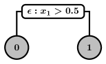
(b) $\mathcal{T}_{(1)}$: $E_{(1)}=\{0,1\}$

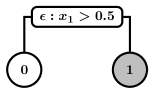
(c) $\mathcal{T}_{(2)}$: $E_{(2)}=\{1\}$

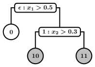
(d) $\mathcal{T}_{(3)}$: $E_{(3)}=\{10,11\}$

(e) $\mathcal{T}_{(6)}$: $E_{(6)}=\{\}$

Figure 1: Sequential generative process for decision trees: Nodes eligible for expansion are denoted by the ordered set $E$ and shaded in gray. At iteration 0, we start with the empty tree and $E=\{\epsilon\}$. At iteration 1, we pop $\epsilon$ from $E$ and assign it to be an internal node with split dimension $\kappa_{\epsilon}=1$ and split location $\tau_{\epsilon}=0.5$ and append the child nodes $0$ and $1$ to $E$. At iteration 2, we pop $0$ from $E$ and set it to a leaf node. At iteration 3, we pop $1$ from $E$ and set it to an internal node, split dimension $\kappa_{1}=2$ and threshold $\tau_{1}=0.3$ and append the child nodes $10$ and $11$ to $E$. At iterations $4$ and $5$ (not shown), we pop nodes $10$ and $11$ respectively and assign them to be leaf nodes. At iteration $6$, $E=\{\}$ and the process terminates. By arranging the random variables $\rho$ and $\kappa,\tau$ (if applicable) for each node in the order of expansion, the tree can be encoded as a sequence.

Algorithm 1 Bayesian backfitting MCMC for posterior inference in BART

1:Inputs: Training data $(\bm{X},Y)$, BART hyperparameters $(\nu,q,k,m,\alpha_{s},\beta_{s})$

2:Initialization: For all $j$, set $\mathcal{T}_{j}^{(0)}=\{\mathsf{T}_{j}^{(0)}=\{\epsilon\}$, $\bm{\tau}_{j}^{(0)}=\bm{\kappa}_{j}^{(0)}=\emptyset\}$ and sample $\bm{\mu}_{j}^{(0)}$

3:for $i=1:\mathsf{max\_iter}$ do

4:     Sample $\sigma^{2(i)}|\mathcal{T}_{1:m}^{(i-1)},\bm{\mu}_{1:m}^{(i-1)}$ $\triangleright$ sample from inverse gamma distribution

5:     for $j=1:m$ do

6:         Compute residual $R_{j}^{(i)}$ $\triangleright$ using (8)

7:         Sample $\mathcal{T}_{j}^{(i)}|R_{j}^{(i)},\sigma^{2(i)},\mathcal{T}_{j}^{(i-1)}$ $\triangleright$ using CGM, GrowPrune or PG

8:         Sample $\bm{\mu}_{j}^{(i)}|R_{j}^{(i)},\sigma^{2(i)},\mathcal{T}_{j}^{(i)}$ $\triangleright$ sample from Gaussian distribution     

3 Posterior inference for BART

In this section, we briefly review the MCMC framework proposed in (Chipman et al., 2010), discuss limitations of existing samplers and then present our PG sampler.

3.1 MCMC for BART

Given the likelihood and the prior, our goal is to compute the posterior distribution

$$p(\{\mathcal{T}_{j},\bm{\mu}_{j}\}_{j=1}^{m},\sigma^{2}|Y,\bm{X})\ \propto\qquad\qquad\qquad\qquad\quad$$

$$\quad\ell(Y|\{\mathcal{T}_{j},\bm{\mu}_{j}\}_{j=1}^{m},\sigma^{2},\bm{X})\ p(\{\mathcal{T}_{j},\bm{\mu}_{j}\}_{j=1}^{m},\sigma^{2}|\bm{X}).$$ (7)

Chipman et al. (2010) proposed a Bayesian backfitting MCMC to sample from the BART posterior. At a high level, the Bayesian backfitting MCMC is a Gibbs sampler that loops through the trees, sampling each tree $\mathcal{T}_{j}$ and associated parameters $\bm{\mu}_{j}$ conditioned on $\sigma^{2}$ and the remaining trees and their associated parameters $\{\mathcal{T}_{j^{\prime}},\bm{\mu}_{j^{\prime}}\}_{j^{\prime}\neq j}$, and samples $\sigma^{2}$ conditioned on all the trees and parameters $\{\mathcal{T}_{j},\bm{\mu}_{j}\}_{j=1}^{m}$. Let $\mathcal{T}_{j}^{(i)},\mu_{j}^{(i)},$ and $\sigma^{2(i)}$ respectively denote the values of $\mathcal{T}_{j},\mu_{j}$ and $\sigma^{2}$ at the $i^{th}$ MCMC iteration. Sampling $\sigma^{2}$ conditioned on $\{\mathcal{T}_{j},\bm{\mu}_{j}\}_{j=1}^{m}$ is straightforward due to conjugacy. To sample $\mathcal{T}_{j},\bm{\mu}_{j}$ conditioned on the other trees $\{\mathcal{T}_{j^{\prime}},\bm{\mu}_{j^{\prime}}\}_{j^{\prime}\neq j}$, we first sample $\mathcal{T}_{j}|\{\mathcal{T}_{j^{\prime}},\bm{\mu}_{j^{\prime}}\}_{j^{\prime}\neq j},\sigma^{2}$ and then sample $\bm{\mu}_{j}|\mathcal{T}_{j},\{\mathcal{T}_{j^{\prime}},\bm{\mu}_{j^{\prime}}\}_{j^{\prime}\neq j},\sigma^{2}$. (Note that $\bm{\mu}_{j}$ is integrated out while sampling $\mathcal{T}_{j}$.) More precisely, we compute the residual

$$R_{j}= \ Y-\textstyle\sum_{j^{\prime}=1,j^{\prime}\neq j}^{m}g(\bm{X};\mathcal{T}_{j^{\prime}},\mu_{j^{\prime}}).$$ (8)

Using the residual $R_{j}^{(i)}$ as the target, Chipman et al. (2010) sample $\mathcal{T}_{j}^{(i)}$ by proposing local changes to $\mathcal{T}_{j}^{(i-1)}$. Finally, $\bm{\mu}_{j}$ is sampled from a Gaussian distribution conditioned on $\mathcal{T}_{j},\{\mathcal{T}_{j^{\prime}},\bm{\mu}_{j^{\prime}}\}_{j^{\prime}\neq j},\sigma^{2}$. The procedure is summarized in Algorithm 1.

3.2 Existing samplers for BART

To sample $\mathcal{T}_{j}$, Chipman et al. (2010) use the MCMC algorithm proposed by Chipman et al. (1998). This algorithm, which we refer to as CGM. CGM is a Metropolis-within-Gibbs sampler that randomly chooses one of the following four moves: grow (which randomly chooses a leaf node and splits it further into left and right children), prune (which randomly chooses an internal node where both the children are leaf nodes and prunes the two leaf nodes, thereby making the internal node a leaf node), change (which changes the decision rule at a randomly chosen internal node), swap (which swaps the decision rules at a parent-child pair where both the parent and child are internal nodes). There are two issues with the CGM sampler: (1) the CGM sampler makes local changes to the tree, which is known to affect mixing when computing the posterior over a single decision tree (Wu et al., 2007). Chipman et al. (2010) claim that the default hyper-parameter values encourage shallower trees and hence mixing is not affected significantly. However, if one wishes to use BART on large datasets where individual trees are likely to be deeper, the CGM sampler might suffer from mixing issues. (2) The change and swap moves in CGM sampler are computationally expensive for large datasets that involve deep trees (since they involve re-computation of all likelihoods in the subtree below the top-most node affected by the proposal). For computational efficiency, Pratola et al. (2013) propose using only the grow and prune moves; we will call this the GrowPrune  sampler. However, as we illustrate in section 4, the GrowPrune  sampler can inefficiently explore the posterior in scenarios where there are multiple possible trees that explain the observations equally well. In the next section, we present a novel sampler that addresses both of these concerns.

3.3 PG sampler for BART

Recall that Chipman et al. (2010) sample $\mathcal{T}_{j}^{(i)}$ using $R_{j}^{(i)}$ as the target by proposing local changes to $\mathcal{T}_{j}^{(i-1)}$. It is natural to ask if it is possible to sample a complete tree $\mathcal{T}_{j}^{(i)}$ rather than just local changes. Indeed, this is possible by marrying the sequential representation of the tree proposed by Lakshminarayanan et al. (2013) (see section 2.5) with the Particle Markov Chain Monte Carlo (PMCMC) framework (Andrieu et al., 2010) where an SMC algorithm (particle filter) is used as a high-dimensional proposal for MCMC. The PG sampler is implemented using the so-called conditional SMC algorithm (instead of the Metropolis-Hastings samplers described in Section 3.2) in line 7 of Algorithm 1. At a high level, the conditional SMC algorithm is similar to the SMC algorithm proposed by Lakshminarayanan et al. (2013), except that one of the particles is clamped to the current tree $\mathcal{T}_{j}^{(i-1)}$.

Before describing the PG sampler, we derive the conditional posterior $\mathcal{T}_{j}|\{\mathcal{T}_{j^{\prime}},\bm{\mu}_{j^{\prime}}\}_{j^{\prime}\neq j},\sigma^{2},Y,\bm{X}$. Let $N(\eta)$ denote the set of data point indices $n\in\{1,\dots,N\}$ such that $\bm{x}_{n}\in B_{\eta}$. Slightly abusing the notation, let $R_{N({\eta})}$ denote the vector containing residuals of data points in node $\eta$. Given $R:=Y-\sum_{j^{\prime}\neq j}g(\bm{X};\mathcal{T}_{j^{\prime}},\mu_{j^{\prime}})$, it is easy to see that the conditional posterior over $\mathcal{T}_{j},\bm{\mu}_{j}$ is given by

$$p(\mathcal{T}_{j},\bm{\mu}_{j}|\{\mathcal{T}_{j^{\prime}},\bm{\mu}_{j^{\prime}}\}_{j^{\prime}\neq j},\sigma^{2},Y,\bm{X})$$

$$\propto p(\mathcal{T}_{j}|\bm{X})\prod_{\eta\in\mathsf{leaves}(\mathsf{T}_{j})}\prod_{n\in N(\eta)}\mathcal{N}(R_{n}|\mu_{\eta},\sigma^{2})\mathcal{N}(\mu_{\eta}|m_{\mu},\sigma_{\mu}^{2}).$$

Let $\pi(\mathcal{T}_{j})$ denote the conditional posterior over $\mathcal{T}_{j}$. Integrating out $\bm{\mu}$ and using (5) for $p(\mathcal{T}_{j}|\bm{X})$, the conditional posterior $\pi(\mathcal{T}_{j})$ is

$$\pi(\mathcal{T}_{j})=p(\mathcal{T}_{j}|\{\mathcal{T}_{j^{\prime}},\bm{\mu}_{j^{\prime}}\}_{j^{\prime}\neq j},\sigma^{2},Y,\bm{X})\qquad\qquad\qquad$$

$$\qquad\propto p(\mathcal{T}_{j}|\bm{X})\prod_{\eta\in\mathsf{leaves}(\mathsf{T}_{j})}p(R_{N(\eta)}|\sigma^{2},m_{\mu},\sigma_{\mu}^{2}),$$ (9)

where $p(R_{N(\eta)}|\sigma^{2},m_{\mu},\sigma_{\mu}^{2})$ denotes the marginal likelihood at a node $\eta$, given by

$$p(R_{N(\eta)}|\sigma^{2},m_{\mu},\sigma_{\mu}^{2})$$

$$=\int_{\mu_{\eta}}\prod_{n\in N(\eta)}\mathcal{N}(R_{n}|\mu_{\eta},\sigma^{2})\mathcal{N}(\mu_{\eta}|m_{\mu},\sigma_{\mu}^{2})d\mu_{\eta}.$$ (10)

The goal is to sample from the (conditional) posterior distribution $\pi(\mathcal{T}_{j})$. Lakshminarayanan et al. (2013) presented a top-down particle filtering algorithm that approximates the posterior over decision trees. Since this SMC algorithm can sample complete trees, it is tempting to substitute an exact sample from $\pi(\mathcal{T}_{j})$ with an approximate sample from the particle filter. However, Andrieu et al. (2010) observed that this naive approximation does not leave the joint posterior distribution (7) invariant, and so they proposed instead to generate a sample using a modified version of the SMC algorithm, which they called the conditional-SMC algorithm, and demonstrated that this leaves the joint distribution (7) invariant. (We refer the reader to the paper by Andrieu et al. (2010) for further details about the PMCMC framework.) By building off the top-down particle filter for decision trees, we can define a conditional-SMC algorithm for sampling from $\pi(\mathcal{T}_{j})$.

The conditional-SMC algorithm is an MH kernel with $\pi(\mathcal{T}_{j})$ as its stationary distribution. To reduce clutter, let $\mathcal{T}^{*}$ denote the old tree and $\mathcal{T}$ denote the tree we wish we to sample. The conditional-SMC algorithm samples $\mathcal{T}$ from a $C$-particle approximation of $\pi(\mathcal{T})$, which can be written as $\sum_{c=1}^{C}\overline{w}{(c)}\delta_{\mathcal{T}{(c)}}$ where $\mathcal{T}{(c)}$ denotes the $c^{th}$ tree (particle) and the weights sum to 1, that is, $\sum_{c}\overline{w}{(c)}=1$.

SMC proposal: Each particle $\mathcal{T}{(c)}$ is the end product of a sequence of partial trees $\mathcal{T}_{(0)}{(c)},\mathcal{T}_{(1)}{(c)},\mathcal{T}_{(2)}{(c)},\dotsc$, and the weight $\overline{w}{(c)}$ reflects how well the $c^{th}$ tree explains the residual $R$. One of the particles, say the first particle, without loss of generality, is clamped to the old tree $\mathcal{T}^{*}$ at all stages of the particle filter, i.e., $\mathcal{T}_{(t)}(1)=\mathcal{T}_{(t)}^{*}$. At stage $t$, the remaining $C-1$ particles are sampled from the sequential generative process $\Pr_{t}(\cdot\,|\,\mathcal{T}_{(t-1)}(c))$ described in section 2.5. Unlike state space models where the length of the latent state sequence is fixed, the sampled decision tree sequences may be of different length and could potentially be deeper than the old tree $\mathcal{T}^{*}$. Hence, whenever $E_{(t)}=\emptyset$, we set $\Pr_{(t)}(\mathcal{T}_{(t)}|\mathcal{T}_{(t-1)})=\delta_{\mathcal{T}_{(t-1)}}$, i.e., $\mathcal{T}_{(t)}=\mathcal{T}_{(t-1)}$.

SMC weight update: Since the prior is used as the proposal, the particle weight $w_{(t)}(c)$ is multiplicatively updated with the ratio of the marginal likelihood of $\mathcal{T}_{(t)}(c)$ to the marginal likelihood of $\mathcal{T}_{(t-1)}(c)$. The marginal likelihood associated with a (partial) tree $\mathcal{T}$ is a product of the marginal likelihoods associated with the leaf nodes of $\mathcal{T}$ defined in (10). Like Lakshminarayanan et al. (2013), we treat the eligible nodes $E_{(t)}$ as leaf nodes while computing the marginal likelihood for a partial tree $\mathcal{T}_{(t)}$. Plugging in (10), the SMC weight update is given by (11) in Algorithm 2.

Resampling: The resampling step in the conditional-SMC algorithm is slightly different from the typical SMC resampling step. Recall that the first particle is always clamped to the old tree. The remaining $C-1$ particles are resampled such that the probability of choosing particle $c$ is proportional to its weight $w_{(t)}(c)$. We used multinomial resampling in our experiments, although other resampling strategies are possible.

When none of the trees contain eligible nodes, the conditional-SMC algorithm stops and returns a sample from the particle approximation. Without loss of generality, we assume that the $C^{th}$ particle is returned. The PG sampler is summarized in Algorithm 2.

The computational complexity of the conditional-SMC algorithm in Algorithm 2 is similar to that of the top-down algorithm (Lakshminarayanan et al., 2013, §3.2). Even though the PG sampler has a higher per-iteration complexity in general compared to GrowPrune and CGM samplers, it can mix faster since it can propose a completely different tree that explains the data. The GrowPrune sampler requires many iterations to explore multiple modes (since a prune operation is likely to be rejected around a mode). The CGM sampler can change the decisions at internal nodes; however, it is inefficient since a change in an internal node that leaves any of the nodes in the subtree below empty will be rejected. We demonstrate the competitive performance of PG in the experimental section.

Algorithm 2 Conditional-SMC algorithm used in the PG-BART sampler

1:Inputs: Training data: features $\bm{X}$, ‘target’ $R$ $\triangleright$ $R$ denotes residual in BART

2:            Number of particles $C$

3:            Old tree $\mathcal{T}^{*}$ (along with the partial tree sequence $\mathcal{T}^{*}_{(0)},\mathcal{T}^{*}_{(1)},\mathcal{T}^{*}_{(2)},\dotsc$)

4:Initialize: For $c=1:C$, set $\mathsf{T}_{(0)}{(c)}=E_{(0)}{(c)}=\{\epsilon\}$ and $\bm{\tau}_{(0)}{(c)}=\bm{\kappa}_{(0)}{(c)}=\emptyset$

5:              For $c=1:C$, set weights $w_{(0)}{(c)}=p(R_{N(\epsilon)}|\sigma^{2},m_{\mu},\sigma_{\mu}^{2})$ and $W_{(0)}=\sum_{c}w_{(0)}{(c)}$

6:for $t=1:$ max-stages do

7:     Set $\mathcal{T}_{(t)}{(1)}=\mathcal{T}_{(t)}^{*}$ $\triangleright$ clamp the first particle to the partial tree of $\mathcal{T}^{*}$ at stage $t$

8:     for $c=2:C$ do

9:         Sample $\mathcal{T}_{(t)}{(c)}$ from $\Pr_{(t)}(\cdot\,|\,\mathcal{T}_{(t-1)}{(c)})$ where $\mathcal{T}_{(t)}{(c)}:=(\mathsf{T}_{(t)}{(c)},\bm{\kappa}_{(t)}{(c)},\bm{\tau}_{(t)}{(c)},E_{(t)}{(c)})$ $\triangleright$ section 2.5      

10:     for $c=1:C$ do

11:         $\triangleright$ If $E_{(t-1)}(c)$ is non-empty, let $\eta$ denote the node popped from $E_{(t-1)}(c)$.

12:         Update weights:

$$w_{(t)}{(c)}= w_{(t-1)}{(c)} E_{(t-1)}(c) \eta$$ ifis empty or is stopped,

$$w_{(t)}{(c)}= w_{(t-1)}{(c)}\dfrac{\prod_{\eta^{\prime}=\eta 0,\eta 1}p(R_{N(\eta^{\prime})}|\sigma^{2},m_{\mu},\sigma_{\mu}^{2})}{p(R_{N(\eta)}|\sigma^{2},m_{\mu},\sigma_{\mu}^{2})} \eta$$ if is split. (11)

     

13:     Compute normalization: $W_{(t)}=\sum_{c}w_{(t)}{(c)}$

14:     Normalize weights: $(\forall c)\,\overline{w}_{(t)}{(c)}=w_{(t)}{(c)}/W_{(t)}$

15:     Set $j_{1}=1$ and for $c=2:C$, resample indices $j_{c}$ from $\sum_{{c^{\prime}}}\overline{w}_{(t)}{(c^{\prime})}\delta_{{c^{\prime}}}$ $\triangleright$ resample all particles except the first

16:     $(\forall c)$ $\mathcal{T}_{(t)}{(c)}\leftarrow\mathcal{T}_{(t)}{(j_{c})}$; $w_{(t)}{(c)}\leftarrow W_{(t)}/C$

17:     if $(\forall c)\,E_{(t)}{(c)}=\emptyset$ then exit for loop      return $\mathcal{T}_{(t)}(C)=(\mathsf{T}_{(t)}(C),\bm{\kappa}_{(t)}(C),\bm{\tau}_{(t)}(C))$ $\triangleright$ return a sample from the approximation $\sum_{{c^{\prime}}}\overline{w}_{(t)}{(c^{\prime})}\delta_{\mathcal{T}_{(t)}{(c^{\prime})}}$ to line 7 of Algorithm 1

4 Experimental evaluation

In this section, we present experimental comparisons between the PG sampler and existing samplers for BART. Since the main contribution of this work is a different inference algorithm for an existing model, we just compare the efficiency of the inference algorithms and do not compare to other models. BART has been shown to demonstrate excellent prediction performance compared to other popular black-box non-linear regression approaches; we refer the interested reader to Chipman et al. (2010).

We implemented all the samplers in Python and ran experiments on the same desktop machine so that the timing results are comparable. The scripts can be downloaded from the authors’ webpages. We set the number of particles $C=10$ for computational efficiency and $\textsf{max-stages}=5000$, following Lakshminarayanan et al. (2013), although the algorithm always terminated much earlier.

4.1 Hypercube-$D$ dataset

We investigate the performance of the samplers on a dataset where there are multiple trees that explain the residual (conditioned on other trees). This problem is equivalent to posterior inference over a decision tree where the labels are equal to the residual. Hence, we generate a synthetic dataset where multiple trees are consistent with the observed labels. Intuitively, a local sampler can be expected to mix reasonably well when the true posterior consists of shallow trees; however, a local sampler will lead to an inefficient exploration when the posterior consists of deep trees. Since the depth of trees in the true posterior is at the heart of the mixing issue, we create synthetic datasets where the depth of trees in the true posterior can be controlled.

We generate the hypercube-$D$ dataset as follows: for each of the $2^{D}$ vertices of $[-1,1]^{D}$, we sample 10 data points. The $\bm{x}$ location of a data point is generated as $\bm{x}=\bm{v}+\epsilon$ where $\bm{v}$ is the vertex location and $\epsilon$ is a random offset generated as $\epsilon\sim\mathcal{N}(\bm{0},0.1^{2}I_{D})$. Each vertex is associated with a different function value and the function values are generated from $\mathcal{N}(0,3^{2})$. Finally the observed label is generated as $y=f+e$ where $f$ denotes the true function value at the vertex and $e\sim\mathcal{N}(0,0.01^{2})$. Figure 2 shows a sample hypercube-$2$ dataset. As $D$ increases, the number of trees that explains the observations increases.

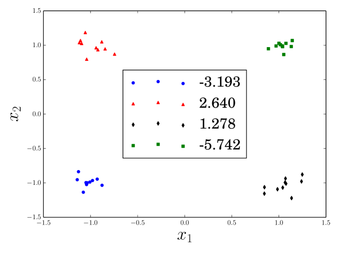
Figure 2: Hypercube-2 dataset: see main text for details.

We fix $m=1,\alpha_{s}=0.95$ and set remaining BART hyperparameters to the default values. Since the true tree has $2^{D}$ leaves, we set $\beta_{s}$ such that the expected number of leaves is roughly $2^{D}$. We run 2000 iterations of MCMC. Figure 3 illustrates the posterior trace plots for $D=4$. (See supplemental material for additional posterior trace plots.) We observe that PG converges much faster to the posterior in terms of number of leaves as well as the test MSE. We observe that GrowPrune sampler tends to overestimate the number of leaves; the low value of train MSE indicates that the GrowPrune sampler is stuck close to a mode and is unable to explore the true posterior. Pratola (2013) has reported similar behavior of GrowPrune  sampler on a different dataset as well.

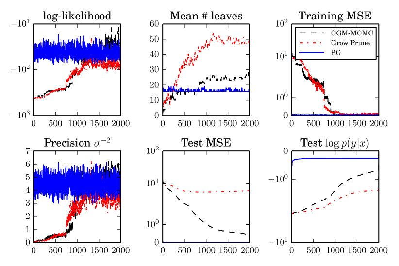
Figure 3: Results on Hypercube-4 dataset.

We compare the algorithms by computing effective sample size (ESS). ESS is a measure of how well the chain mixes and is frequently used to assess performance of MCMC algorithms; we compute ESS using R-CODA (Plummer et al., 2006). We discard the first 1000 iterations as burn-in and use the remaining 1000 iterations to compute ESS. Since the per iteration cost of generating a sample differs across samplers, we additionally report ESS per unit time. The ESS (computed using log-likelihood values) and ESS per second (ESS/s) values are shown in Tables 1 and 2 respectively. When the true tree is shallow ($D=2$ and $D=3$), we observe that CGM sampler mixes well and is computationally efficient. However, as the depth of the true tree increases ($D=4,5,7$), PG achieves much higher ESS and ESS/s compared to CGM and GrowPrune samplers.

$D$	CGM	GrowPrune	PG
2	751.66	473.57	259.11
3	762.96	285.2	666.71
4	14.01	11.76	686.79
5	2.92	1.35	667.27
7	1.16	1.78	422.96

Table 1: Comparison of ESS for CGM, GrowPrune and PG samplers on Hypercube-$D$ dataset.

$D$	CGM	GrowPrune	PG
2	157.67	114.81	7.69
3	93.01	26.94	11.025
4	0.961	0.569	5.394
5	0.130	0.071	1.673
7	0.027	0.039	0.273

Table 2: Comparison of ESS/s (ESS per second) for CGM, GrowPrune and PG samplers on Hypercube-$D$ dataset.

4.2 Real world datasets

In this experiment, we study the effect of the data dimensionality on mixing. Even when the trees are shallow, the number of trees consistent with the labels increases as the data dimensionality increases. Using the default BART prior (which promotes shallower trees), we compare the performance of the samplers on real world datasets of varying dimensionality.

We consider the CaliforniaHouses, YearPredictionMSD and CTslices datasets used by Johnson and Zhang (2013). For each dataset, there are three training sets, each of which contains 2000 data points, and a single test set. The dataset characteristics are summarized in Table 3.

Dataset	$N_{\mathsf{train}}$	$N_{\mathsf{test}}$	D
CaliforniaHouses	2000	5000	6
YearPredictionMSD	2000	51630	90
CTslices	2000	24564	384

Table 3: Characteristics of datasets.

We run each sampler using the three training datasets and report average ESS and ESS/s. All three samplers achieve very similar MSE to those reported by Johnson and Zhang (2013). The average number of leaves in the posterior trees was found to be small and very similar for all the samplers. Tables 4 and 5 respectively present results comparing ESS and ESS/s of the different samplers. As the data dimensionality increases, we observe that PG outperforms existing samplers.

$Dataset$	CGM	GrowPrune	PG
CaliforniaHouses	18.956	34.849	76.819
YearPredictionMSD	29.215	21.656	76.766
CTslices	2.511	5.025	11.838

Table 4: Comparison of ESS for CGM, GrowPrune and PG samplers on real world datasets.

$Dataset$	CGM	GrowPrune	PG
	$\times 10^{-3}$	$\times 10^{-3}$	$\times 10^{-3}$
CaliforniaHouses	1.967	48.799	16.743
YearPredictionMSD	2.018	7.029	14.070
CTslices	0.080	0.615	2.115

Table 5: Comparison of ESS/s for CGM, GrowPrune and PG samplers on real world datasets.

5 Discussion

We have presented a novel PG sampler for BART. Unlike existing samplers which make local moves, PG can propose complete trees. Experimental results confirm that PG dramatically increases mixing when the true posterior consists of deep trees or when the data dimensionality is high. While we have presented PG only for the BART model, it is applicable to extensions of BART that use a different likelihood model as well. PG can also be used along with other priors for decision trees, e.g., those of Denison et al. (1998), Wu et al. (2007) and Lakshminarayanan et al. (2014). Backward simulation (Lindsten and Schön, 2013) and ancestral sampling (Lindsten et al., 2012) have been shown to significantly improve mixing of PG for state-space models. Extending these ideas to PG-BART is a challenging and interesting future direction.

Supplementary material

Appendix A Results on hypercube$-D$ dataset

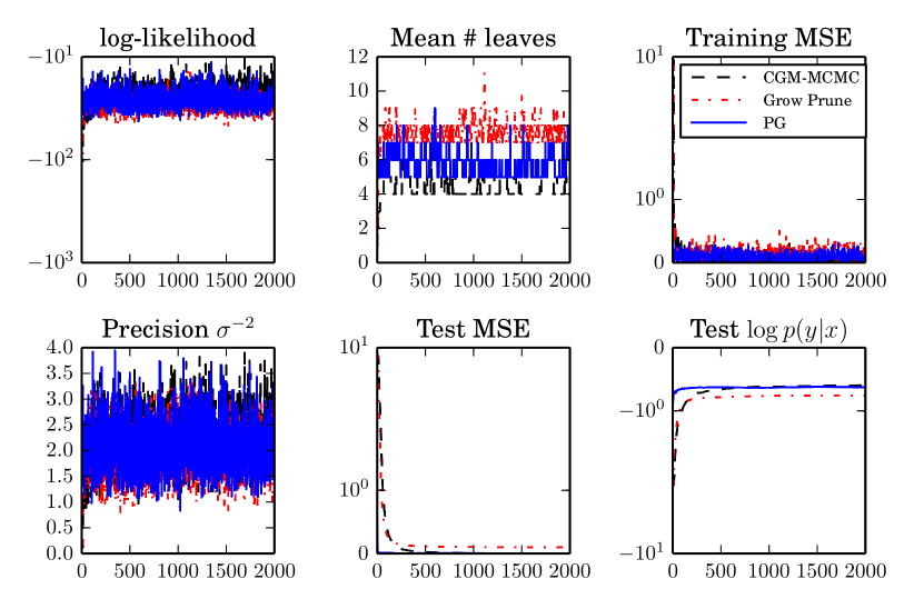
Figure 4: Results on Hypercube-2 dataset.

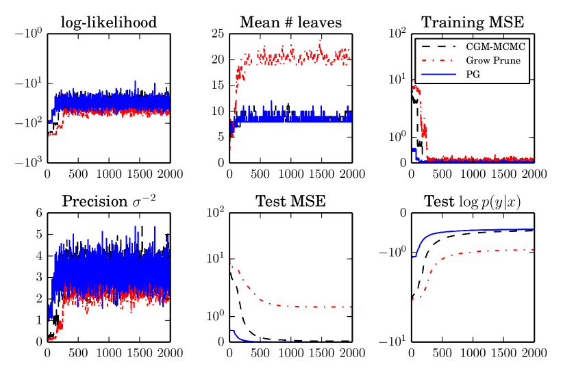
Figure 5: Results on Hypercube-3 dataset.

References

- Andrieu et al. (2010) C. Andrieu, A. Doucet, and R. Holenstein. Particle Markov chain Monte Carlo methods. J. R. Stat. Soc. Ser. B Stat. Methodol., 72(3):269–342, 2010.
- Breiman (1996) L. Breiman. Bagging predictors. Mach. Learn., 24(2):123–140, 1996.
- Breiman (2001) L. Breiman. Random forests. Mach. Learn., 45(1):5–32, 2001.
- Caruana and Niculescu-Mizil (2006) R. Caruana and A. Niculescu-Mizil. An empirical comparison of supervised learning algorithms. In Proc. Int. Conf. Mach. Learn. (ICML), 2006.
- Chipman et al. (1998) H. A. Chipman, E. I. George, and R. E. McCulloch. Bayesian CART model search. J. Am. Stat. Assoc., pages 935–948, 1998.
- Chipman et al. (2010) H. A. Chipman, E. I. George, and R. E. McCulloch. BART: Bayesian additive regression trees. Ann. Appl. Stat., 4(1):266–298, 2010.
- Denison et al. (1998) D. G. T. Denison, B. K. Mallick, and A. F. M. Smith. A Bayesian CART algorithm. Biometrika, 85(2):363–377, 1998.
- Friedman (2001) J. H. Friedman. Greedy function approximation: a gradient boosting machine. Ann. Statist, 29(5):1189–1232, 2001.
- Friedman (2002) J. H. Friedman. Stochastic gradient boosting. Computational Statistics & Data Analysis, 38(4):367–378, 2002.
- Geurts et al. (2006) P. Geurts, D. Ernst, and L. Wehenkel. Extremely randomized trees. Mach. Learn., 63(1):3–42, 2006.
- Hastie et al. (2000) T. Hastie, R. Tibshirani, et al. Bayesian backfitting (with comments and a rejoinder by the authors). Statistical Science, 15(3):196–223, 2000.
- Johnson and Zhang (2013) R. Johnson and T. Zhang. Learning nonlinear functions using regularized greedy forest. IEEE Transactions on Pattern Analysis and Machine Intelligence (TPAMI), 36(5):942-954, 2013.