Testing Chern-Simons modified gravity with orbiting superconductive gravity gradiometers
— The non-dynamical formulation

Abstract

High precision Superconductivity Gravity Gradiometers (SGG) are powerful tools for relativistic experiments. In this paper, we work out the tidal signals in non-dynamical Chern-Simons modified gravity, which could be measured by orbiting SGGs around Earth. We find that, with proper orientations of multi-axes SGGs, the tidal signals from the Chern-Simons modification can be isolated in the combined data of different axes. Furthermore, for three-axes SGGs, such combined data is the trace of the total tidal matrix, which is invariant under the rotations of SGG axes and thus free from axis pointing errors. Following nearly circular orbits, the tests of the parity-violating Chern-Simons modification and the measurements of the gravitomagnetic sector in parity-conserving metric theories can be carried out independently in the same time. A first step analysis on noise sources is also included.

1 Introduction

Among the modified gravitational theories, the extensions to the Einstein-Hilbert action with second order curvature terms are of particular interest, which may arise in the full, but still lacking, quantum theory of gravity as high energy corrections to GR, see Niedermaier2006 . The string theory inspired Chern-Simons (CS) modified gravity Deser1982 ; Campbell1990 ; Campbell1991 ; Jackiw2003 ; Alexander2009 , with the additions of a parity-violating term $R\;^{\star}R$ and a coupling scalar field $\theta$, is one of such extensions of GR. Being a promising model, CS modified gravity has found connections with different fields such as gravitational physics, particle physics, string theory, loop quantum gravity, and cosmology, please consult Alexander2009 for detailed discussions.

CS modified gravity now contains two classes of formulations, the non-dynamical and dynamical formulations, which are in fact two distinct theories. In the non-dynamical formulation, the CS scalar $\theta$ is externally prescribed. The so called canonical choice is to set $\theta$ as a linear function of coordinate time proportional inversely to a mass scale $M_{CS}$ Jackiw2003 . While, in the more realistic but complicate dynamical formulation, the evolution of the CS scalar is then sourced by the spacetime curvature. The non-dynamical formulation serves now as a useful model that provides us insights into parity-violating theories of gravity. Up to now, the experimental tests and constraints on CS gravity are all based on observations from astrophysics and space based experiments. The first but weak bound on the canonical CS scalar $\theta$ was obtained in Smith2008 based on the results from LAGEOS I, II Ciufolini2004 ; Ciufolini2010a and Gravity Probe-B Everitt2011 missions, which had constrained the CS mass scale to $M_{CS}\gtrsim 2\times 10^{-13}eV$. The strongest bounds on the canonical scalar up to now was based on the data from double binary pulsars Yunes2009a , which had the constraint $M_{CS}\gtrsim 4.7\times 10^{-10}eV$ as been revised in Ali-Haimoud2011a . For dynamical CS gravity, the vacuum solutions outside the rotating black holes and stars were studied in the slow rotation approximation in Yunes2009b ; Ali-Haimoud2011 ; Yagi2012a , and their possible tests can be found in Chen2010 ; Yagi2013 ; Vincent2013 . Moreover, the parity-violating term $R\;^{\star}R$ also leaves distinguishable signatures in gravitational waves, which may be captured by ground based or future space borne gravitational wave antennas, please consult Sopuerta2009 ; Garfinkle2010 ; Pani2011 ; Canizares2012 for details.

In experimental relativity, Braginskii and Polnarev had obtained for relativistic gravitational theories an interesting spin-quadrupole coupling between rotating sources and orbiting quadrupole oscillators Braginskii1980 ; Polnarev1986 . Along this line, the principles of detecting Earth gravitomagnetic field with orbiting gradiometers are studied in a series of works of Paik, Mashhoon and their collaborators Mashhoon1982 ; Theiss1985 ; Paik1988 ; Paik1989 ; Mashhoon1989 ; Paik2008 . Today, gradiometers have already been employed in space based experiment such as the one on GOCE satellite Rummel2011 . The high precision Superconductive Gravity Gradiometer (SGG) have been developed at the University of Maryland by Moody, Paik and their colleagues, and their performance level has already reached $2\times 10^{-11}s^{-2}/Hz^{\frac{1}{2}}$ in 1990s Moody2002 . Recently, with the improvement in cryogenics and the magnetically levitated test masses, a new design scheme with $3$ orders of magnitude improvement in the SGG performance over the frequency band $0.5mHz\sim 0.1Hz$ has been developed by this group Moody2010 ; Shirron2010 . It is also pointed out in Paik2006 that a performance level of $10^{-15}s^{-2}/Hz^{\frac{1}{2}}$ over this band is within the capability of the SGGs under development. One can consult Paik1989 ; Paik2008 ; Li2014 for the detailed error analysis of the relativistic gradient measurements with SGGs in space. On the other hand, as pointed out by Alexander, Yunes and etc. Alexander2007 ; Alexander2007a that, within the weak field and slow motion limits, the non-dynamical CS gravity differs from General Relativity (GR) only in the gravitomagnetic sector. Based on these results, we study in this work the theoretical principles of testing the parity-violating non-dynamical CS gravity with SGGs in space.

2 Signatures of gradient measurements in the non-dynamical Chern-Simons gravity

This work is heavily based on the mission concepts studied in Paik1988 ; Paik1989 ; Mashhoon1989 , that the gradient force from Earth gravitomagnetic field are measured by orbiting SGGs along nearly circular orbits. We worked out in this section the signatures of the gradient observable in non-dynamical CS gravity.

2.1 The Non-dynamical Chern-Simons modified gravity

We first give a brief introduction to the non-dynamical formulation of CS modified gravity, for detailed discussions please consult Alexander2009 ; Alexander2007 ; Alexander2007a . The geometric units $c=G=1$ are adopted in the followings. The action for non-dynamical CS gravity reads

$$S:=S_{GR}+S_{CS}+S_{matt},$$

where

$$S_{GR} = \frac{1}{16\pi}\int d^{4}x\sqrt{-g}R,\quad\>S_{CS}=\frac{\alpha}{4}\int d^{4}x\sqrt{-g}\theta R^{\star}R,$$ (1)

and $S_{matt}$ is the action from the matter fields that is independent of $\theta$. $g$ is the determinant of the metric and the Pontryagin density

$$R\;^{\star}R=\frac{1}{2}\epsilon^{cdef}R_{\;bef}^{a}R_{\;acd}^{b}.$$ (2)

The CS coupling field $\theta$ is externally prescribed and depends on the specific theory that under consideration. $\theta$ can be viewed as the deformation function, and the difference between CS gravity and GR is proportional to the deformation parameters $\nabla_{a}\theta$ and $\nabla_{a}\nabla_{b}\theta$. In the so called canonical CS coupling $\theta$ is a spatially isotropic function and depends linearly on the coordinate time $t$ Jackiw2003 , therefore the deformation parameter contains only $\dot{\theta}$.

The field equation of the non-dynamical CS gravity is obtained by varying the action with respect to the metric

$$R_{ab}-\frac{1}{2}g_{ab}R+16\pi\alpha C_{ab}=8\pi T_{ab},$$ (3)

where $C_{ab}$ is the 4-dimensional generalization of the Cotton-York tensor

$$C^{ab}=\nabla_{c}\theta\epsilon^{cde(a}\nabla_{e}R_{\;d}^{b)}+\frac{1}{2}\nabla_{c}\nabla_{d}\theta\epsilon^{efd(a}R_{\;\;\;fe}^{b)c}.$$ (4)

The introduction of the new scalar degree of freedom $\theta$ also gives rise to the new constraint

$$\nabla_{a}C^{ab}=-\frac{1}{8}\nabla^{b}\theta(^{\star}RR)=0.$$ (5)

If the above constraint is satisfied, from Eq.(3) the Bianchi identities and the equations of motion for matter fields $\nabla_{a}T^{ab}=0$ are recovered, which rank the non-dynamical CS gravity a metric theory.

In the weak field and slow motion limits, the Parametrized Post-Newtonian (PPN) metric of the non-dynamical CS gravity outside a compact source was carefully worked out in Alexander2007 ; Alexander2007a . As mentioned before, the non-dynamical CS gravity differs from GR only in the gravitomagnetic sector

$$g_{0i}^{CS}=g_{0i}^{GR}+\chi(r\nabla\times\mathbf{V})_{i},$$ (6)

here $r$ denotes the distance to the mass center of the compact source and $V_{i}$ is the PN potential, see Appendix.A. The dimensionless parameter $\chi=\frac{32\pi\alpha\dot{\theta}}{r}$ is the new PN parameter for non-dynamical CS gravity, and the CS mass scale is defined as Alexander2007 ; Alexander2007a

$$Mcs\equiv\frac{1}{8\pi\alpha\dot{\theta}}=\frac{4}{\chi r}.$$ (7)

2.2 The basic settings

We restrict ourselves to the so-called “semi-conservative” metric theories, which are based on action principles and respect the conservation law of 4-momentum Will2014 . Therefore, we work with the metric theories with four relevant standard PPN parameters $\{\gamma,\ \beta,\ \xi,\ \alpha_{1},\ \alpha_{2}\}$ together with the additional CS parameter $\chi$, please see Will2014 or Appendix.A for the PPN formalism. The PN coordinates system $\{t,x^{i}\}$ outside Earth is chosen as follows. The mass center of Earth is set at the origin. The basis $(\frac{\partial}{\partial x^{3}})^{a}$ is set to parallel to the direction of the Earth angular momentum $\mathbf{J}$, $(\frac{\partial}{\partial x^{1}})^{a}$ is pointing to a reference star $\Upsilon$ and $(\frac{\partial}{\partial x^{2}})^{a}$ determined by the right-hand rule $(\frac{\partial}{\partial x^{1}})^{a}\times(\frac{\partial}{\partial x^{2}})^{a}=(\frac{\partial}{\partial x^{3}})^{a}$. Such coordinate directions are tied to the remote stars, and the time $t$ is measured by the observers at asymptotically flat region. Within our coordinate system the PN metric outside Earth reads

$$g_{00} = -1+2U-2\beta U^{2}-2\xi\Phi_{W}+(2\gamma+2-2\xi)\Phi_{1}$$

$$+2(3\gamma-2\beta+1+\xi)\Phi_{2}+2\Phi_{3}+2(3\gamma-2\xi)\Phi_{4}$$

$$+2\xi\mathcal{A}-(\alpha_{1}-\alpha_{2})w^{2}U-\alpha_{2}w^{i}w^{j}U_{ij}-2\alpha_{1}w^{i}V_{i}+\mathcal{O}(\epsilon^{6}),$$

$$g_{0i} = -\frac{1}{2}(4\gamma+3+\alpha_{1}-\alpha_{2}-2\xi)V_{i}-\frac{1}{2}(1+\alpha_{2}+2\xi)W_{i}$$

$$+\chi r(\nabla\times\mathbf{V})^{i}-\frac{1}{2}(\alpha_{1}-2\alpha_{2})w^{i}U-\alpha_{2}w^{j}U_{ij}+\mathcal{O}(\epsilon^{5}),$$

$$g_{ij} = (1+2\gamma U)\delta_{ij}+\mathcal{O}(\epsilon^{4}),$$

please see Appendix.A for the PN potentials. For low and medium Earth orbits experiments, the magnitude of $\epsilon$ is about $10^{-5}.$

We model Earth as an ideal and uniform rotating spherical body, and for the effects from Earth gravity multiples on the gravitomeganetic field measurements with orbiting SGGs, please consult Li2014 . The preferred-frame and the preferred-location effects are tightly constrained by observations, and we now have the upper bounds of the related PN parameters as $\alpha_{1}\sim 4\times 10^{-5},\ \alpha_{2}\sim 2\times 10^{-9},\ \alpha_{3}\sim 4\times 10^{-20}$ and $\xi\sim 10^{-9}$, please see Tab.1 or Will2014 for more details. Generally, the coordinate velocity $w$ of the PPN coordinate system relative to the mean rest-frame of the universe is generally believed to be small, that $w\sim\mathcal{O}(\epsilon)$ Will1972 ; Will1993 ; Will2014 . Therefore, the gradients produced by the preferred-frame and the preferred-location effects in orbiting SGGs will be smaller than $10^{-21}s^{-2},$ which is too small to be seen by the present day SGGs and will be ignored in this work. The above metric can then be cast into a rather simple form

$$g_{\mu\nu}=$$

$$\left(\begin{array}[]{cccc}-1+\frac{2M}{r}-\frac{2\beta M^{2}}{r^{2}}&(\frac{\Delta x^{2}}{r^{3}}+\frac{3\chi x^{1}x^{3}}{2r^{4}})J&(-\frac{\Delta x^{1}}{r^{3}}+\frac{3\chi x^{2}x^{3}}{2r^{4}})J&-\frac{\chi[(x^{1})^{2}+(x^{2})^{2}-2(x^{3})^{2}]}{2r^{4}}J\\ \\ (\frac{\Delta x^{2}}{r^{3}}+\frac{3\chi x^{1}x^{3}}{2r^{4}})J&1+\frac{2\gamma M}{r}&0&0\\ \\ (-\frac{\Delta x^{1}}{r^{3}}+\frac{3\chi x^{2}x^{3}}{2r^{4}})J&0&1+\frac{2\gamma M}{r}&0\\ \\ -\frac{\chi[(x^{1})^{2}+(x^{2})^{2}-2(x^{3})^{2}]}{2r^{4}}J&0&0&1+\frac{2\gamma M}{r}\end{array}\right),$$ (15)

(16)

where $r=\sqrt{\delta_{ij}x^{i}x^{j}}$, $\Delta=1+\gamma+\frac{1}{4}\alpha_{1}$, and $M,\ \mathbf{J}$ are the asymptotically measured total mass and angular momentum of Earth

$$M = \int\rho[1+(\gamma+1)v^{2}+(3\gamma-2\beta+1)U+\frac{\Pi}{\rho}+3\gamma\frac{p}{\rho}]d^{3}x,$$

$$\mathbf{J} = \int\rho(\mathbf{x}\times\mathbf{v})d^{3}x.$$

For a satellite orbiting Earth with velocity $v,$ one has the basic order relations

$$v^{2}\sim\frac{M}{r}\sim\mathcal{O}(\epsilon^{2}),\quad\>v^{4}\sim\frac{M^{2}}{r^{2}}\sim\frac{Jv}{r^{2}}\sim\mathcal{O}(\epsilon^{4}).$$ (17)

2.3 Gravity gradient signals in non-dynamical Chern-Simons Gravity

For clearness, we set the spacecraft (S/C) that carrying the multi-axes SGG to follow a circular orbit

$$x^{1}=a\cos\Psi,\ x^{2}=a\cos i\sin\Psi,\ x^{3}=a\sin i\sin\Psi,$$ (18)

where the longitude of ascending node $\Omega$, the eccentricity $e$ are set to be zero, $i$ and $a$ denote the inclination and semi-major axis, see figure.1. $\Psi=\omega\tau$ is the orbital phase, and $\tau$ is the proper time measured by the on-board clock.

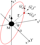
Figure 1: The orbits under consideration are circular orbits with the longitude of ascending node $\Omega=0$. As illustrated in the figure, the local tetrad carried by the S/C is defined as follows, $(\tilde{\mathbf{e}}_{1})^{a}$ is set along the direction of motion of the S/C, $(\tilde{\mathbf{e}}_{2})^{a}$ along the radial direction $\hat{\mathbf{r}}$ and $(\tilde{\mathbf{e}}_{3})^{a}=(\tilde{\mathbf{e}}_{1})^{a}\times(\tilde{\mathbf{e}}_{2})^{a}$.

We calculate the gravitational gradients measured along the above orbit for the Earth pointing option of S/C attitude. The local Earth pointing frame attached to the S/C is determined by the following local tetrad, that we set $(\tilde{\mathbf{e}}_{1})^{a}$ along the direction of motion of the S/C, $(\tilde{\mathbf{e}}_{2})^{a}$ along the radial direction $\hat{\mathbf{r}}$, $(\tilde{\mathbf{e}}_{3})^{a}=(\tilde{\mathbf{e}}_{1})^{a}\times(\tilde{\mathbf{e}}_{2})^{a}$ and $(\tilde{\mathbf{e}}_{0})^{a}=Z^{a}$ the 4-velocity of the S/C, see again figure.1. Here we do not employ the initial guided option of the S/C attitude since the gradient signal from the gravitomagnetic sector will then have twice the orbital frequency Mashhoon1989 and can hardly be separated from the far more larger signal produced by Earth $J_{2}$ component at the same frequency band. Also, as one will see, with the help of Earth pointing attitude option, the gradient signal of the CS gravity can be separated from that of the semi-conservative metric theory.

The geodesic deviation equation reads

$$Z^{b}\nabla_{b}Z^{c}\nabla_{c}\xi^{a}+R_{bcd}^{\ \ \ \ a}Z^{b}Z^{d}\xi^{c}=0,$$ (19)

where $\xi^{a}$ is the connection vector determined by the axis of the SGG. The gravitational gradient tensor or the tidal tensor is then defined as

$$\tilde{K}_{\nu}^{\ \mu}=R_{\rho\beta\lambda}^{\ \ \ \ \alpha}Z^{\rho}Z^{\lambda}\mathbf{\mathbf{e}_{\nu}^{\ \beta}\mathbf{\underline{e}_{\alpha}^{\ \mu}}},$$ (20)

here we use $\tilde{}$ to mark tensor components under the local tetrad $(\tilde{e}_{\mu})^{a}$ to distinguish the components under the original PN basis $(\frac{\partial}{\partial x^{\mu}})^{a}$, and $\mathbf{e}_{\mu}^{\ \alpha}$ denotes the transformation matrix from local frame to the Earth centered PN system, and $\mathbf{\underline{e}_{\alpha}^{\ \mu}}$ denotes the inverse. From dimensional analysis, we have

$$\tilde{K}_{\nu}^{\ \mu}=\frac{1}{a^{2}}[\underbrace{\mathcal{O}(\frac{M}{a})+\mathcal{O}(v^{2})}_{Newtonian\ terms}+\underbrace{\mathcal{O}(\frac{M^{2}}{a^{2}})+\mathcal{O}(\frac{Mv^{2}}{a})+\mathcal{O}(\frac{Jv}{a^{2}})}_{Post-Newtonian\ terms}...],$$

which means that to calculate the 1PN tidal components, that the $\frac{1}{a^{2}}\mathcal{O}(\epsilon^{4})$ terms, only the Keplerian orbits of the S/C with fixed orbital elements are needed. To evaluate the Newtonian tidal components, the 1PN correction to Keplerian orbits is then needed. However, since the Newtonian components depends only on the semi-major $a$ and the unit position vector $\hat{\mathbf{r}}$, one can then write $\hat{\mathbf{r}}$ in terms of the instantaneous orbit elements evaluated at the time of observation to work out the Newtonian tidal components. The full solutions of the 1PN orbits in CS modified gravity will be the subjects of a separated publication.

The 4-velocity of the S/C reads

$$Z^{a}=\frac{dt}{d\tau}(\frac{\partial}{\partial t})^{a}+a\omega[-\sin\Psi(\frac{\partial}{\partial x^{1}})^{a}+\cos i\cos\Psi(\frac{\partial}{\partial x^{2}})^{a}+\sin i\cos\Psi(\frac{\partial}{\partial x^{3}})^{a}].$$ (21)

The ratio $\frac{dt}{d\tau}$ can be derived from the line element $d\tau^{2}=-g_{\mu\nu}dx^{\mu}dx^{\nu}$ along the circular orbit, to the required order we have

$$\frac{dt}{d\tau} = 1+\frac{r^{2}\omega^{2}}{2}+\frac{M}{a}+\mathcal{O}(\epsilon^{4}).$$ (22)

For the tetrad attached to the reference mass defined in the last subsection, we first set $(\tilde{\mathbf{e}}_{0})^{a}=Z^{a}$, and following the Gram-Schmidt process the three spacial tetrad can be worked out to the required order as

$$(\tilde{\mathbf{e}}_{1})^{a} = a\omega(\frac{\partial}{\partial t})^{a}+(1+\frac{a^{2}\omega^{2}}{2}-\frac{\gamma M}{a})[-\sin\Psi(\frac{\partial}{\partial x^{1}})^{a}+\cos i\cos\Psi(\frac{\partial}{\partial x^{2}})^{a}$$ (23)

$$+\sin i\cos\Psi(\frac{\partial}{\partial x^{3}})^{a}],$$

$$(\tilde{\mathbf{e}}_{2})^{a} = \left(1-\frac{\gamma M}{a}\right)[\cos\Psi(\frac{\partial}{\partial x^{1}})^{a}+\cos i\sin\Psi(\frac{\partial}{\partial x^{2}})^{a}+\sin i\sin\Psi(\frac{\partial}{\partial x^{3}})^{a}],$$

$$(\tilde{\mathbf{e}}_{3})^{a} = \left(1-\frac{\gamma M}{a}\right)[\cos i(\frac{\partial}{\partial x^{3}})^{a}-\sin i(\frac{\partial}{\partial x^{2}})^{a}].$$ (25)

The transformation matrices $\mathbf{e}_{\mu}^{\ \alpha}$ and $\mathbf{\underline{e}_{\alpha}^{\ \mu}}$ are worked out to 1PN level, please see Eq.(43) and Eq.(52) in Appendix.B.

With Eq.(20), Eq.(21), and Eq.(43)-(52), the explicit forms of the 3-dimensional 1PN tidal matrix in the Earth pointing local frame can be worked out. For clarity, we move the explicit expressions in Appendix.B, please see Eq.(53)-(57) for details. These tidal matrices agree with the results in Paik1988 ; Paik1989 ; Mashhoon1989 that, in measuring the off-diagonal components of $\tilde{K}_{ij}$, the gradient signals from the gravitomagnetic sector can be separated from those produced by the Newtonian and 1PN gravitoelectric sectors. Now, the most interesting result turns out to be that the gradient signature in non-dynamical CS theory can be separated from the gravitomagnetic tidal signals of the standard parity-conserving metric theories in $\tilde{K}_{12}$ and $\tilde{K}_{23}$ components, see Eq.(55) and Eq.(56).

With a proper orientation of a two-axes diagonal-component SGG, one can read out these off-diagonal components produced by the CS modification. Denote $\hat{\mathbf{p}}$ and $\hat{\mathbf{q}}$ as the orthogonal normalized 3-vectors of the two axes of the on-board SGG, and in the S/C local frame we set

$$\hat{\mathbf{p}} = \{\frac{1}{\sqrt{2}},\ \frac{1}{\sqrt{2}},\ 0\},\ \ \ \ \hat{\mathbf{q}}=\{\frac{1}{\sqrt{2}},\ -\frac{1}{\sqrt{2}},\ 0\},$$ (26)

please see Fig.2.

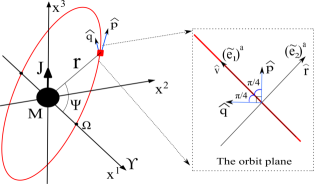
Figure 2: The configuration of the two-axes SGG along the circular orbit. The two perpendicular axes $\hat{\mathbf{p}}$ and $\hat{\mathbf{q}}$, Eq.(26), lie within the orbital plane, and they both form a angle of $\pi/4$ with the tangent vector of the orbit.

According to the tidal matrices Eq.(53)-Eq.(57), the sum and difference of the SGG read outs $\tilde{K}_{\hat{\mathbf{p}}\hat{\mathbf{p}}}$ and $\tilde{K}_{\hat{\mathbf{q}}\hat{\mathbf{q}}}$ along these two axes can be written down as

$$\tilde{K}^{+} \equiv \tilde{K}_{\hat{\mathbf{p}}\hat{\mathbf{p}}}+\tilde{K}_{\hat{\mathbf{q}}\hat{\mathbf{q}}}$$ (27)

$$= -\frac{M}{a^{3}}+\frac{(4\beta+2\gamma-3)M^{2}}{a^{4}}-\frac{(\gamma+2)\omega^{2}M}{a}$$

$$+\frac{3J\omega\Delta\cos i}{a^{3}}-2\omega_{0}^{2}-\frac{3J\chi\omega\sin i\cos\Psi}{2a^{3}},$$

$$\tilde{K}^{-} \equiv \tilde{K}_{\hat{\mathbf{p}}\hat{\mathbf{p}}}-\tilde{K}_{\hat{\mathbf{q}}\hat{\mathbf{q}}}=-\frac{J\chi\omega\sin i\sin\Psi}{2a^{3}},$$ (28)

here $\omega_{0}$ denote the angular velocity of the rotating local frame relative to the parallel transported frame. Please see Appendix.C for the explicit form of the readouts along $\hat{\mathbf{p}}$ and $\hat{\mathbf{q}}$. Therefore, for this simple two-axes SGG settings, the gradient signal produced by the CS modification can be isolated, especially in $\tilde{K}^{-}$, from those produced by the gravitomagnetic sector of the standard parity-conserving metric theory.

For the more reliable three-axes SGG options studied inPaik1988 ; Mashhoon1989 ; Paik1989 , we now set the three orthogonal SGG axes in the S/C local frame as

$$\hat{\mathbf{n}} = \{\sin\phi,\ -\cos\phi,\ 0\},$$ (29)

$$\hat{\mathbf{p}} = \frac{1}{\sqrt{2}}\{\cos\phi,\ \sin\phi,\ -1\},$$ (30)

$$\hat{\mathbf{q}} = \frac{1}{\sqrt{2}}\{\cos\phi,\ \sin\phi,\ 1\},$$ (31)

where $\phi$ is the angle between $\hat{\mathbf{n}}$ and $-\hat{\mathbf{r}}$. please see Fig.3.

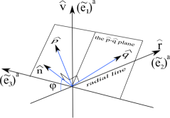
Figure 3: The configurations of three-axes SGG along the circular orbit. As in Eq.(29)-(31), The two perpendicular axes $\hat{\mathbf{p}}$ and $\hat{\mathbf{q}}$ are symmetric to the $\hat{\mathbf{r}}-\hat{\mathbf{v}}$ plane, and $\hat{\mathbf{n}}$ is orthogonal to the $\hat{\mathbf{p}}-\hat{\mathbf{q}}$ plane. The angle between $\hat{\mathbf{n}}$ and $-\hat{\mathbf{r}}$ is denoted as $\phi$.

As before, one can use the combinations of $\tilde{K}_{\hat{\mathbf{n}}\hat{\mathbf{n}}}$, $\tilde{K}_{\hat{\mathbf{p}}\hat{\mathbf{p}}}$ and $\tilde{K}_{\hat{\mathbf{q}}\hat{\mathbf{q}}}$ to single out the interested signals

$$\tilde{K}^{+} \equiv \tilde{K}_{\hat{\mathbf{p}}\hat{\mathbf{p}}}+\tilde{K}_{\hat{\mathbf{q}}\hat{\mathbf{q}}}$$ (32)

$$= \frac{M(3\cos 2\phi+1)}{2a^{3}}-\omega_{0}^{2}-\frac{((4\gamma-1)+(8\beta+8\gamma-7)\cos 2\phi)M^{2}}{4a^{4}}$$

$$+\frac{((\gamma+2)\cos 2\phi+3\gamma)M\omega^{2}}{4a}-\frac{3J\omega\Delta\cos i\cos^{2}\phi}{a^{3}}$$

$$+\frac{J\omega(\chi\sin i(3\cos 2\phi-1)\cos\Psi-2\chi\sin i\sin\phi\cos\phi\sin\Psi)}{4a^{3}},$$

$$\tilde{K}^{-} \equiv \tilde{K}_{\hat{\mathbf{p}}\hat{\mathbf{p}}}-\tilde{K}_{\hat{\mathbf{q}}\hat{\mathbf{q}}}$$ (33)

$$= \frac{3J\omega\Delta\sin i(\cos\phi\cos\Psi-3\sin\phi\sin\Psi)}{a^{3}}+\frac{J\omega\chi\cos i\cos\phi}{2a^{3}},$$

$$\tilde{K}^{\oplus} \equiv \tilde{K}_{\hat{\mathbf{p}}\hat{\mathbf{p}}}+\tilde{K}_{\hat{\mathbf{q}}\hat{\mathbf{q}}}+\tilde{K}_{\hat{\mathbf{n}}\hat{\mathbf{n}}}$$ (34)

$$= -\frac{J\chi\omega\sin i\cos\Psi}{a^{3}}+\frac{M^{2}(2\beta-\gamma-1)}{a^{4}}+\frac{(\gamma-1)M\omega^{2}}{a}-2\omega_{0}^{2}.$$

Please see Appendix.C for the explicit form of the readouts along $\hat{\mathbf{n}}$, $\hat{\mathbf{p}}$ and $\hat{\mathbf{q}}$. Therefore, without any change of the optimized three-axes configurations studied in Paik1988 ; Paik1989 ; Mashhoon1989 , the above results turns out to be quite promising. The only periodic signal in the difference $\tilde{K}^{-}$ is from the parity-conserving metric theories, which can be distinguished from the DC signal produced by the CS modification and then be used to test the gravitomagnetic sector of such theories as suggested inPaik1988 ; Paik1989 ; Mashhoon1989 ; Paik2008 . For the key result here, the only periodic signal $-\frac{J\chi\omega\sin i\cos\Psi}{a^{3}}$ in the total sums $\tilde{K}^{\oplus}$ (or the trace of the total tidal matrix) comes from the parity-violating CS modification, which can be isolated from the rest DC terms contained in $\tilde{K}^{\oplus}$.

3 The measurements of the Chern-Simons gradient signal

Recovering the SI units, the CS gradient signal to be measured is proportional to $\frac{GJ\chi\omega\sin i\cos\Psi}{c^{2}a^{3}}$. To estimate the magnitudes of the signals and the accuracy requirements for our experiment, we here assume a polar circular orbit with specific altitude as $650km$, that $a=7020km$, just like in the GP-B mission. For the three-axes SGG, the magnitude of the CS gradient signal is about $1.5\times 10^{-17}\chi s^{-2}$ with frequency about $0.17mHz$. As reported in Moody2002 , the fully developed SGG at the University of Maryland with mechanically suspended test masses has the sensitivity of $10^{-11}s^{-2}/Hz^{\frac{1}{2}}$ in the signal frequency band. For one year lifetime missions, that $t\sim\pi\times 10^{7}s$, the CS parameter $\chi$ can, in principle, be constrained to be smaller than $10^{2}$. From Eq.(7), recovering the SI units, we have

$$M_{CS}=\frac{4\hbar c}{\chi a}.$$

Therefore, for this conservative option of the SGG sensitivity, the CS mass scale can be constrained to be larger than $1.1\times 10^{-15}eV.$ This is of course a rather weak bound on the CS scalar $\theta$ or the mass scale of the theory. While, as mentioned before, the high precision SGG with performance level about $10^{-14}s^{-2}Hz^{-\frac{1}{2}}$ in the band $10^{-4}Hz\sim 10^{-1}Hz$ has already been developed at the University of Maryland Moody2010 ; Shirron2010 , and even for the performance level of $10^{-15}s^{-2}Hz^{-\frac{1}{2}}$ at the signal frequency band is within the capability of the SGGs under development Paik2006 . To be optimistic, with the likely 4 orders of magnitude improvement in the SGG performance level in the future, the CS mass scale $M_{CS}$ could be constrained to be lager than $1.1\times 10^{-11}eV$ for one year lifetime missions.

The signal to be measured will be polluted by various noises, especially those from the misalignment between axes and Earth gravity multiples. One important point is that the pointing error of the axes will not affect our measurement, since the combination $\tilde{K}^{\oplus}$ is the trace of the tidal matrix that is invariant under axes rotations. For our measurement is similar to that of the gravitomagnetic signal in the combination of $\tilde{K}^{-}$ as discussed in Paik1988 ; Mashhoon1989 ; Paik2008 , one can then consult Paik2008 ; Li2014 for the analysis of the noises from misalignments and Earth multiples. As pointed out in Paik2008 , for Earth pointing orientation, the couplings between the alignment error with Newtonian and 1PN gravitoelectric gradients will not contribute since the alignment does not modulate the these gradients in such orientation. While, for the gravitomagnetic gradient from the parity-conserving theories, its couplings with the alignment error will enter into the trace signal $\tilde{K}^{\oplus}$. But, to reach the constraint that $\chi<10^{-2}$ mentioned above one only need the misalignments to be measured to $10^{-3}rad$ in one year, which is rather an trivial task in our experiment. Thus, the test of the CS modified gravity will not suffer from the difficulties of meeting the stringent alignments and pointing requirements as in the measurements of the gravitomagnetic signal of standard parity-conserving theories. The detailed analysis concerning all these error sources will be the subjects of a future work.

At last, in the measurements of gravitomagnetic effects from parity-conserving theories, secular signals with increasing magnitude exist Mashhoon1982 ; Theiss1985 due to the frame-dragging effect that causes the SGG axes to tilt relative to Earth with angular velocity $\sim\frac{J}{a^{3}}t$ Schiff1960 ; Paik2008 . These secular signals make the detections of the gravitomagnetic effect much easier. The non-dynamical CS modified gravity differs with the parity-conserving metric theories only in the gravitomagnetic sector. Therefore, it is natural to ask whether or not similar secular gradient signals exist for the non-dynamical CS modified gravity, since the axes (or gyros) may tilt differently along the orbit due to a different gravitomagnetic torque. The answers to this problem require the studies of the 1PN geodesic motions and spin precession in the CS modified gravity, which themselves form an interesting subject and will left in our future works.

To conclude here, we studied in this paper the theoretical principles for testing non-dynamical CS modified gravity with SGGs in space. For the two-axes and three-axes diagonal-component SGGs, we worked out the characteristic signals from the CS modification in the combinations of the measurements of different axes, which can be clearly isolated in these combined data. Furthermore, for the three-axes SGG option, the precision tests of the gravitomagnetic effect in parity-conserving metric theoriesPaik1988 ; Paik1989 ; Mashhoon1989 and the test of the effects from CS modification can be carried out independently in the same time. High precision multi-axes SGGs are powerful tools for relativistic experiments, especially that carried in space, and it is promising to add the ability of testing the string theory inspired CS modified gravity to the space based experiments with orbiting SGGs.

Appendix A The standard PPN metric

The standard PPN metric has the form Will2014

$$g_{00} = -1+2U-2\beta U^{2}-2\xi\Phi_{W}+(2\gamma+2+\alpha_{3}+\zeta_{1}-2\xi)\Phi_{1}$$

$$+2(3\gamma-2\beta+1+\zeta_{2}+\xi)\Phi_{2}+2(1+\zeta_{3})\Phi_{3}+2(3\gamma+3\zeta_{4}-2\xi)\Phi_{4}$$

$$-(\zeta_{1}-2\xi)\mathcal{A}-(\alpha_{1}-\alpha_{2}-\alpha_{3})w^{2}U-\alpha_{2}w^{i}w^{j}U_{ij}+(2\alpha_{3}-\alpha_{1})w^{i}V_{i}+\mathcal{O}(\epsilon^{6}),$$

$$g_{0i} = -\frac{1}{2}(4\gamma+3+\alpha_{1}-\alpha_{2}+\zeta_{1}-2\xi)V_{i}-\frac{1}{2}(1+\alpha_{2}-\zeta_{1}+2\xi)W_{i}$$

$$-\frac{1}{2}(\alpha_{1}-2\alpha_{2})w^{i}U-\alpha_{2}w^{j}U_{ij}+\mathcal{O}(\epsilon^{5}),$$

$$g_{ij} = (1+2\gamma U)\delta_{ij}+\mathcal{O}(\epsilon^{4}),$$

where the PN potentials read

$$U = \int\frac{\rho^{\prime}}{|\mathbf{x}-\mathbf{x^{\prime}}|}d^{3}x^{\prime},\ \ \ \ \Phi_{1}=\int\frac{\rho^{\prime}v^{\prime 2}}{|\mathbf{x}-\mathbf{x^{\prime}}|}d^{3}x^{\prime},$$

$$\Phi_{2} = \int\frac{\rho^{\prime}U^{\prime}}{|\mathbf{x}-\mathbf{x^{\prime}}|}d^{3}x^{\prime},\ \ \ \ \Phi_{3}=\int\frac{\rho^{\prime}\Pi^{\prime}}{|\mathbf{x}-\mathbf{x^{\prime}}|}d^{3}x^{\prime},$$

$$\Phi_{4} = \int\frac{p^{\prime}}{|\mathbf{x}-\mathbf{x^{\prime}}|}d^{3}x^{\prime},\ \ \ \ V_{i}=\int\frac{\rho^{\prime}v^{\prime i}}{|\mathbf{x}-\mathbf{x^{\prime}}|}d^{3}x^{\prime},$$

$$W_{i} = \int\frac{\rho^{\prime}[\mathbf{v}^{\prime}\cdot(\mathbf{x}-\mathbf{x^{\prime}})](x^{i}-x^{\prime i})}{|\mathbf{x}-\mathbf{x^{\prime}}|^{3}}d^{3}x^{\prime},$$

$$U_{ij} = \int\frac{\rho^{\prime}(x^{i}-x^{\prime i})(x^{j}-x^{\prime j})}{|\mathbf{x}-\mathbf{x^{\prime}}|^{3}}d^{3}x^{\prime},$$

$$\mathcal{A} = \int\frac{\rho^{\prime}[\mathbf{v}^{\prime}\cdot(\mathbf{x}-\mathbf{x^{\prime}})]^{2}}{|\mathbf{x}-\mathbf{x^{\prime}}|^{3}}d^{3}x^{\prime},$$

$$\Phi_{W} = \int\frac{\rho^{\prime}\rho^{\prime\prime}(\mathbf{x}-\mathbf{x}^{\prime})}{|\mathbf{x}-\mathbf{x^{\prime}}|^{3}}\cdot(\frac{\mathbf{x^{\prime}}-\mathbf{x}^{\prime\prime}}{|\mathbf{x^{\prime}}-\mathbf{x}^{\prime\prime}|}-\frac{\mathbf{x}-\mathbf{x}^{\prime\prime}}{|\mathbf{x}-\mathbf{x}^{\prime\prime}|})d^{3}x^{\prime}d^{3}x^{\prime\prime}.$$

The matter variables are the rest mass density $\rho$, pressure $p$, coordinate velocity of the matter field $v^{i}$, internal energy per unit mass $\Pi$ and the coordinate velocity of the PPN coordinate system relative to the mean rest-frame of the universe $w^{i}$. The PN orders read

$$v\sim\mathcal{O}(\epsilon),\ \ \ \ v^{2}\sim U\sim\Pi\sim\frac{p}{\rho}\sim\mathcal{O}(\epsilon^{2}).$$

The standard PN parameters $\{\gamma,\ \beta,\ \xi\ ,\alpha_{1},\ \alpha_{2},\ \alpha_{3},\ \zeta_{1},\ \zeta_{2},\ \zeta_{3},\ \zeta_{4}\}$ have the following meanings. The parameters $\gamma$ and $\beta$ are the usual Eddington–Robertson–Schiff parameters used to describe the “classical” tests of GR and are in some sense the most important ones. For GR $\gamma=\beta=1$ are the only non-vanishing parameters. The parameter $\xi$ measures the preferred-location effects, $\{\alpha_{1},\ \alpha_{2},\ \alpha_{3}\}$ measure the preferred-frame effects and$\{\alpha_{3},\ \zeta_{1},\ \zeta_{2},\ \zeta_{3},\ \zeta_{4}\}$ measure the violations of global conservation laws for total momentum. The up-to-date values of these parameters are summarized in Tab.1 Will2014 .

Parameter	Bound	Experiment
$\gamma-1$	$2.3\times 10^{-5}$	time delay in Cassini tracking
	$2\times 10^{-4}$	light deflection in VLBI
$\beta-1$	$8\times 10^{-5}$	perihelion shift
	$2.3\times 10^{-4}$	Nordtvedt effect
$\xi$	$10^{-9}$	spin precession of millisecond pulsars
$\alpha_{1}$	$4\times 10^{-5}$	orbital polarization of PSR J1738+0333
	$10^{-4}$	Lunar laser ranging
$\alpha_{2}$	$2\times 10^{-9}$	spin precession of millisecond pulsars
$\alpha_{3}$	$4\times 10^{-20}$	pulsar spin down statistics
$\zeta_{1}$	0.02	combined PPN bounds
$\zeta_{2}$	$4\times 10^{-5}$	binary acceleration of PSR 1913+16
$\zeta_{3}$	$10^{-8}$	Lunar acceleration
$\zeta_{4}$	—	not independent

Table 1: Current values of PPN parameters.

Appendix B The transformation matrices and tidal matrices

From Eq.(21)-Eq.(25), the transformation matrices between the local frame and the Earth centered PN system up to 1PN level read

$$\mathbf{e=}$$

$$\left(\begin{array}[]{cccc}1+\frac{a^{2}\omega^{2}}{2}+\frac{M}{a}&-a\omega\sin\Psi&a\omega\cos i\cos\Psi&a\omega\sin i\cos\Psi\\ \\ a\omega&-(1+\frac{a^{2}\omega^{2}}{2}-\frac{\gamma M}{a})\sin\Psi&(1+\frac{a^{2}\omega^{2}}{2}-\frac{\gamma M}{a})\cos i\cos\Psi&(1+\frac{a^{2}\omega^{2}}{2}-\frac{\gamma M}{a})\sin i\sin\Psi\\ \\ 0&\left(1-\frac{\gamma M}{a}\right)\cos\Psi&\left(1-\frac{\gamma M}{a}\right)\cos i\sin\Psi&\left(1-\frac{\gamma M}{a}\right)\sin i\sin\Psi\\ \\ 0&0&-\left(1-\frac{\gamma M}{a}\right)\sin i&\left(1-\frac{\gamma M}{a}\right)\cos i\end{array}\right),$$ (42)

(43)

$$\underline{\mathbf{e}}=$$

$$\left(\begin{array}[]{cccc}1+\frac{a^{2}\omega^{2}}{2}-\frac{M}{a}&-a\omega&0&0\\ \\ a\omega\sin\Psi&-(1+\frac{a^{2}\omega^{2}}{2}+\frac{\gamma M}{a})\sin\Psi&(1+\frac{\gamma M}{a})\cos\Psi&0\\ \\ -a\omega\cos i\cos\Psi&(1+\frac{a^{2}\omega^{2}}{2}+\frac{\gamma M}{a})\cos i\cos\Psi&(1+\frac{\gamma M}{a})\cos i\sin\Psi&-(1+\frac{\gamma M}{a})\sin i\\ \\ -a\omega\sin i\cos\Psi&(1+\frac{a^{2}\omega^{2}}{2}+\frac{\gamma M}{a})\sin i\cos\Psi&(1+\frac{\gamma M}{a})\sin i\sin\Psi&(1+\frac{\gamma M}{a})\cos i\end{array}\right).$$ (51)

(52)

From Eq.(20), Eq.(21), and Eq.(43)-(52), the 3 dimensional tidal matrix $\tilde{K}_{ij}\text{$\equiv$}\tilde{K}_{ij}^{N}+\tilde{K}_{ij}^{GE}+\tilde{K}_{ij}^{GM}+\tilde{K}_{ij}^{CS}$ along the circular orbit in the Earth pointing local frame can be worked out as

$$\tilde{K}^{N}=\frac{M}{a^{3}}\left(\begin{array}[]{ccc}1&0&0\\ 0&-2&0\\ 0&0&1\end{array}\right),$$ (53)

$$\tilde{K}^{GE}=\frac{M}{a^{3}}\left(\begin{array}[]{ccc}-\frac{(2\beta+3\gamma-2)M}{a}&0&0\\ \\ 0&\frac{(6\beta+5\gamma-5)M}{a}-(\gamma+2)a^{2}\omega^{2}&0\\ \\ 0&0&\frac{(-2\beta-3\gamma+2)M}{a}+(2\gamma+1)\omega^{2}a^{2}\end{array}\right),$$ (54)

$$\tilde{K}^{GM}=\frac{J\omega}{a^{3}}\left(\begin{array}[]{ccc}0&0&-\frac{3}{2}\Delta\sin i\cos\Psi\\ \\ 0&3\Delta\cos i&\frac{9}{2}\Delta\sin i\sin\Psi\\ \\ -\frac{3}{2}\Delta\sin i\cos\Psi&\frac{9}{2}\Delta\sin i\sin\Psi&-3\Delta\cos i\end{array}\right),$$ (55)

$$\tilde{K}^{CS}=\frac{J\omega}{a^{3}}\left(\begin{array}[]{ccc}0&-\frac{1}{4}\chi\sin i\sin\Psi&-\frac{1}{4}\chi\cos i\\ \\ -\frac{1}{4}\chi\sin i\sin\Psi&-\frac{3}{2}\chi\sin i\cos\Psi&0\\ \\ -\frac{1}{4}\chi\cos i&0&\frac{1}{2}\chi\sin i\cos\Psi\end{array}\right).$$ (56)

Here, $\tilde{K}^{N}$, $\tilde{K}^{GE}$, $\tilde{K}^{GM}$ and $\tilde{K}^{CS}$ denote the gravitational tidal matrices from the Newtonian force, the 1PN gravitoelectric force, the gravitomagnetic force and the contributions from the CS modification. Since the Earth pointing frame is rotating relative to parallel transported frames (Fermi shifted), we need to include the tidal matrix from the centrifugal force produced by such rotation

$$\tilde{K}^{\omega}=-\omega_{0}^{2}\begin{pmatrix}1\\ &1\\ &&0\end{pmatrix},$$ (57)

where $\omega_{0}=\frac{d\Psi}{dt}+\frac{1}{a}\mathcal{O}(\epsilon^{3})$ denote the angular velocity of the rotation of the local frame.

Appendix C The explicit form of the gradients readouts

For the two-axes SGG discussed in Subsection.2.3, see Eq.(26) and Fig.2, the readouts along $\hat{\mathbf{p}}$ and $\hat{\mathbf{q}}$ are

$$\tilde{K}_{\hat{\mathbf{p}}\hat{\mathbf{p}}}^{\omega} = \tilde{K}_{\hat{\mathbf{q}}\hat{\mathbf{q}}}^{\omega}=-\omega_{0}^{2}\ \ \ \ \ \ \ \tilde{K}_{\hat{\mathbf{p}}\hat{\mathbf{p}}}^{N}=\tilde{K}_{\hat{\mathbf{q}}\hat{\mathbf{q}}}^{N}=-\frac{M}{2a^{3}},$$

$$\tilde{K}_{\hat{\mathbf{p}}\hat{\mathbf{p}}}^{GE} = \tilde{K}_{\hat{\mathbf{q}}\hat{\mathbf{q}}}^{GE}=\frac{(4\beta+2\gamma-3)M^{2}}{2a^{4}}-\frac{(\gamma+2)M\omega^{2}}{2a},$$

$$\tilde{K}_{\hat{\mathbf{p}}\hat{\mathbf{p}}}^{GM} = \tilde{K}_{\hat{\mathbf{q}}\hat{\mathbf{q}}}^{GM}=\frac{3\Delta J\omega\cos i}{2a^{3}},$$

$$\tilde{K}_{\hat{\mathbf{p}}\hat{\mathbf{p}}}^{CS} = -\frac{\chi J\omega\sin i(3\cos\Psi+\sin\Psi)}{4a^{3}},\ \ \ \ \ \tilde{K}_{\hat{\mathbf{q}}\hat{\mathbf{q}}}^{CS}=-\frac{\chi J\omega\sin i(3\cos\Psi-\sin\Psi)}{4a^{3}}.$$

For the three-axes SGG in Subsection.2.3, see Eq.(29)-(31) and Fig.(3), the readouts along $\hat{\mathbf{n}}$, $\hat{\mathbf{p}}$ and $\hat{\mathbf{q}}$ are

$$\tilde{K}_{\hat{\mathbf{n}}\hat{\mathbf{n}}}^{\omega} = -\omega_{0}^{2},\quad\tilde{K}_{\hat{\mathbf{p}}\hat{\mathbf{p}}}^{\omega}=\tilde{K}_{\hat{\mathbf{q}}\hat{\mathbf{q}}}^{\omega}=-\frac{\omega_{0}^{2}}{2},$$

$$\tilde{K}_{\hat{\mathbf{n}}\hat{\mathbf{n}}}^{N} = -\frac{M(3\cos 2\phi+1)}{2a^{3}},\quad\tilde{K}_{\hat{\mathbf{p}}\hat{\mathbf{p}}}^{N}=\tilde{K}_{\hat{\mathbf{q}}\hat{\mathbf{q}}}^{N}=\frac{M(3\cos 2\phi+1)}{4a^{3}},$$

$$\tilde{K}_{\hat{\mathbf{n}}\hat{\mathbf{n}}}^{GE} = \frac{\left((6\beta+5\gamma-5)\cos^{2}\phi-(2\beta+3\gamma-2)\sin^{2}\phi\right)M^{2}}{a^{4}}-\frac{(\gamma+2)\cos^{2}\phi M\omega^{2}}{a},$$

$$\tilde{K}_{\hat{\mathbf{p}}\hat{\mathbf{p}}}^{GE} = \tilde{K}_{\hat{\mathbf{q}}\hat{\mathbf{q}}}^{GE}=-\frac{((4\gamma-1)+(8\beta+8\gamma-7)\cos 2\phi)M^{2}}{4a^{4}}+\frac{((\gamma+2)\cos 2\phi+3\gamma)M\omega^{2}}{4a},$$

$$\tilde{K}_{\hat{\mathbf{n}}\hat{\mathbf{n}}}^{GM} = \frac{3\Delta J\omega\cos i\cos^{2}\phi}{a^{3}},$$

$$\tilde{K}_{\hat{\mathbf{p}}\hat{\mathbf{p}}}^{GM} = -\frac{3\Delta J\omega\left(\sin i(3\sin\phi\sin\Psi-\cos\phi\cos\Psi)+\cos i\cos^{2}\phi\right)}{2a^{3}},$$

$$\tilde{K}_{\hat{\mathbf{q}}\hat{\mathbf{q}}}^{GM} = -\frac{3\Delta J\omega\left(\sin i(-3\sin\phi\sin\Psi+\cos\phi\cos\Psi)+\cos i\cos^{2}\phi\right)}{2a^{3}},$$

$$\tilde{K}_{\hat{\mathbf{n}}\hat{\mathbf{n}}}^{CS} = \frac{J\chi\omega\sin i\cos\phi(\sin\phi\sin\Psi-3\cos\phi\cos\Psi)}{2a^{3}},$$

$$\tilde{K}_{\hat{\mathbf{p}}\hat{\mathbf{p}}}^{CS} = \frac{J\chi\omega\left(\sin i\left((1-3\sin^{2}\phi)\cos\Psi-\sin\phi\cos\phi\sin\Psi\right)+\cos i\cos\phi\right)}{4a^{3}},$$

$$\tilde{K}_{\hat{\mathbf{q}}\hat{\mathbf{q}}}^{CS} = \frac{J\chi\omega\left(\sin i\left((1-3\sin^{2}\phi)\cos\Psi-\sin\phi\cos\phi\sin\Psi\right)-\cos i\cos\phi\right)}{4a^{3}}.$$

References

• (1) M. Niedermaier, M. Reuter, Living Reviews in Relativity 9, 5 (2006). DOI 10.12942/lrr-2006-5
• (2) S. Deser, R. Jackiw, S. Templeton, Annals Phys. 140, 372 (1982)
• (3) B.A. Campbell, M.J. Duncan, N. Kaloper, K.A. Olive, Physics Letters B 251, 34 (1990). DOI 10.1016/0370-2693(90)90227-W
• (4) B.A. Campbell, M.J. Duncan, N. Kaloper, K.A. Olive, Nuclear Physics B 351, 778 (1991). DOI 10.1016/S0550-3213(05)80045-8
• (5) R. Jackiw, S.Y. Pi, Phys. Rev. D 68, 104012 (2003). DOI 10.1103/PhysRevD.68.104012. URL http://link.aps.org/doi/10.1103/PhysRevD.68.104012
• (6) S. Alexander, N. Yunes, Phys. Rept. 480, 1 (2009). DOI 10.1016/j.physrep.2009.07.002
• (7) T.L. Smith, A.L. Erickcek, R.R. Caldwell, M. Kamionkowski, Phys.Rev. D77, 024015 (2008). DOI 10.1103/PhysRevD.77.024015
• (8) I. Ciufolini, E. Pavlis, Nature 431, 958 (2004). DOI 10.1038/nature03007
• (9) I. Ciufolini, E.C. Pavlis, J. Ries, R. Koenig, G. Sindoni, A. Paolozzi, H. Newmayer, in Astrophysics and Space Science Library, Astrophysics and Space Science Library, vol. 367, ed. by I. Ciufolini, R.A.A. Matzner (2010), Astrophysics and Space Science Library, vol. 367, p. 371. DOI 10.1007/978-90-481-3735-0_17
• (10) C.W.F. Everitt, D.B. Debra, B.W. Parkinson, J.P. Turneaure, J.W. Conklin, M.I. Heifetz, G.M. Keiser, A.S. Silbergleit, T. Holmes, J. Kolodziejczak, M. Al-Meshari, J.C. Mester, B. Muhlfelder, V.G. Solomonik, K. Stahl, P.W. Worden, Jr., W. Bencze, S. Buchman, B. Clarke, A. Al-Jadaan, H. Al-Jibreen, J. Li, J.A. Lipa, J.M. Lockhart, B. Al-Suwaidan, M. Taber, S. Wang, Physical Review Letters 106(22), 221101 (2011). DOI 10.1103/PhysRevLett.106.221101
• (11) N. Yunes, D.N. Spergel, Phys. Rev. D 80, 042004 (2009). DOI 10.1103/PhysRevD.80.042004. URL http://link.aps.org/doi/10.1103/PhysRevD.80.042004
• (12) Y. Ali-Haimoud, Phys. Rev. D 83, 124050 (2011). DOI 10.1103/PhysRevD.83.124050. URL http://link.aps.org/doi/10.1103/PhysRevD.83.124050
• (13) N. Yunes, F. Pretorius, Phys. Rev. D 79, 084043 (2009). DOI 10.1103/PhysRevD.79.084043. URL http://link.aps.org/doi/10.1103/PhysRevD.79.084043
• (14) Y. Ali-Haimoud, Y. Chen, Phys. Rev. D 84, 124033 (2011). DOI 10.1103/PhysRevD.84.124033. URL http://link.aps.org/doi/10.1103/PhysRevD.84.124033
• (15) K. Yagi, N. Yunes, T. Tanaka, Phys.Rev. D86, 044037 (2012). DOI 10.1103/PhysRevD.86.044037
• (16) S. Chen, J. Jing, Class.Quant.Grav. 27, 225006 (2010). DOI 10.1088/0264-9381/27/22/225006
• (17) K. Yagi, L.C. Stein, N. Yunes, T. Tanaka, Phys. Rev. D 87, 084058 (2013). DOI 10.1103/PhysRevD.87.084058. URL http://link.aps.org/doi/10.1103/PhysRevD.87.084058
• (18) F. Vincent, Class.Quant.Grav. 31, 025010 (2013). DOI 10.1088/0264-9381/31/2/025010
• (19) C.F. Sopuerta, N. Yunes, Phys. Rev. D 80, 064006 (2009). DOI 10.1103/PhysRevD.80.064006. URL http://link.aps.org/doi/10.1103/PhysRevD.80.064006
• (20) D. Garfinkle, F. Pretorius, N. Yunes, Phys. Rev. D 82, 041501 (2010). DOI 10.1103/PhysRevD.82.041501. URL http://link.aps.org/doi/10.1103/PhysRevD.82.041501
• (21) P. Pani, V. Cardoso, L. Gualtieri, Phys. Rev. D 83, 104048 (2011). DOI 10.1103/PhysRevD.83.104048. URL http://link.aps.org/doi/10.1103/PhysRevD.83.104048
• (22) P. Canizares, J.R. Gair, C.F. Sopuerta, Phys. Rev. D 86, 044010 (2012). DOI 10.1103/PhysRevD.86.044010. URL http://link.aps.org/doi/10.1103/PhysRevD.86.044010
• (23) V.B. Braginskii, A.G. Polnarev, ZhETF Pis ma Redaktsiiu 31, 444 (1980)
• (24) A.G. Polnarev, in Relativity in Celestial Mechanics and Astrometry. High Precision Dynamical Theories and Observational Verifications, IAU Symposium, vol. 114, ed. by J. Kovalevsky, V.A. Brumberg (1986), IAU Symposium, vol. 114, pp. 401–405
• (25) B. Mashhoon, D.S. Theiss, Phys. Rev. Lett. 49, 1542 (1982). DOI 10.1103/PhysRevLett.49.1542. URL http://link.aps.org/doi/10.1103/PhysRevLett.49.1542
• (26) D.S. Theiss, Physics Letters A 109, 19 (1985). DOI 10.1016/0375-9601(85)90382-2
• (27) H.J. Paik, B. Mashhoon, C.M. Will, in Experimental Gravitational Physics, ed. by P.F. Michelson, H. En-Ke, G. Pizzella (1988), pp. 229–244
• (28) H.J. Paik, Advances in Space Research 9, 41 (1989). DOI 10.1016/0273-1177(89)90006-9
• (29) B. Mashhoon, H.J. Paik, C.M. Will, Physical Review D 39, 2825 (1989). DOI 10.1103/PhysRevD.39.2825
• (30) H.J. Paik, General Relativity and Gravitation 40, 907 (2008). DOI 10.1007/s10714-007-0582-4
• (31) R. Rummel, W. Yi, C. Stummer, Journal of Geodesy 85, 777 (2011). DOI 10.1007/s00190-011-0500-0
• (32) M.V. Moody, H.J. Paik, E.R. Canavan, Review of Scientific Instruments 73, 3957 (2002). DOI 10.1063/1.1511798
• (33) M.V. Moody, H. Paik, K.Y. Venkateswara, P.J. Shirron, M.J. Dipirro, E.R. Canavan, S. Han, P. Ditmar, R. Klees, C. Jekeli, C. Shum, AGU Fall Meeting Abstracts p. A786 (2010)
• (34) P.J. Shirron, M.J. Dipirro, E.R. Canavan, H. Paik, M.V. Moody, K.Y. Venkateswara, S. Han, P. Ditmar, R. Klees, C. Jekeli, C. Shum, AGU Fall Meeting Abstracts p. A785 (2010)
• (35) H.J. Paik, SQUID Handbook (Wiley, New York, 2006), vol. 2, pp. 545–579
• (36) X.Q. Li, M.X. Shao, H. Paik, Y.C. Huang, T.X. Song, X. Bian, General Relativity and Gravitation 46(5), 1737 (2014). DOI 10.1007/s10714-014-1737-8. URL http://dx.doi.org/10.1007/s10714-014-1737-8
• (37) S. Alexander, N. Yunes, Phys. Rev. Lett. 99, 241101 (2007). DOI 10.1103/PhysRevLett.99.241101. URL http://link.aps.org/doi/10.1103/PhysRevLett.99.241101
• (38) S. Alexander, N. Yunes, Phys. Rev. D 75, 124022 (2007). DOI 10.1103/PhysRevD.75.124022. URL http://link.aps.org/doi/10.1103/PhysRevD.75.124022
• (39) C.M. Will, Living Reviews in Relativity 17(4) (2014). DOI 10.12942/lrr-2014-4. URL http://www.livingreviews.org/lrr-2014-4
• (40) C.M. Will, J. Nordtvedt, Kenneth, Astrophys.J. 177, 757 (1972)
• (41) C. Will, Theory and experiment in gravitational physics (Cambridge University Press, 1993)
• (42) L.I. Schiff, Proceedings of the National Academy of Science 46, 871 (1960). DOI 10.1073/pnas.46.6.871