The broadening of Lyman-$\alpha$ forest absorption lines

Abstract

We provide an analytical description of the line broadening of H i absorbers in the Lyman-$\alpha$ forest resulting from Doppler broadening and Jeans smoothing. We demonstrate that our relation captures the dependence of the line-width on column density for narrow lines in $z\sim 3$ mock spectra remarkably well. Broad lines at a given column density arise when the underlying density structure is more complex, and such clustering is not captured by our model. Our understanding of the line broadening opens the way to a new method to characterise the thermal state of the intergalactic medium and to determine the sizes of the absorbing structures.

1 Introduction

The intergalactic medium (IGM) is detected as intervening absorption in the spectra of background sources (Gunn & Peterson, 1965), in the form of a ‘forest’ of H i (Lynds (1971); Weymann et al. (1981), see e.g. Rauch (1998) for a review) and He ii (Jakobsen et al., 1994; Davidsen et al., 1996) absorption lines. This gas is very highly ionised, $x=n_{\rm HI}/n_{\rm H}\sim 10^{-4}$, by a pervasive background of ionising radiation produced by galaxies and quasars (e.g. Haardt & Madau, 1996), with hints of an increasingly neutral fraction, $x\sim 0.1$, above redshift $z\sim 7$ (Mortlock et al., 2011). At all times, it contains the majority of baryons (Fukugita et al., 1998).

The growth of structure in a cold dark matter (CDM) Universe naturally gives rise to a ‘cosmic web’ of voids, sheets and filaments, with absorbers arising when the sight-line intersects higher density regions, as demonstrated in analytic models (Bi & Davidsen, 1997; Schaye, 2001) and simulations (Cen et al., 1994; Weinberg et al., 1996; Theuns et al., 1998). The temperature of this gas is set by the balance between photo-heating and adiabatic expansion and compression, resulting in a well-defined temperature-density relation, $T=T_{0}(\rho/\langle\rho\rangle)^{\gamma-1}$ , where $\gamma\approx 1$ immediately after reionisation, and $\gamma\rightarrow 1+1/1.7$ asymptotically long after reionisation (Hui & Gnedin, 1997; Theuns et al., 1998). Patchy reionisaton of either H i or He ii may lead to patchy photo-heating (Abel & Haehnelt, 1999; McQuinn et al., 2009) and hence spatial fluctuations in the temperature, but these have not (yet) been detected (Theuns et al., 2002; McQuinn et al., 2011).

Feedback from star formation is an essential ingredient in models of galaxy formation and might impact the IGM (Theuns et al., 2001). For example, elements synthesised in stars are detected in the IGM (Cowie et al., 1995), even at low densities (Schaye et al., 2003). If, as is likely, this enrichment is due to galactic winds, then the IGM might not be ideal for making cosmological inferences. Fortunately, it appears that the effects of such winds are relatively small (Theuns et al., 2002; McDonald et al., 2005; Viel et al., 2013). However, current simulations still struggle somewhat to reproduce the detected enrichment patterns as a function of density (Aguirre & Schaye, 2005; Wiersma et al., 2010; Wiersma et al., 2011) and hence may underestimate the effects of galaxy formation on the IGM.

Accurate measurements of the evolution of $T_{0}$ and $\gamma$ are interesting, since they could constrain the epoch of H i and He ii reionisation (Theuns et al., 2002), but also because the formation of small galaxies is quenched due to a reduction of atomic cooling (Efstathiou, 1992) following reionisation, and because photo-heating evaporates the gas out of shallow dark matter potentials (Okamoto et al., 2008). This is a crucial ingredient in models of galaxy formation, in particular for dwarf galaxies and satellites (Benson et al., 2002; Sawala et al., 2014). The thermal state of the IGM is also an important ‘nuisance’ factor when using the Lyman-$\alpha$ forest to study the nature of the dark matter (Boyarsky et al., 2009), or to determine the amplitude of the UV-background (Bolton et al., 2005).

Schaye et al. (1999) described a method for inferring $(T_{0},\gamma)$ from the line width versus column density ($b-N_{\rm HI}$) scatter plot of Lyman-$\alpha$ lines, when the Lyman-$\alpha$ forest is fitted as a sum of Voigt profiles for example using vpfit. This improved and extended the work of Theuns et al. (1998) who had noted that the small $b$ cut-off of the $b$-parameter distribution was sensitive to temperature. Schaye et al. (2000), and Ricotti et al. (2000); Bryan & Machacek (2000) and McDonald et al. (2001) used this to measure the $T-\rho$ relation at redshifts $z\sim 2-4$.

Since then other measurements have been performed over a larger redshift range, some also based on Voigt profile fitting (Rudie et al., 2012), or based on small-scale power spectrum or wavelet analysis (Theuns & Zaroubi, 2000; McDonald et al., 2000; Zaldarriaga et al., 2001; Theuns et al., 2002; Viel et al., 2009; Lidz et al., 2010; Garzilli et al., 2012), transmission PDF statistics (Bolton et al., 2008; Viel et al., 2009; Calura et al., 2012; Garzilli et al., 2012) and more recently on curvature statistics (Becker et al., 2011). Current measurements still have large error bars for $T_{0}$ and constraints are even poorer for $\gamma$. Bolton et al. (2008) and Viel et al. (2009) even argue that $\gamma<1$, which is difficult to understand from a theoretical point of view (McQuinn et al., 2009; Compostella et al., 2013).

The basis for all these methods is the assumption that line widths are relatively directly related to the temperature of the absorbing gas. However, it is in fact well known that - in the simulations - the absorption lines are invariably wider than just the thermal broadening. In addition there is a very large scatter in line widths at a given density, in the sense that some lines are much wider than the thermal width at a given density.

In this paper we present a new model for measuring and interpreting line widths, which builds on previous work. In our model lines are always broader that the thermal width, and we also explain the origin of the large scatter. We describe how the model can be used to infer not just $T_{0}$ and $\gamma$, but also to constrain the size of the absorbers. This paper is organised as follows. In Section 2 we begin by contrasting the ‘fluctuating Gunn-Peterson’ description of the IGM with one where the absorption is due to a distribution of individual absorbers. We do so in order to establish notation and explain the motivation for our modelling. We discuss the properties of these absorbers, and in particular what sets their line widths. In Section 3 we introduce the simulations and use them to test the basic assumptions of the model. In Section 4 we examine whether the method can in principle be applied to observables. We present a summary of our conclusions in Section 5.

2 Lyman-$\alpha$ scattering in the IGM

A Lyman-$\alpha$ photon has a large cross section for exciting a H i atom from the ground state to the electronic $n=2$ level. When the atom falls back to the ground state, the photon is in general not re-emitted in the same direction. This scattering of Lyman-$\alpha$ photons out of the sight-line to a source is usually called Lyman-$\alpha$ ‘absorption’  and is quantified by the optical depth $\tau$, such that $\exp(-\tau)$ is the resulting transmission - often referred to as the ‘flux’. We begin by calculating $\tau$ for the IGM in two very different approximations.

2.1 The fluctuating Gunn-Peterson approximation

The Lyman-$\alpha$ optical depth observed at wavelength $\lambda$ due to a homogeneous density distribution of neutral hydrogen with proper number density $n_{\rm HI}(z)$ in a cosmological setting, is given by

$$\tau(\lambda)=\int_{0}^{z_{s}}\sigma\Big{(}{\frac{(1+z)c}{\lambda}}\Big{)}\,n_{\rm HI}(z)\,\frac{c\,dz}{(1+z)H(z)}\,,$$ (1)

(Gunn & Peterson, 1965), where $c$ is the light speed, $\sigma$ is the Lyman-$\alpha$ cross section as function of frequency $c/\lambda$, $\lambda_{0}\sim 1215.67$ Å is the laboratory wavelength of the H i $n=1\rightarrow 2$ transition, and $H(z)$ the Hubble parameter at redshift $z$ (see e.g. Meiksin 2009 for an extensive recent review of the relevant physics). Since the proper length $dr$ corresponding to a redshift interval $dz$ is $dr=c\,dz/\left[(1+z)H(z)\right]$, Eq. (1) simply states that a column of neutral hydrogen $n_{\rm HI}dr$ contributes $\sigma\,n_{\rm HI}dr$ to the optical depth. Here, $z_{s}$ is the redshift of the source.

Structure formation results in the growth of the amplitude of fluctuations in the density field. This causes the transmission as a function of wavelength to be in the form of relatively well defined ‘absorbers’ (Lynds, 1971), collectively referred to as the Lyman-$\alpha$ forest (Weymann et al., 1981). At higher $z$ the absorbers blend into each other such that regions of near zero transmission are interrupted by small clearings (a Lyman-$\alpha$ jungle), whereas at low $z$ a near unity transmission is occasionally interrupted by a single absorber (a Lyman-$\alpha$ savannah).

When the gas is in photo-ionisation equilibrium, the optical depth resulting from a single absorber depends on density and temperature as $\tau\propto\rho^{2}\,T^{-0.76}$ where $T^{-0.76}$ is (approximately) the temperature dependence of the hydrogen recombination rate. Taking peculiar velocities and thermal broadening into account as well results in the ‘fluctuating Gunn-Peterson’ approximation (Gnedin & Hui, 1998; Croft et al., 1998) for the optical depth,

$$\tau(v) = \sum\int\frac{n_{\rm HI}}{1+z}\Big{|}\frac{dv^{\prime}}{dx}\Big{|}^{-1}\sigma_{\alpha}dv^{\prime}$$ (2)

$$\sigma_{\alpha} = \sigma_{0}\frac{c}{b\sqrt{\pi}}e^{-(v-v_{0})^{2}/b^{2}}$$

$$\sigma_{0} \equiv \left(\pi e^{2}\over m_{e}c\right)\left(1\over 4\pi\epsilon_{0}\right)f_{lu}\,,$$ (3)

where $e$ is the electric charge of an electron, $m_{e}$ the electron mass, $\epsilon_{0}$ is the electric constant, and $f_{lu}$ is the upward oscillator strength (usually referred to as the ‘f’ factor). The velocity coordinate $v$ is related to the observed frequency through

$$\nu = \frac{\nu_{0}}{1+\overline{z}}\left(1-\frac{v}{c}\right)\,,$$ (5)

where $\nu_{0}=c/\lambda_{0}$ is the Lyman $\alpha$ frequency in the lab, $\overline{z}$ is a mean redshift of interest. The integral is now over the profile of each individual ‘absorber’, the Jacobian $|dv^{\prime}/dx|$ takes into account velocity gradients, and the sum is over many absorbers. The Gaussian profile expresses (thermal) broadening and neglects the intrinsic line profile of the Lyman-$\alpha$ transition.

The temperature of the IGM is set by the balance between photo-ionisation heating of the UV-background, the adiabatic compression, and the adiabatic expansion of the universe. This introduces the temperature-density relation which, for densities around the cosmic mean, is approximately a power-law (Hui & Gnedin (1997))

$$T=T_{0}\,\left({\rho\over\langle\rho\rangle}\right)^{\gamma-1}\equiv T_{0}\,\Delta^{\gamma-1}\,,$$ (6)

where $T_{0}$ is the temperature at the mean density $\langle\rho\rangle$, and $\Delta$ the density contrast. Close to reionisation the gas is nearly isothermal, $\gamma\sim 1$, whereas asymptotically long after reionisation, $\gamma\rightarrow 1+1/1.7$ (Hui & Gnedin, 1997; Theuns et al., 1998). The $z<5$ Lyman-$\alpha$ forest can be reasonably well described as being a sum of of individual absorbers, and we discuss their properties next.

2.2 Lyman-$\alpha$ absorbers

The simplest single absorber, a cloud of uniform density, temperature $T$, and with HI column density $N_{\rm HI}$, produces a Gaussian absorption line when neglecting the intrinsic Lyman-$\alpha$ line profile,

$$\tau(v) = \tau_{0}e^{-(v-v_{0})^{2}/b^{2}}$$

$$\tau_{0} = \frac{\sigma_{0}c}{\sqrt{\pi}}\frac{N_{\rm HI}}{b}\,.$$ (7)

The line centre is at velocity $v_{0}=c\log(1+z)+v_{\rm pec}$ for an absorber at redshift $z$, with peculiar velocity $v_{\rm pec}$. Equation (7) can be obtained from Eq. (2) in the limit that $n_{\rm HI}|du/dx|^{-1}$ has a peak at $u_{0}$ with a width in velocity space much less than the thermal width $b$, this is the so called narrow-maximum limit in Hui et al. (1997).

Several processes contribute to the broadening $b$ of the line. The thermal broadening is given by

$$b_{T}^{2} = \frac{2k_{B}T}{m_{\rm H}}$$ (8)

$$= \left(12.8\,{\rm km~{}s}^{-1}\right)^{2}\,\,\left({\rm T_{0}\over 10^{4}~{}{\rm K}}\right)\,\Delta^{\gamma-1}\,\,,$$ (9)

with $m_{\rm H}$ the mass of the hydrogen atom and $k_{B}$ Boltzmann’s constant. The second line applies to gas on a temperature-density relation of the form $T=T_{0}\,\Delta^{\gamma-1}$ from Eq. (6).

A more realistic absorber should have at least some density structure. Assuming the line centre corresponds to a maximum $\rho_{0}$ in density, a Taylor-expansion in velocity space yields to lowest order

$$\log(\rho(v)/\rho_{0})=-(v-v_{0})^{2}/b_{\rho}^{2}\,.$$ (10)

Real Lyman-$\alpha$ absorbers may not be strongly peaked, but note that what matters is not the density profile of the absorber, but its neutral density. Since $n_{\rm HI}\propto\rho^{2}$ for isothermal gas in ionisation equilibrium, peaks in neutral gas density are better defined than the maxima in density - as we will show using numerical simulations in the next section.

The absorption profile of this more realistic absorber is then a convolution of the Gaussians of Eqs. (7) and (10), i.e. another Gaussian, with width

$$b^{2}=b_{T}^{2}+b^{2}_{\rho}\,.$$ (11)

What sets the velocity extent $b_{\rho}$? Absorbers at modest density contrast are expanding at a rate somewhat smaller than the Hubble rate, suggesting that $b_{\rho}\sim\lambda\,H$, with $\lambda$ the physical extent of the structure along the line of sight. Based on the papers of Schaye (2001) and Gnedin & Hui (1998), we expect the physical extent of the absorbers to be of the order the Jeans length $\lambda_{J}$, defined in Eq. (15) below (see also Miralda-Escude & Rees, 1993) . In the model of Schaye (2001) absorbers are assumed to be locally in near-hydrostatic equilibrium, with column density related to density by

$$N_{\rm HI}\sim n_{\rm HI}\,\lambda_{J}\,,$$ (12)

and hence ‘size’ $\lambda_{J}$. Because the dynamical times of low-density absorbers are long, the structures are still expanding, and are not exactly in hydrostatic equilibrium but are lagging behind. This is encapsulated by the ‘filtering scale’ $\lambda_{F}=2\pi/k_{F}$ of Gnedin & Hui (1998) which depends on the full history of the Jeans length over cosmic time and hence depends on the thermal history, not just the instantaneous Jeans length. The physical ‘extent’ of the absorber in this approximation is then $\sim 1/k_{F}$, therefore its velocity extent is $\sim H(z)/(k_{F}\,(1+z))\approx\lambda_{J}\,H(z)/(2\pi)$, where $\lambda_{J}$ is now the physical - as opposed to co-moving - extent of the absorber. This then motivates us to write

$$b_{\rho}=f_{J}\,{\lambda_{J}\,H(z)\over 2\pi}\,.$$ (13)

The factor $f_{J}$ parametrises the time-dependent Jeans smoothing of the gas density profiles, and we expect it to be of order unity.

For gas on a power-law temperature-density, the values of the sound speed and Jeans length depend on the density contrast $\Delta$ as

$$c_{s}^{2} = {\Big{(}\frac{5k_{\rm B}T}{3\mu m_{\rm H}}\Big{)}}$$

$$= (15.2\,{\rm km~{}s}^{-1})^{2}\,\left({T_{0}\over 10^{4}~{}{\rm K}}\right)\,\Delta^{\gamma-1}\,$$

$$\lambda_{J}^{2} \equiv {c_{s}^{2}\pi\over{\rm G}\rho_{\rm t}}$$ (15)

$$= {(5/3)\pi k_{\rm B}\,T_{0}\over\mu m_{\rm H}\,{\rm G}\rho_{t}(z=0)\,(1+z)^{3}}\,\Delta^{\gamma-2}$$

$$\approx \left(260\,{\rm kpc}\right)^{2}\,\left({T_{0}\over 10^{4}~{}{\rm K}}\right)\,\Delta^{\gamma-2}$$

$$\times \left({\Omega_{m}\over 0.307}\right)^{-1}\left({h\over 0.6777}\right)^{-2}\left({1+z\over 4}\right)^{-3}\,,$$

where $\mu$ is the mean molecular weight and $\rho_{\rm t}=\rho_{\rm dm}+\rho_{\rm b}$ is the total density, dark matter plus baryons, $G$ is the gravitational constant, $\Omega_{m}$ is the matter density. We write the Hubble parameter at redshift $z$ as $H(z)$, with $H_{0}=100h$ km s^-1 Mpc^-1 its value today. The numerical values assume $\mu=0.59$, that dark matter and gas move together, and for reference we use the Planck Collaboration et al. (2013) values for the cosmological parameters. Numerically, the broadening due to Jeans smoothing is thus of order

$$b_{\rho}^{2} = f_{J}^{2}\,{10\,k_{\rm B}T\over 9\mu\,m_{\rm H}\Delta}\,{H^{2}(z)\over H^{2}_{0}\,\Omega_{m}\,(1+z)^{3}}$$

$$\approx (11.1\,{\rm km~{}s}^{-1})^{2}\,\left({f_{J}\over 0.88}\right)^{2}\,\left({T_{0}\over 10^{4}~{}{\rm K}}\right)\,\Delta^{\gamma-2}\,\,,$$

independent of redshift in the high-redshift approximation $H(z)\propto(1+z)^{3/2}$. The model of Hui & Rutledge (1999) uses a very similar reasoning to infer line widths; $b_{\rho}$ is usually referred to as the ‘Hubble broadening’. We demonstrate below that a value of $f_{J}\sim 0.88$ describes our numerical simulations well at $z=3$.

The total broadening, $b$, of the absorber is then

$$b^{2} = b_{T}^{2}\,\left[1+f_{J}^{2}\,{5\over 9\mu}\,\Delta^{-1}\right]$$ (17)

$$\approx b_{T}^{2}\,\left[1+0.75\left({f_{J}\over 0.88}\right)^{2}\,\Delta^{-1}\right]\,.$$

The line-widths of weak absorbers ($\Delta\lower 3.22916pt\hbox{$\sim$}\hbox to0.0pt{\hss\raise 1.1625pt\hbox{$<$}}1$) are increasingly dominated by Hubble broadening, $b^{2}\sim b_{T}^{2}\,\Delta^{-1}\propto\Delta^{\gamma-2}$, and hence the filtering scales determines their widths. Hubble expansion plays a smaller role for stronger lines, with line widths ultimately set by thermal broadening alone. Equation (17) smoothly interpolates between filtering and pure thermal broadening. However, we note that for typical $z\sim 3$ absorbers with $\Delta\sim 3$, Hubble broadening still plays a significant role, increasing $b$ by almost 70 per cent compared to thermal broadening alone. It might be possible to measure the extent of absorbers in real space using close quasar pairs (see Rorai et al. (2013); the impact of Jeans length on quasar pairs was also considered in Peeples et al. (2010)). The extra broadening discussed here is a longitudinal measure of the Jeans length, as opposed to the transverse Jeans length probed with pairs.

The Gaussian shape of the absorber directly relates column density and width,

$$b^{2} = -{2\tau^{2}\over\tau\,\tau^{\prime\prime}-\tau^{\prime 2}}=-\frac{2\tau_{0}}{\tau_{0}^{\prime\prime}}\,$$ (18)

$$N_{\rm HI} = \frac{\sqrt{\pi}}{\sigma_{0}c}b\tau_{0}\,,$$ (19)

where $\tau^{\prime}\equiv d\tau/dv$, $\tau^{\prime\prime}\equiv d^{2}\tau/dv^{2}$, and the subscript 0 indicates that the quantity is to be evaluated at the (local) maximum of the optical depth. We will use these relations below. Equations (18-19) follow directly from Eqs. (7).

3 Broadening of Lyman-$\alpha$ absorbers in simulations

3.1 Mock spectra from simulations

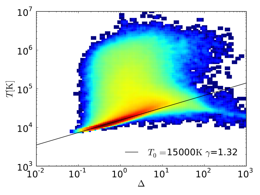
(a)

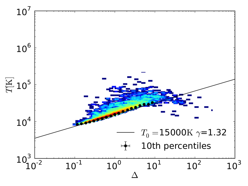
(b)

Figure 1: Mass-weighted (top panel) and optical depth weighted (bottom panel) temperature-density relation in the reference owls run at $z=3$. Values in the bottom panel are evaluated at the locations of maxima in the optical depth. Colours are a measure of the density of points in these plots, and $\Delta=\rho/\langle\rho\rangle$. In the lower panel the black dots indicate the median temperature in bins of $\Delta$ with error bars computed by bootstrap resampling. The black solid line in both panels show the power-law $T=T_{0}\Delta^{\gamma-1}$ that best fits the black dots for $\Delta<3$. There is a much larger scatter in $T$ vs $\Delta$ in the top panel than in the bottom panel, but this shocked gas contributes little to the Lyman-$\alpha$ forest. The lower-envelope of points in the $T-\Delta$ relation in the bottom panel mirrors the temperature-density relation of the lower-envelope in the top panel, demonstrating that the optical-depth weighted temperature at the optical depth maxima of absorption lines follows very closely the $T-\Delta$ relation of the photo-heated IGM.

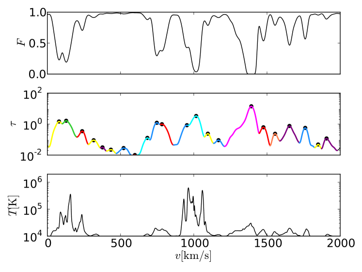
Figure 2: A stretch of a simulated spectrum at redshift $z\sim 3$. From top to bottom we show the transmission $F\equiv(-\tau)$, optical depth $\tau$, and optical depth weighted temperature, $T$, as function of velocity $v$. Individual lines are regions of the spectra between two minima in optical depth, they are coloured using different colours, with a filled circle at the maximum $\tau$ for each line. Note that $T$ is not constant over a line.

We use the reference model of the owls suite (Schaye et al., 2010) to test our model for line broadening. Briefly, the owls suite is a set of cosmological hydrodynamical simulations performed with the gadget-3 code, an improved version of gadget-2 last described by Springel (2005), with subgrid models for unresolved galaxy formation physics, in particular star formation, and feedback by and enrichment from stars, as described in Schaye & Dalla Vecchia (2008), Dalla Vecchia & Schaye (2008) and Wiersma et al. (2009), respectively. Although efficient feedback from star formation results in outflows from galaxies in this simulation, such winds do not have a significant impact on the Lyman-$\alpha$ forest for reasons discussed in Theuns et al. (2002), see also Viel et al. (2013). Most relevant for this paper is that we simulate a $\Lambda$ cold dark matter model using 512³ SPH particles that represent the gas, and an equal number of dark matter particles. The computational volume is a periodic box of co-moving size 25$h^{-1}$ Mpc on a side. The masses of the gas particles ($\sim 2\times 10^{6}h^{-1}M_{\odot}$) are sufficiently low to obtain numerical convergence for the line widths (Theuns et al., 1998). Photo-heating of the gas in the presence of an optically thin UV/X-ray background from Haardt & Madau (2001) is implemented using interpolation tables from Wiersma et al. (2009).

Photo-heating, adiabatic processes, shocks from structure formation and feedback from galactic winds and radiative cooling produce the temperature-density relation shown in Fig. 1a at redshift $z=3$. Most of the gas is on a tight temperature-density relation, $T=T_{0}\,\Delta^{\gamma-1}$, with $T_{0}\approx 15000$ K and $\gamma\approx 1.32$ for $\Delta\lower 3.22916pt\hbox{$\sim$}\hbox to0.0pt{\hss\raise 1.1625pt\hbox{$<$}}5$, and this gas is the main reservoir responsible for producing the Lyman-$\alpha$ forest. There is gas at significantly higher temperatures at these densities, which results from structure formation and feedback. The increased importance of radiative cooling decreases the amount of hot gas at higher densities, and an equilibrium sequence where radiative cooling and photo-heating balance results in the appearance of significant amounts of gas at $T\sim 10^{4}~{}$K. This higher density gas results in Lyman-limit and damped Lyman-$\alpha$ absorbers (e.g. Altay et al. 2011). Self-shielding is important for this higher-density gas, and the impact of feedback becomes more important (Altay et al., 2013).

Given a snapshot of the simulation at some redshift (we use $z=3$ in this paper), we generate mock Lyman-$\alpha$ spectra using the method described in Theuns et al. (1998) but using the interpolation tables of Wiersma et al. (2009) to relate total to neutral hydrogen density. We generate these spectra at very high resolution using pixels of width $\sim 2$ km s^-1, much narrower than any of the absorption features that appear. Importantly, we neither add noise nor instrumental broadening to mimic observed spectra - limiting our analysis to comparing our model to idealised observations. Each sight line is parallel to a coordinate axis of the simulation volume, and we use velocity pixels of size $v=H(z)L/[(1+z)N]$, where $L=25h^{-1}$ Mpc is the co-moving box size, and $N$ the number of pixels. We calculate $\tau(v)$, $T(v)$ and $\rho(v)$, where $T$ and $\rho$ are the optical depth weighted temperature and density, respectively (see Schaye et al. 1999). Unless explicitly stated, we will always use optical depth weighted quantities for variables measured from spectra.

In Fig. 1b we plot values of optical depth weighted temperature versus density, for pixels that correspond to local maxima in the optical depth from these mock spectra. Most points lie close to the lower-envelope of the points in the scatter plot, which tracks the same $T-\Delta$ relation as the lower envelope in Fig. 1a. The scatter around this relation is much less in Fig. 1b, because the shocked gas that causes the scatter to higher $T$ in Fig. 1a contributes little to the optical depth. At higher $\Delta\lower 3.22916pt\hbox{$\sim$}\hbox to0.0pt{\hss\raise 1.1625pt\hbox{$>$}}10$, $T$ decreases with increasing $\Delta$, reflecting the effects of radiative cooling also apparent in Fig. 1a.

3.2 Identifying individual absorbers

We identify individual absorbers (or ‘lines’) with regions of the spectrum between two minima in the optical depth, dissecting the whole spectrum in a set of unique stretches. An example spectrum is shown in Fig. 2, with different lines coloured differently, and with diamonds at the locations of local maxima in $\tau$. Unsurprisingly, the temperature varies across a line, and hence assigning a single temperature (or density) to a line is necessarily somewhat ambiguous. We could decide to associate to a line the maximum, the (weighted) mean or the value corresponding to the maximum of the line for any given physical quantity. In the following, where not specified otherwise, we will associate to the line the value of the physical quantity that corresponds to the optical depth weighted value evaluated at the local maximum in optical depth. This method for identifying lines is not directly applicable to observed spectra in the presence of noise. Such spectra should be smoothed to avoid incorrectly identifying noise features with small lines, however this may lead to missing true weak absorbers. Preliminary analysis shows that fitting a Gaussian over a set of contiguous pixels to calculate the derivatives that appear in Eq. (18) is promising, we will report on this in a future paper.

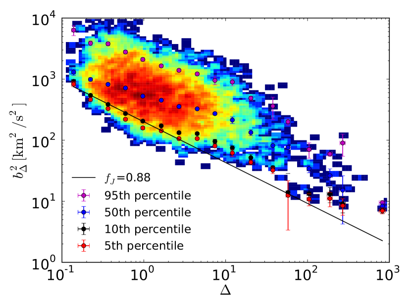
Figure 3: Velocity extent of absorbers in real space $b_{\Delta}$ versus density contrast $\Delta$ for lines identified in mock spectra without peculiar velocities. Colours indicate density of points in the plot. The 5th, 10th, 90th and 95th percentiles of $b_{\Delta}$ in bins of $\Delta$ are shown as symbols with bootstrap errors. Line widths decrease with increasing density, opposite to the case of thermal broadening. This behaviour is captured by the solid black line, the broadening $b_{\rho}$ from Eq. (13) for $f_{J}=0.88$, which fits the lower percentiles of the $b_{\Delta}-\Delta$ relation well in shape and amplitude for $\Delta\lower 3.22916pt\hbox{$\sim$}\hbox to0.0pt{\hss\raise 1.1625pt\hbox{$<$}}3$.

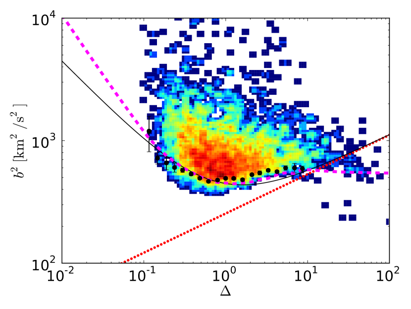
Figure 4: Total broadening $b^{2}\equiv-2\tau/\tau^{\prime\prime}$ of absorbers at line centres as a function of density contrast $\Delta$ for lines identified in mock spectra. Colours indicate density of points in the plot. Black dots with bootstrap error bars denote the location of the 10th lower percentile of $b$ in bins of $\Delta$. The dotted red line is the thermal width from Eq. 9 for the temperature-density relation from Fig. 1a; lines are invariably wider than $b_{T}$ except at $\Delta\lower 3.22916pt\hbox{$\sim$}\hbox to0.0pt{\hss\raise 1.1625pt\hbox{$>$}}10$. The solid black line is the model of Eq. (11) with $f_{J}=0.88$, for the same $T-\Delta$ power-law relation. It describes the black dots very well up to $\Delta\sim 3$, above which the simulation’s $T-\Delta$ relation is not well fit by a power-law. The dashed magenta line is again the model of Eq. (11) but now using the measured $T-\Delta$ relation rather than a power-law fit: it captures the down-turn in $b$ for $\Delta\lower 3.22916pt\hbox{$\sim$}\hbox to0.0pt{\hss\raise 1.1625pt\hbox{$>$}}3$ due to the onset of radiative cooling.

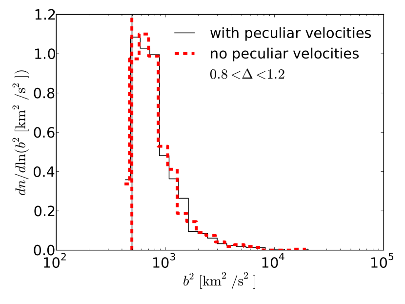
Figure 5: Histogram of line broadening $b^{2}=-2\tau/\tau^{\prime\prime}$ for simulations with and without peculiar velocities, shown as solid black and dashed red lines, respectively. The 10th percentiles of narrowest lines are indicated by vertical lines. The impact of peculiar velocities on the distribution of $b$ values is small.

As demonstrated in Fig. 1, the (real-space) temperature-density relation of the IGM in the simulation translates approximately to a power-law (optical depth weighted) temperature-density relation for the lines generated in mock spectra. Most lines follow $T=T_{0}\propto\Delta^{\gamma-1}$ up to $\Delta\lower 3.22916pt\hbox{$\sim$}\hbox to0.0pt{\hss\raise 1.1625pt\hbox{$<$}}3$, with some scatter to significantly higher $T$, but none scatter significantly below this line. However for $\Delta\lower 3.22916pt\hbox{$\sim$}\hbox to0.0pt{\hss\raise 1.1625pt\hbox{$>$}}3$, the median temperature does fall below the power law fit: this is because this gas cools radiatively, and this results in a decrease in $T$ with higher $\Delta$ for the real-space temperature-density relation as well. Note further that the $T-\Delta$ relation is only approximately a power-law, with evidence for some curvature even over a relatively narrow $\Delta$ range. Finally, note that in the absence of noise, we see that the majority of lines have $0.1\lower 3.22916pt\hbox{$\sim$}\hbox to0.0pt{\hss\raise 1.1625pt\hbox{$<$}}\Delta\lower 3.22916pt\hbox{$\sim$}\hbox to0.0pt{\hss\raise 1.1625pt\hbox{$<$}}10$.

The optical depth profile of several of the lines in Fig. 2 appear reasonably Gaussian in shape near their maxima, and we will investigate to what extent their widths follow Eq. (17). However it is also clear that some lines blend with nearby lines, and we will show below that this ‘clustering’ impacts how well we can infer the underlying $T-\Delta$ relation from spectra - even in the absence of noise.

We suggested that line broadening has a contribution $b_{\rho}$ due to the spatial extent of the absorber as described by Eq. (13). To test this directly, we should plot $b_{\rho}$ versus $\Delta$. However, maxima in $\tau$ do not correspond directly to maxima in $\Delta$ because of peculiar velocities. Therefore, to unambiguously identify a line with a density structure, we generate mock spectra setting peculiar velocities to zero. We later show that this has very little effect on the line broadening (see also Fig. 5). For each line identified in these mock spectra, we can now unambiguously identify the corresponding density stretch that gives rise to that line. However, the shape of the density structure of lines is often complex and it is not immediately apparent what extent to associate with a given line. We decided to use the following prescription. For each line we determine its start and end velocity, $v_{1}$ and $v_{2}$, the location ($v_{\rm max}$) and height ($\Delta_{\rm max}$) of the maximum density, and the integral $I\equiv\int_{v_{1}}^{v_{2}}\Delta(v)\,dv$. We now determine the value of $b_{\Delta}$ of the Gaussian profile, $G(\Delta)=\Delta_{\rm max}\,\exp(-(v-v_{\rm max})^{2}/b_{\Delta}^{2})$, for which $\int_{v_{1}}^{v_{2}}G(v)\,dv=I$. In other words, we define the extent of the absorber, $b_{\Delta}$, as the width of the Gaussian that has the same integral and maximum value as the line itself. If the line were a Gaussian, then $b_{\Delta}$ would simply be its width. Further details on the fitting procedure can be found in Appendix B. We expect that $b_{\Delta}\sim b_{\rho}$ from Eq. (13).

In Fig. 3 we plot $b^{2}_{\Delta}$ versus $\Delta$ for all lines identified in mock spectra generated while ignoring peculiar velocities. As before, colour encodes the number density of lines in this plot, and 5th, 10th, 50th and 95th percentiles are plotted as symbols with bootstrap error bars. Values of $b^{2}_{\Delta}$ increase with decreasing $\Delta$ - the opposite of what is expected from thermal broadening. The solid line indicates $b^{2}_{\rho}$ from Eq. (13) with $f_{J}=0.88$ applied to gas with the $T-\Delta$ relation $T=15000~{}{\rm K}\,\Delta^{1.3-1}$ which, as we showed earlier, fits the actual temperature-density relation of the simulation well for $0.1\lower 3.22916pt\hbox{$\sim$}\hbox to0.0pt{\hss\raise 1.1625pt\hbox{$<$}}\Delta\lower 3.22916pt\hbox{$\sim$}\hbox to0.0pt{\hss\raise 1.1625pt\hbox{$<$}}3$. Fig. 3 shows that both the 5th and 10th percentiles follow the solid line well over the same $\Delta$ range. This implies that $b_{\rho}$, with $f_{J}=0.88$, is indeed a good estimate of the width of the absorbers in real space.

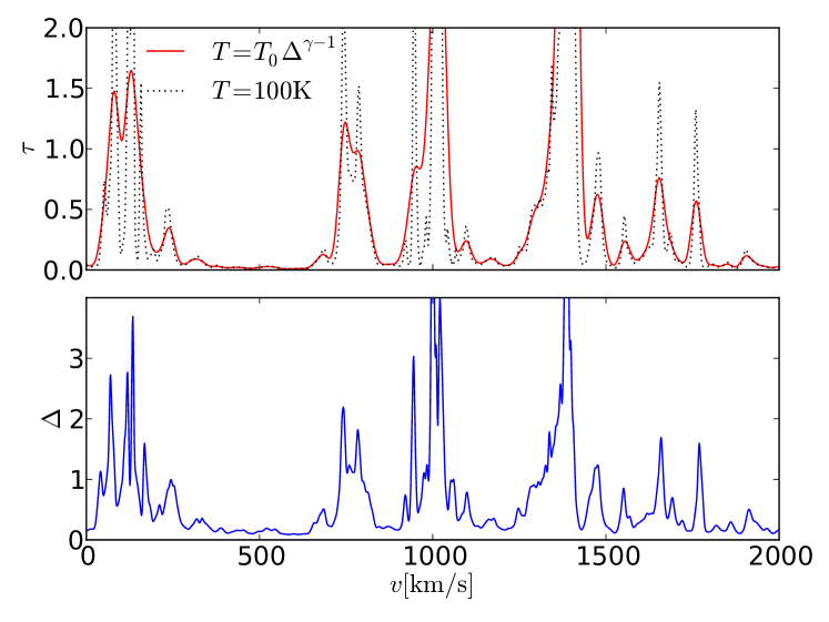
Figure 6: Optical depth $\tau$ (top panel) and corresponding density contrast $\Delta$ (bottom panel) for mock spectra for the simulation with the original temperature-density relation (solid red line) and for the case where $T=100$ K everywhere (dotted black line). Clustering of density peaks in real space makes some of the absorption lines much wider than the estimate of $b$ from Eq. (17), for example the wider lines around $v\sim 800$ km s^-1 and $v\sim 1000$ km s^-1. Thermal broadening and Hubble broadening together smooth the individual peaks seen in the underlying density field into one wide line, whose width cannot be described accurately by eq. 17.

Given that our estimate of the broadening of the density profile works well, we plot the total line broadening (including peculiar velocities) versus density contrast, and compare it to the model of Eq. (17) (Fig. 4). As before, the colour represents the density of points in the plot. We compute $b$ from the curvature of the optical depth profile $\tau(v)$ using Eq. (18); fitting a Gaussian to the pixels close to the maximum yields very similar values of $b$. Values of $b-\Delta$ for individual lines show a larger scatter in $b$ at given $\Delta$, but there is a well-defined lower envelope below which few lines appear. This lower envelope is traced by the 10th percentile of $b$ values in narrow bins of $\Delta$, plotted using black symbols with bootstrap errors. The red dashed line indicates the thermal broadening, $b_{T}$, from Eq. (9), using the power-law fit to the temperature-density relation measured in the simulation. For $\Delta\lower 3.22916pt\hbox{$\sim$}\hbox to0.0pt{\hss\raise 1.1625pt\hbox{$<$}}10$, the measured broadening along the cut-off is significantly wider than $b_{T}$, with the discrepancy between the two increasing with decreasing $\Delta$. The solid black line shows $b_{T}^{2}+b_{\rho}^{2}$ as a function of $\Delta$ from Eq. (17), again using the best-fitting power-law temperature-density relation, and adopting the value $f_{J}=0.88$ found above. It captures accurately the dependence of the broadening on $\Delta$ for the lower envelope of the absorption lines traced by the 10th percentile for $\Delta\lower 3.22916pt\hbox{$\sim$}\hbox to0.0pt{\hss\raise 1.1625pt\hbox{$<$}}3$, in particular reproducing the measured upturn in $b^{2}$ for $\Delta\lower 3.22916pt\hbox{$\sim$}\hbox to0.0pt{\hss\raise 1.1625pt\hbox{$<$}}1$. Because the solid black line assumes that the relation between temperature and density is a power law, it does not describe the simulated $b-\Delta$ relation well above $\Delta\sim 3$. The dashed black line uses the median value of the temperature at a given density for absorption lines when calculating the Jeans smoothing term $b_{\rho}$ in Eq.(13), rather than a power-law. It does much better in capturing the downturn in $b-\Delta$ at $\Delta\lower 3.22916pt\hbox{$\sim$}\hbox to0.0pt{\hss\raise 1.1625pt\hbox{$>$}}10$. We conclude from this plot that the model in which the line broadening is a combination of thermal and Jeans smoothing, Eq. (17) describes the lower-envelope in the $b-\Delta$ plane well. Note that deviations of the true temperature-density relation from a power-law, and Jeans smoothing, cause the $T-\Delta$ relation to be non-monotonic, with a minimum value of $b$ for $\Delta\sim 1$ in this particular simulation at this particular redshift.

Peculiar velocities are not the cause of the appearance of lines that are much wider than the broadening $b$ computed from Eq. (17). We compare the distribution of $b$ values for lines identified in mock spectra with and without peculiar velocities in Fig. 5. The peculiar velocities do not have a large effect on the broadening, if anything they make lines slightly narrower, see also Theuns et al. (2000).

Our analytic expression for broadening, Eq. (17), provides only a lower limit on the width of a collection of lines in the Lyman $\alpha$ forest. The additional broadening can be partially attributed to the underlying density structure in the absorber (Hui & Rutledge, 1999), for example in terms of the angle under which the sightline intersects the filament that corresponds to the absorber. However, another important contribution that is not easily captured by linear theory is the clustering of density peaks. We illustrate this in Fig. 6, comparing a mock spectrum with the original $T-\Delta$ relation with the same spectrum now computed assuming $T=100$ K everywhere. We see that some individual absorption lines identified in the solid red spectrum have several underlying density maxima. If the temperature of the gas is low, as in the case of the black dotted spectrum, then these individual density maxima give rise to their own absorption lines. But if the gas is sufficiently hot, then thermal and Hubble broadening can merge multiple individual components into one much wider line. The width of that absorber is not described well by our model. We conclude that it is the clustering of density maxima that gives rise to the lines that are much wider than expression $b$ from Eq. (17). Another way to demonstrate this is to count the number of individual density peaks for each absorber: we find that absorbers with widths close to that from Eq. (17) typically have only one density maximum, whereas those that are significantly wider correspond to several underlying peaks.

4 Inferring the temperature-density relation from observables

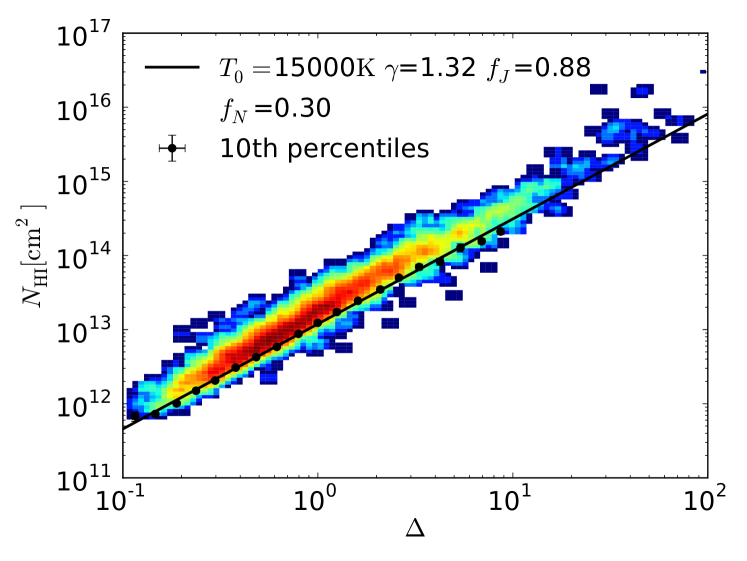
Figure 7: The neutral hydrogen column density of absorption lines versus density contrast for the reference model at $z=3$; colours are a measure of the density of points in the plot. Black dots denote the 10th percentiles of column density in logarithmic bins of $\Delta$. The solid black line corresponds to the model of Eq. (19), using the value of $\Gamma$ appropriate for the reference model with values of $T_{0}$, $\gamma$ and $f_{J}$ taken from Fig. 4, and for $f_{N}=0.3$. This value of $f_{N}$ is the result of best-fitting Eq. (19) to the 10th percentiles, for $\Delta\leq 0.3$. This provides an excellent fit to the results from the simulation over 4 orders of magnitude in column density.

Figure 8: The line-width column density $b^{2}-N_{\rm HI}$ relation in the reference owls model at redshift $z=3$, with broadening determined from Eq. (18) and column density from Eq. (19). The top axis gives the value of the density contrast that corresponds to $N_{\rm HI}$ from Eq. (23). Colours denote the density of points in this plot, black dots denote the 10th percentile of $b^{2}$ in bins of column density with bootstrap error bars. The dotted red line is the thermal broadening $b_{T}^{2}$ from Eq. (9) using Eq. (23) to relate column density to density contrast. The solid black line is our model for broadening of Eq. (25) using the values $T_{0}$ and $\gamma$ from Fig.1a, $f_{J}=0.88$ from Fig. 3 and $f_{N}=0.3$ from Fig. 7. The black line connecting magenta dashes is Eq. (25) using the $T$–$\Delta$ relation measured from the simulation, rather than a power-law fit. The analytic formula describes the minimum line width at a given column density accurately, and works even better if the actual $T-\Delta$ relation is used rather than a power-law fit.

Our description of line broadening so far used $b$ and $\Delta$ to relate temperature to density, yet density contrast $\Delta$ is not directly measurable. Here we investigate whether we can use the column density $N_{\rm HI}$ of the line instead. Following the reasoning of Schaye (2001), we make the Ansatz that the column density, density, and extent of the line are related by

$$N_{\rm HI}\sim n_{\rm HI}f_{J}\lambda_{J}\,.$$ (20)

For highly-ionised gas in photo-ionisation equilibrium

$${n_{\rm HI}\over n_{\rm H}} = \alpha_{\rm HII}n_{e}\Gamma^{-1}$$

$$\approx 5.6\times 10^{-6}\,\left({n_{\rm H}\over 1.2\cdot~{}10^{-5}~{}{\rm cm^{-3}}}\right)$$

$$\times \left({T\over 10^{4}~{}{\rm K}}\right)^{-0.76}\,\left({\Gamma\over 10^{-12}~{}{\rm s}}\right)^{-1}\,,$$

where

$$\alpha_{\rm HII} = \alpha_{0}\,\left({T\over 10^{4}{\rm K}}\right)^{-0.76}$$ (22)

$$\alpha_{0} = 4\times 10^{-13}\,{\rm cm^{3}s^{-1}}\,,$$

is the value of the case-A recombination coefficient as a function of temperature, $n_{e}$ is the electron number density, $n_{\rm H}$ is the total hydrogen number density, and $\Gamma$ the photo-ionisation rate. Combining these with the expression of the Jeans length from Eq. (15) yields

$$N_{\rm HI} = {3\sqrt{10}\over 64\pi}\,f_{N}\,f_{J}\,(2-Y)(1-Y){\Omega_{b}^{2}\over\Omega_{m}^{1/2}}{\alpha_{0}\over\Gamma}{H_{0}^{3}\over({\rm G}\,m_{\rm H})^{2}}$$ (23)

$$\times \left({k_{\rm B}\,10^{4}{\rm K}\over\mu\,m_{\rm H}}\right)^{1/2}\left({T\over 10^{4}{\rm K}}\right)^{-0.26}(1+z)^{9/2}\Delta^{3/2}$$

$$\equiv N_{0}\,\,{f_{N}\over 0.3}\,{f_{J}\over 0.88}\left({T\over 10^{4}{\rm K}}\right)^{-0.26}\Delta^{3/2}\,,$$

where numerically

$$N_{0} = 1.4\times 10^{13}\,{\rm cm}^{-2}\,\left({\Gamma\over 10^{-12}\,{\rm s}^{-1}}\right)\,\left({1+z\over 4}\right)^{9/2}$$ (24)

$$\times \left({\Omega_{b}\over 0.04825}\right)^{2}\,\left({\Omega_{m}\over 0.307}\right)^{-1/2}\,\left({h\over 0.6777}\right)^{3}\,.$$

Here, $f_{N}$ is the proportionality factor implicit in Eq. (20) which we show below is $\sim 0.3$, and the numerical value for $N_{0}$ is for very highly ionised ($\mu=0.59$) primordial gas with the Planck Collaboration et al. (2013) cosmological parameters, and $Y$ is the primordial helium abundance. For a power-law temperature-density relation, $T=T_{0}\,\Delta^{\gamma-1}$, the hydrogen column density depends only weakly on temperature, $N_{\rm HI}\propto T_{0}^{-0.26}$, and it scales with density contrast as $\Delta^{1.76-0.26\gamma}$. We compare the results from Eq. (23) to our simulation in Fig. 7, where we find the best fit of the model to the 10th percentile distribution of the $N_{\rm HI}$ versus $\Delta$, the justification of this choice is in Appendix A. The model fits very accurately the results from the simulation over nearly four order of magnitude in column density, as also shown in Rahmati et al. (2013) and Tepper-García et al. (2012).

Finally, we combine Eq. (23) with Eq. (17) to obtain a relation between the two observables quantities, namely the column density $N_{\rm HI}$ and the lower-envelope of line widths at a given column density, $b$, in terms of underlying temperature-density relation of the gas, as

$$b_{T}^{2} = {2k_{\rm B}T_{0}\over m}\,N^{(\gamma-1)/(1.76-0.26\gamma)}\,$$

$$b^{2} = b_{T}^{2}\,\left[1+0.75\,\left({f_{J}\over 0.88}\right)N^{-1/(1.76-0.26\gamma)}\right]\,$$

$$N \equiv \left({N_{\rm HI}\over N_{0}}\right)\left({T_{0}\over 10^{4}{\rm K}}\right)^{0.26}\,\left({f_{N}\over 0.3}\right)^{-1}\,\left({f_{J}\over 0.88}\right)^{-1}\,.$$ (25)

This relation is compared to the $b-N_{\rm HI}$ distribution of the simulation in Fig. 8. Our model for line broadening does well in predicting the minimum line width as a function of column density, in particular predicting correctly that line width is not a monotonic function of column density. At low $\Delta$, line widths increase as Jeans smoothing becomes more important, whereas at high $\Delta$, line widths decrease due to radiative cooling. The underlying $T-\Delta$ relation of the simulation is only approximately a power law: using the relation from the simulation directly in Eq. (23) improves the agreement between model and simulation further, in particular it might be possible to measure the temperature of denser gas, $\Delta\sim 10$. We illustrate the sensitivity of the $b-N_{\rm HI}$ relation to small changes in $T_{0}$ and $\gamma$, as well as the fitting parameters $f_{J}$ and $f_{N}$, in Appendix C.

Our model overestimates line broadening of very weak lines, $N_{\rm HI}\lower 3.22916pt\hbox{$\sim$}\hbox to0.0pt{\hss\raise 1.1625pt\hbox{$<$}}10^{12.5}$ cm^-2, yet it correctly predicts line widths at low density contrast (see Fig. 4). In Appendix A we show that this is because line width biases how well a line of given column can be associated with a given density contrast. In practise these lines are too weak to be detected in observed spectra.

5 Conclusions

We have presented an analytic description of the broadening of lines in the Lyman-$\alpha$ forest, in terms of the temperature, Jeans smoothing and density of the absorbers. Identifying individual absorbers in a spectrum as spectral stretches between two minima in the optical depth, we calculated the line width, $b$, from the second derivative of the optical depth at the local maximum in $\tau$, $b^{2}\equiv-2\tau/\tau^{\prime\prime}$ (Eq.18). We argued that the thermal width of a line, $b_{T}$, combined with its width due to Jeans smoothing, $b_{\rho}$, sets a lower-limit on the total line width, $b^{2}\lower 3.22916pt\hbox{$\sim$}\hbox to0.0pt{\hss\raise 1.1625pt\hbox{$>$}}b_{T}^{2}+b_{\rho}^{2}$. We derived an expression for $b_{\rho}$ that depends on the temperature $T$ and the density contrast $\Delta$ of the absorber, which smoothly interpolates between the filtering length interpretation of line-widths from Hui & Gnedin (1997) at low $\Delta$, and the near hydrostatic equilibrium model of Schaye (2001) at higher $\Delta$. This model gives a good description of the lower values of $b$ at given $\Delta$ (Fig. 4) . We also discussed the origin of the lines that are significantly wider than the lower envelope, arguing that they result from the clustering of several individual density maxima that cannot be distinguished in the spectrum due to thermal broadening and Jeans smoothing. Such clustering is not captured by our quasi-linear model.

Based on the model of Schaye (2001), we write an expression relating column density to density contrast. Combining this with our model for line broadening yields an analytic expression for the lower envelope of $b$ as a function of column density, $N_{\rm HI}$ (Eq. 25). This model describes the lower envelope much better than one based on thermal broadening alone (Fig. 8) .

In our interpretation of $b$, line widths of weaker lines are dominated by the filtering length, which in principle depends on the thermal history of the IGM and not just on its instantaneous state. If this is true, then not taking this into account may affect the interpretation of the $b-N_{\rm HI}$ cut-off in terms of the underlying temperature-density relation of the gas.

Our analytic description of the line broadening opens the way to a new method for determining the IGM thermal state, and in particular for measuring the ‘longitudinal’ size of the absorbers (the ‘filtering length’), that is complementary to what can be measured from close QSO pairs. This is particularly interesting, because for the first time we have a method to estimate the sizes of the clouds from a single line of sight.

6 Acknowledgement

AG thanks the Astrophysical Sector in SISSA for providing computing facilities during the realization of this paper, Carlos Frenk and Carlton Baugh for supporting her visit at ICC in Durham University, Matteo Viel for supporting her visit at Osservatorio Astronomico di Trieste, and Uroš Seljak for appointing her as a postdoctoral fellow at Ewha Womans University. This work has been partially done during her permanence at the Institute for Early Universe at Ewha Womans University, and it was supported by the WCU grant no. R32-10130 and the Research fund no. 1-2008-2935-001-2 by Ewha Womans University. AG thanks Jeroen Franse for the English revision of part of the manuscript. She also thanks Fedele Lizzi for being her mentor over many years. JS acknowledges support from the European Research Council under the European Union’s Seventh Framework Programme (FP7/2007-2013)/ERC Grant agreement 278594-GasAroundGalaxies. This work was supported by the Science and Technology Facilities Council [grant number ST/F001166/1], and by the Interuniversity Attraction Poles Programme initiated by the Belgian Science Policy Office ([AP P7/08 CHARM], and used the DiRAC Data Centric system at Durham University, operated by the Institute for Computational Cosmology on behalf of the STFC DiRAC HPC Facility (www.dirac.ac.uk). This equipment was funded by BIS National E-infrastructure capital grant ST/K00042X/1, STFC capital grant ST/H008519/1, and STFC DiRAC Operations grant ST/K003267/1 and Durham University. DiRAC is part of the National E-Infrastructure. The data used in the work is available through collaboration with the authors.

Appendix A Biases in the $N_{\rm HI}$–$\Delta$ relation

Figure 9: Density contrast - column density $\Delta$–$N_{\rm HI}$ relation for lines from the reference model, coloured according to their line width, $b$; black dots denote the 10th percentile lowest value of column-density at given density contrast. Line width $b$ and column density $N_{\rm HI}$ are calculated from Eqs. (18-19), respectively. The solid black line is the analytic relation from Eq. (23). At given $\Delta$, broader lines have higher column density, illustrating that line width biases the column density associated with a given density contrast.

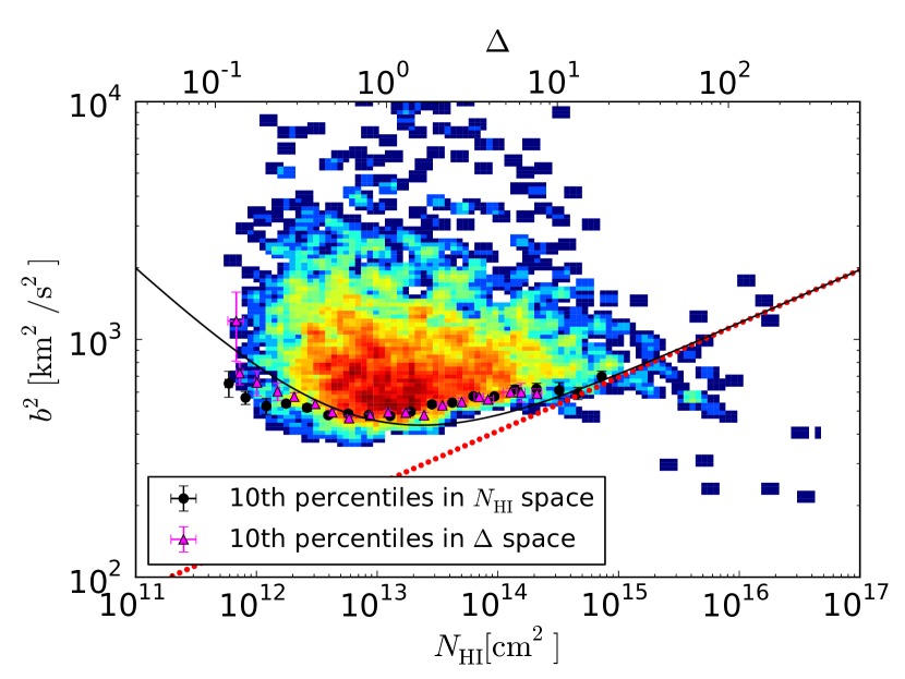
Figure 10: Column-density line width $N_{\rm HI}$-$b$ relation for the reference model, colours are a measure of the density of points in the plot; the black line is the model illustrated in Fig. 8; the dotted red line is the thermal width. Black dots denote the 10th percentile lowest values of $b$ for bins in column density, magenta triangles denote the 10th percentile lowest values of $b$ for bins in density contrast $\Delta$, using Eq. (23) to convert $\Delta$ to $N_{\rm HI}$. The bias that line width introduces in this relation causes the black dots and red dots to diverge at low $N_{\rm HI}$.

Figure 11: Same as Fig. 9, but with $N_{\rm HI}$ computed from Eq. (26). For the low-density lines the neutral hydrogen column density deviates from Eq. (23) due to the blending of the faint lines.

Figure 12: Same as Fig. 9 and 11, but with $N_{\rm HI}$ computed from Eq. (27). The distribution $\Delta$–$N_{\rm HI}$ looks similar to the one shown in Fig. 9.

In Fig. 9 we plot $\Delta$–$N_{\rm HI}$ for lines, with $N_{\rm HI}$ computed from Eq. (19), and individual lines coloured with the value of the broadening $b$, calculated from Eq. (18). Line width biases the value of column density, in the sense that the analytic model of Eq. (23) (black line in the figure) yields lower values of $N_{\rm HI}$ than Eq. (19) for broad lines. The effect of this bias on the $N_{\rm HI}$-$b$ relation is illustrated in Fig. 10. Our model for line broadening (black line) works better when lines are characterised by their density contrast (red dots) than by column density (black dots), especially for weak lines. This is because relation Eq. (23) is fitted to narrower lines.

Here we also show that Eq. (19) is equivalent to computing $N_{\rm HI}$ with the integral of the optical depth, as it is often done in the literature. In Fig. 11 we show $\Delta$–$N_{\rm HI}$, with $N_{\rm HI}$ computed from

$$N_{\rm HI} = \frac{1}{\sigma_{0}c}\int_{v_{1}}^{v_{2}}\tau\,dv\,,$$ (26)

where $v_{1}$ and $v_{2}$ are the extremes of the line. If we compare Fig. 11 with Fig. 9, we can see that Eq. (26) underestimates the neutral hydrogen column density for the low-density lines.

When lines are blended, the column density computed from Eq. (26) may become smaller and smaller as a shorter velocity interval is associated with the line (i.e. when $v_{1}\approx v_{2}$). We can estimate the contribution of these wings, and compute a corrected column-density

$$N_{\rm HI} = \frac{1}{\sigma_{0}c}\int_{-\infty}^{\infty}\tau\,dv\,,$$ (27)

by extrapolating a Gaussian fit to the line. Such an extrapolated density is closer to what is done in Voigt-profile fitting. Using Eq. (27) results in a $b-N_{\rm HI}$ distribution which is very similar from that obtained in Fig. 9, as shown in Fig. 12.

Appendix B Determination of $f_{J}$

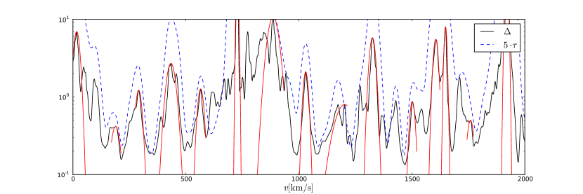
Figure 13: Density profile of absorbers in the absence of peculiar velocities (black line) for a mock spectrum calculated from the reference model; dashed blue line is the scaled optical depth for comparison. Red lines are Gaussian profiles from Eq. (10), where the width is such that the integral of the density profile of the Gaussian is the same as the one of the multi-peaked absorber. The widths of the red Gaussians are often a good approximation to the extent of an absorber.

In this Appendix we illustrate that our estimate for the extent of absorbers in real space indeed is a good approximation for their actual size. We begin by neglecting peculiar velocities (i.e. generate mock spectra after zeroing all peculiar velocities), so that we can unambiguously identify the real-space density structure that gives rise to a given line; we demonstrated in the main text that peculiar velocities have little impact on line-widths. Often individual absorption lines correspond to more than one density peak. Such clustering of peaks sometimes gives rise to very wide lines, as we argued in the text.

In Fig. 13 we show how we have computed the broadening $b_{\Delta}$ in Fig. 3 from the density profile of the multi-peaked absorber. The red lines are Gaussian profiles as in Eq. (10), with $v_{0}$ and $\rho_{0}$ respectively the velocity and the density of the local maximum in optical depth. The width $b_{\Delta}$ is such that the integral of the Gaussian density profile is the same as the integral of the density profile of the absorbers. Even though there is often no unique way of associating a ‘size’ with such complex absorbers, we believe $b_{\Delta}$ is often a good approximation of the extent over which the density contrast of an absorber is significant.

Appendix C Degeneracy of parameters in the line broadening relation

For completeness we illustrate the sensitivity of Eq. (17) to changes in the $T-\Delta$ relation (varying $T_{0}$ and $\gamma$; Fig.14), and varying the fitting parameters $f_{J}$ and $f_{N}$ (Fig. 15)

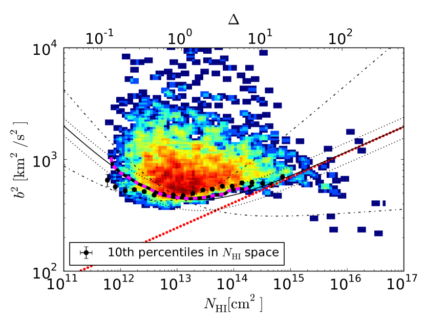
Figure 14: Same as figure 8. The dashed (dashed-dot) lines are the model from Eq. 25 with $T_{0}$ ($\gamma$) changed by $\pm 20$%.

Figure 15: Same as figure 8. The dashed (dashed-dot) lines are the model from Eq. 25 with $f_{J}$ ($f_{N}$) changed by $\pm 10$%.

References

- Abel & Haehnelt (1999) Abel T., Haehnelt M. G., 1999, ApJ, 520, L13
- Aguirre & Schaye (2005) Aguirre A., Schaye J., 2005, in Williams P., Shu C.-G., Menard B., eds, IAU Colloq. 199: Probing Galaxies through Quasar Absorption Lines Observational tests of intergalactic enrichment models. pp 289–294
- Altay et al. (2013) Altay G., Theuns T., Schaye J., Booth C. M., Dalla Vecchia C., 2013, MNRAS, 436, 2689
- Altay et al. (2011) Altay G., Theuns T., Schaye J., Crighton N. H. M., Dalla Vecchia C., 2011, ApJ, 737, L37
- Becker et al. (2011) Becker G. D., Bolton J. S., Haehnelt M. G., Sargent W. L. W., 2011, MNRAS, 410, 1096
- Benson et al. (2002) Benson A. J., Lacey C. G., Baugh C. M., Cole S., Frenk C. S., 2002, MNRAS, 333, 156
- Bi & Davidsen (1997) Bi H., Davidsen A. F., 1997, ApJ, 479, 523
- Bolton et al. (2005) Bolton J. S., Haehnelt M. G., Viel M., Springel V., 2005, MNRAS, 357, 1178
- Bolton et al. (2008) Bolton J. S., Viel M., Kim T.-S., Haehnelt M. G., Carswell R. F., 2008, MNRAS, 386, 1131
- Boyarsky et al. (2009) Boyarsky A., Lesgourgues J., Ruchayskiy O., Viel M., 2009, J. Cosmology Astropart. Phys, 5, 12
- Bryan & Machacek (2000) Bryan G. L., Machacek M. E., 2000, ApJ, 534, 57
- Calura et al. (2012) Calura F., Tescari E., D’Odorico V., Viel M., Cristiani S., Kim T.-S., Bolton J. S., 2012, MNRAS, 422, 3019
- Cen et al. (1994) Cen R., Miralda-Escudé J., Ostriker J. P., Rauch M., 1994, ApJ, 437, L9
- Compostella et al. (2013) Compostella M., Cantalupo S., Porciani C., 2013, MNRAS
- Cowie et al. (1995) Cowie L. L., Songaila A., Kim T.-S., Hu E. M., 1995, AJ, 109, 1522
- Croft et al. (1998) Croft R. A. C., Weinberg D. H., Katz N., Hernquist L., 1998, ApJ, 495, 44
- Dalla Vecchia & Schaye (2008) Dalla Vecchia C., Schaye J., 2008, MNRAS, 387, 1431
- Davidsen et al. (1996) Davidsen A. F., Kriss G. A., Zheng W., 1996, Nature, 380, 47
- Efstathiou (1992) Efstathiou G., 1992, MNRAS, 256, 43P
- Fukugita et al. (1998) Fukugita M., Hogan C. J., Peebles P. J. E., 1998, ApJ, 503, 518
- Garzilli et al. (2012) Garzilli A., Bolton J. S., Kim T.-S., Leach S., Viel M., 2012, MNRAS, 424, 1723
- Gnedin & Hui (1998) Gnedin N. Y., Hui L., 1998, MNRAS, 296, 44
- Gunn & Peterson (1965) Gunn J. E., Peterson B. A., 1965, ApJ, 142, 1633
- Haardt & Madau (1996) Haardt F., Madau P., 1996, ApJ, 461, 20
- Haardt & Madau (2001) Haardt F., Madau P., 2001, in Neumann D. M., Tran J. T. V., eds, Clusters of Galaxies and the High Redshift Universe Observed in X-rays Modelling the UV/X-ray cosmic background with CUBA
- Hui & Gnedin (1997) Hui L., Gnedin N. Y., 1997, MNRAS, 292, 27
- Hui et al. (1997) Hui L., Gnedin N. Y., Zhang Y., 1997, ApJ, 486, 599
- Hui & Rutledge (1999) Hui L., Rutledge R. E., 1999, ApJ, 517, 541
- Jakobsen et al. (1994) Jakobsen P., Boksenberg A., Deharveng J. M., Greenfield P., Jedrzejewski R., Paresce F., 1994, Nature, 370, 35
- Lidz et al. (2010) Lidz A., Faucher-Giguère C.-A., Dall’Aglio A., McQuinn M., Fechner C., Zaldarriaga M., Hernquist L., Dutta S., 2010, ApJ, 718, 199
- Lynds (1971) Lynds R., 1971, ApJ, 164, L73
- McDonald et al. (2001) McDonald P., Miralda-Escudé J., Rauch M., Sargent W. L. W., Barlow T. A., Cen R., 2001, ApJ, 562, 52
- McDonald et al. (2000) McDonald P., Miralda-Escudé J., Rauch M., Sargent W. L. W., Barlow T. A., Cen R., Ostriker J. P., 2000, ApJ, 543, 1
- McDonald et al. (2005) McDonald P., Seljak U., Cen R., Bode P., Ostriker J. P., 2005, MNRAS, 360, 1471
- McQuinn et al. (2011) McQuinn M., Hernquist L., Lidz A., Zaldarriaga M., 2011, MNRAS, 415, 977
- McQuinn et al. (2009) McQuinn M., Lidz A., Zaldarriaga M., Hernquist L., Hopkins P. F., Dutta S., Faucher-Giguère C.-A., 2009, ApJ, 694, 842
- Meiksin (2009) Meiksin A. A., 2009, Reviews of Modern Physics, 81, 1405
- Miralda-Escude & Rees (1993) Miralda-Escude J., Rees M. J., 1993, MNRAS, 260, 617
- Mortlock et al. (2011) Mortlock D. J., Warren S. J., Venemans B. P., Patel M., Hewett P. C., McMahon R. G., Simpson C., Theuns T., Gonzáles-Solares E. A., Adamson A., Dye S., Hambly N. C., Hirst P., Irwin M. J., Kuiper E., Lawrence A., Röttgering H. J. A., 2011, Nature, 474, 616
- Okamoto et al. (2008) Okamoto T., Gao L., Theuns T., 2008, MNRAS, 390, 920
- Peeples et al. (2010) Peeples M. S., Weinberg D. H., Davé R., Fardal M. A., Katz N., 2010, MNRAS, 404, 1295
- Planck Collaboration et al. (2013) Planck Collaboration Ade P. A. R., Aghanim N., Armitage-Caplan C., Arnaud M., Ashdown M., Atrio-Barandela F., Aumont J., Baccigalupi C., Banday A. J., et al. 2013, ArXiv e-prints
- Rahmati et al. (2013) Rahmati A., Pawlik A. H., Raičevic M., Schaye J., 2013, MNRAS, 430, 2427
- Rauch (1998) Rauch M., 1998, ARA&A, 36, 267
- Ricotti et al. (2000) Ricotti M., Gnedin N. Y., Shull J. M., 2000, ApJ, 534, 41
- Rorai et al. (2013) Rorai A., Hennawi J. F., White M., 2013, ApJ, 775, 81
- Rudie et al. (2012) Rudie G. C., Steidel C. C., Pettini M., 2012, ApJ, 757, L30
- Sawala et al. (2014) Sawala T., Frenk C. S., Fattahi A., Navarro J. F., Bower R. G., Crain R. A., Dalla Vecchia C., Furlong M., Jenkins A., McCarthy I. G., Qu Y., Schaller M., Schaye J., Theuns T., 2014, ArXiv e-prints
- Schaye (2001) Schaye J., 2001, ApJ, 559, 507
- Schaye et al. (2003) Schaye J., Aguirre A., Kim T.-S., Theuns T., Rauch M., Sargent W. L. W., 2003, ApJ, 596, 768
- Schaye & Dalla Vecchia (2008) Schaye J., Dalla Vecchia C., 2008, MNRAS, 383, 1210
- Schaye et al. (2010) Schaye J., Dalla Vecchia C., Booth C. M., Wiersma R. P. C., Theuns T., Haas M. R., Bertone S., Duffy A. R., McCarthy I. G., van de Voort F., 2010, MNRAS, 402, 1536
- Schaye et al. (1999) Schaye J., Theuns T., Leonard A., Efstathiou G., 1999, MNRAS, 310, 57
- Schaye et al. (2000) Schaye J., Theuns T., Rauch M., Efstathiou G., Sargent W. L. W., 2000, MNRAS, 318, 817
- Springel (2005) Springel V., 2005, MNRAS, 364, 1105
- Tepper-García et al. (2012) Tepper-García T., Richter P., Schaye J., Booth C. M., Dalla Vecchia C., Theuns T., 2012, MNRAS, 425, 1640
- Theuns et al. (1998) Theuns T., Leonard A., Efstathiou G., Pearce F. R., Thomas P. A., 1998, MNRAS, 301, 478
- Theuns et al. (2001) Theuns T., Mo H. J., Schaye J., 2001, MNRAS, 321, 450
- Theuns et al. (2000) Theuns T., Schaye J., Haehnelt M. G., 2000, MNRAS, 315, 600
- Theuns et al. (2002) Theuns T., Schaye J., Zaroubi S., Kim T.-S., Tzanavaris P., Carswell B., 2002, ApJ, 567, L103
- Theuns et al. (2002) Theuns T., Viel M., Kay S., Schaye J., Carswell R. F., Tzanavaris P., 2002, ApJ, 578, L5
- Theuns & Zaroubi (2000) Theuns T., Zaroubi S., 2000, MNRAS, 317, 989
- Theuns et al. (2002) Theuns T., Zaroubi S., Kim T.-S., Tzanavaris P., Carswell R. F., 2002, MNRAS, 332, 367
- Viel et al. (2009) Viel M., Bolton J. S., Haehnelt M. G., 2009, MNRAS, 399, L39
- Viel et al. (2013) Viel M., Schaye J., Booth C. M., 2013, MNRAS, 429, 1734
- Weinberg et al. (1996) Weinberg D. H., Hernquist L., Katz N. S., Miralda-Escudé J., 1996, in Bremer M. N., Malcolm N., eds, Cold Gas at High Redshift Vol. 206 of Astrophysics and Space Science Library, Small Scale Structure and High Redshift HI. p. 93
- Weymann et al. (1981) Weymann R. J., Carswell R. F., Smith M. G., 1981, ARA&A, 19, 41
- Wiersma et al. (2010) Wiersma R. P. C., Schaye J., Dalla Vecchia C., Booth C. M., Theuns T., Aguirre A., 2010, MNRAS, 409, 132
- Wiersma et al. (2009) Wiersma R. P. C., Schaye J., Smith B. D., 2009, MNRAS, 393, 99
- Wiersma et al. (2011) Wiersma R. P. C., Schaye J., Theuns T., 2011, MNRAS, 415, 353
- Wiersma et al. (2009) Wiersma R. P. C., Schaye J., Theuns T., Dalla Vecchia C., Tornatore L., 2009, MNRAS, 399, 574
- Zaldarriaga et al. (2001) Zaldarriaga M., Hui L., Tegmark M., 2001, ApJ, 557, 519