Contextual Semibandits via Supervised Learning Oracles

Abstract

We study an online decision making problem where on each round a learner chooses a list of items based on some side information, receives a scalar feedback value for each individual item, and a reward that is linearly related to this feedback. These problems, known as contextual semibandits, arise in crowdsourcing, recommendation, and many other domains. This paper reduces contextual semibandits to supervised learning, allowing us to leverage powerful supervised learning methods in this partial-feedback setting. Our first reduction applies when the mapping from feedback to reward is known and leads to a computationally efficient algorithm with near-optimal regret. We show that this algorithm outperforms state-of-the-art approaches on real-world learning-to-rank datasets, demonstrating the advantage of oracle-based algorithms. Our second reduction applies to the previously unstudied setting when the linear mapping from feedback to reward is unknown. Our regret guarantees are superior to prior techniques that ignore the feedback.

1 Introduction

Decision making with partial feedback, motivated by applications including personalized medicine [22] and content recommendation [17], is receiving increasing attention from the machine learning community. These problems are formally modeled as learning from bandit feedback, where a learner repeatedly takes an action and observes a reward for the action, with the goal of maximizing reward. While bandit learning captures many problems of interest, several applications have additional structure: the action is combinatorial in nature and more detailed feedback is provided. For example, in internet applications, we often recommend sets of items and record information about the user’s interaction with each individual item (e.g., click). This additional feedback is unhelpful unless it relates to the overall reward (e.g., number of clicks), and, as in previous work, we assume a linear relationship. This interaction is known as the semibandit feedback model.

Typical bandit and semibandit algorithms achieve reward that is competitive with the single best fixed action, i.e., the best medical treatment or the most popular news article for everyone. This is often inadequate for recommendation applications: while the most popular articles may get some clicks, personalizing content to the users is much more effective. A better strategy is therefore to leverage contextual information to learn a rich policy for selecting actions, and we model this as contextual semibandits. In this setting, the learner repeatedly observes a context (user features), chooses a composite action (list of articles), which is an ordered tuple of simple actions, and receives reward for the composite action (number of clicks), but also feedback about each simple action (click). The goal of the learner is to find a policy for mapping contexts to composite actions that achieves high reward.

We typically consider policies in a large but constrained class, for example, linear learners or tree ensembles. Such a class enables us to learn an expressive policy, but introduces a computational challenge of finding a good policy without direct enumeration. We build on the supervised learning literature, which has developed fast algorithms for such policy classes, including logistic regression and SVMs for linear classifiers and boosting for tree ensembles. We access the policy class exclusively through a supervised learning algorithm, viewed as an oracle.

In this paper, we develop and evaluate oracle-based algorithms for the contextual semibandits problem. We make the following contributions:

• In the more common setting where the linear function relating the semibandit feedback to the reward is known, we develop a new algorithm, called VCEE, that extends the oracle-based contextual bandit algorithm of Agarwal et al. [1]. We show that VCEE enjoys a regret bound between $\tilde{O}\bigl{(}\sqrt{KLT\log N}\bigr{)}$ and $\tilde{O}\bigl{(}L\sqrt{KT\log N}\bigr{)}$, depending on the combinatorial structure of the problem, when there are $T$ rounds of interaction, $K$ simple actions, $N$ policies, and composite actions have length $L$. VCEE can handle structured action spaces and makes $\tilde{O}(T^{3/2})$ calls to the supervised learning oracle.

• We empirically evaluate this algorithm on two large-scale learning-to-rank datasets and compare with other contextual semibandit approaches. These experiments comprehensively demonstrate that effective exploration over a rich policy class can lead to significantly better performance than existing approaches. To our knowledge, this is the first thorough experimental evaluation of not only oracle-based semibandit methods, but of oracle-based contextual bandits as well.

• When the linear function relating the feedback to the reward is unknown, we develop a new algorithm called EELS. Our algorithm first learns the linear function by uniform exploration and then, adaptively, switches to act according to an empirically optimal policy. We prove an $\tilde{O}\left((LT)^{2/3}(K\log N)^{1/3}\right)$ regret bound by analyzing when to switch. We are not aware of other computationally efficient procedures with a matching or better regret bound for this setting.

Algorithm	Regret	Oracle Calls	Weights $w^{\star}$
VCEE (Thm. 1)	$\sqrt{KLT\log N}$	$T^{3/2}\sqrt{K/(L\log N)}$	known
$\epsilon$-Greedy (Thm. 3)	$(LT)^{2/3}(K\log N)^{1/3}$	$1$	known
Kale et al. [13]	$\sqrt{KLT\log N}$	not oracle-based	known
EELS (Thm. 2)	$(LT)^{2/3}(K\log N)^{1/3}$	$1$	unknown
Agarwal et al. [1]	$L\sqrt{K^{L}T\log N}$	$\sqrt{K^{L}T/\log N}$	unknown
Swaminathan et al. [24]	$L^{4/3}T^{2/3}(K\log N)^{1/3}$	$1$	unknown

Table 1: Comparison of contextual semibandit algorithms for arbitrary policy classes, assuming all rankings are valid composite actions. The reward is semibandit feedback weighted according to $w^{\star}$. For known weights, we consider $w^{\star}=\mathbf{1}$; for unknown weights, we assume $\lVert w^{\star}\rVert_{2}\leq O(\sqrt{L})$.

See Table 1 for a comparison of our results with existing applicable bounds.

Related work.

There is a growing body of work on combinatorial bandit optimization [5, 2] with considerable attention on semibandit feedback [11, 13, 7, 20, 14]. The majority of this research focuses on the non-contextual setting with a known relationship between semibandit feedback and reward, and a typical algorithm here achieves an $\tilde{O}(\sqrt{KLT})$ regret against the best fixed composite action. To our knowledge, only the work of Kale et al. [13] and Qin et al. [20] considers the contextual setting, again with known relationship. The former generalizes the Exp4 algorithm [3] to semibandits, and achieves $\tilde{O}(\sqrt{KLT})$ regret, but requires explicit enumeration of the policies. The latter generalizes the LinUCB algorithm of Chu et al. [8] to semibandits, assuming that the simple action feedback is linearly related to the context. This differs from our setting: we make no assumptions about the simple action feedback. In our experiments, we compare VCEE against this LinUCB-style algorithm and demonstrate substantial improvements.

We are not aware of attempts to learn a relationship between the overall reward and the feedback on simple actions as we do with EELS. While EELS uses least squares, as in LinUCB-style approaches, it does so without assumptions on the semibandit feedback. Crucially, the covariates for its least squares problem are observed after predicting a composite action and not before, unlike in LinUCB.

Supervised learning oracles have been used as a computational primitive in many settings including active learning [12], contextual bandits [21, 25, 1, 10], and structured prediction [9].

2 Preliminaries

Let $\mathcal{X}$ be a space of contexts and $\mathcal{A}$ a set of $K$ simple actions. Let $\Pi\subseteq(\mathcal{X}\rightarrow\mathcal{A}^{L})$ be a finite set of policies, $|\Pi|=N$, mapping contexts to composite actions. Composite actions, also called rankings, are tuples of $L$ distinct simple actions. In general, there are $K!/(K-L)!$ possible rankings, but they might not be valid in all contexts. The set of valid rankings for a context $x$ is defined implicitly through the policy class as $\{\pi(x)\}_{\pi\in\Pi}$.

Let $\Delta(\Pi)$ be the set of distributions over policies, and $\Delta_{\leq}(\Pi)$ be the set of non-negative weight vectors over policies, summing to at most 1, which we call subdistributions. Let $\mathbf{1}(\cdot)$ be the 0/1 indicator equal to 1 if its argument is true and 0 otherwise.

In stochastic contextual semibandits, there is an unknown distribution $\mathcal{D}$ over triples $(x,y,\xi)$, where $x$ is a context, $y\in[0,1]^{K}$ is the vector of reward features, with entries indexed by simple actions as $y(a)$, and $\xi\in[-1,1]$ is the reward noise, $\mathbb{E}[\xi|x,y]=0$. Given $y\in\mathbb{R}^{K}$ and $A=(a_{1},\dotsc,a_{L})\in\mathcal{A}^{L}$, we write $y(A)\in\mathbb{R}^{L}$ for the vector with entries $y(a_{\ell})$. The learner plays a $T$-round game. In each round, nature draws $(x_{t},y_{t},\xi_{t})\sim\mathcal{D}$ and reveals the context $x_{t}$. The learner selects a valid ranking $A_{t}=(a_{t,1},a_{t,2},\ldots,a_{t,L})$ and gets reward $r_{t}(A_{t})=\sum_{\ell=1}^{L}w^{\star}_{\ell}y_{t}(a_{t,\ell})+\xi_{t}$, where $w^{\star}\in\mathbb{R}^{L}$ is a possibly unknown but fixed weight vector. The learner is shown the reward $r_{t}(A_{t})$ and the vector of reward features for the chosen simple actions $y_{t}(A_{t})$, jointly referred to as semibandit feedback.

The goal is to achieve cumulative reward competitive with all $\pi\in\Pi$. For a policy $\pi$, let $\mathcal{R}(\pi)\coloneqq\mathbb{E}_{(x,y,\xi)\sim\mathcal{D}}\bigl{[}r\bigl{(}\pi(x)\bigr{)}\bigr{]}$ denote its expected reward, and let $\pi^{\star}\coloneqq\mathop{\mathrm{argmax}}_{\pi\in\Pi}\mathcal{R}(\pi)$ be the maximizer of expected reward. We measure performance of an algorithm via cumulative empirical regret,

$$\textrm{Regret}\coloneqq\sum_{t=1}^{T}r_{t}(\pi^{\star}(x_{t}))-r_{t}(A_{t}).$$ (1)

The performance of a policy $\pi$ is measured by its expected regret, $\textup{Reg}(\pi)\coloneqq\mathcal{R}(\pi^{\star})-\mathcal{R}(\pi)$.

Example 1.

In personalized search, a learning system repeatedly responds to queries with rankings of search items. This is a contextual semibandit problem where the query and user features form the context, the simple actions are search items, and the composite actions are their lists. The semibandit feedback is whether the user clicked on each item, while the reward may be the click-based discounted cumulative gain (DCG), which is a weighted sum of clicks, with position-dependent weights. We want to map contexts to rankings to maximize DCG and achieve a low regret.

We assume that our algorithms have access to a supervised learning oracle, also called an argmax oracle, denoted AMO, that can find a policy with the maximum empirical reward on any appropriate dataset. Specifically, given a dataset $D=\{x_{i},y_{i},v_{i}\}_{i=1}^{n}$ of contexts $x_{i}$, reward feature vectors $y_{i}\in\mathbb{R}^{K}$ with rewards for all simple actions, and weight vectors $v_{i}\in\mathbb{R}^{L}$, the oracle computes

$$\textsc{AMO}(D)\;\coloneqq\;\mathop{\mathrm{argmax}}_{\pi\in\Pi}\sum_{i=1}^{n}\langle v_{i},y_{i}(\pi(x_{i}))\rangle\;=\;\mathop{\mathrm{argmax}}_{\pi\in\Pi}\sum_{i=1}^{n}\sum_{\ell=1}^{L}v_{i,\ell}y_{i}(\pi(x_{i})_{\ell}),$$ (2)

where $\pi(x)_{\ell}$ is the $\ell$th simple action that policy $\pi$ chooses on context $x$. The oracle is supervised as it assumes known features $y_{i}$ for all simple actions whereas we only observe them for chosen actions. This oracle is the structured generalization of the one considered in contextual bandits [1, 10] and can be implemented by any structured prediction approach such as CRFs [15] or SEARN [9].

Our algorithms choose composite actions by sampling from a distribution, which allows us to use importance weighting to construct unbiased estimates for the reward features $y$. If on round $t$, a composite action $A_{t}$ is chosen with probability $Q_{t}(A_{t})$, we construct the importance weighted feature vector $\hat{y}_{t}$ with components $\hat{y}_{t}(a)\coloneqq y_{t}(a)\mathbf{1}(a\in A_{t})/Q_{t}(a\in A_{t})$, which are unbiased estimators of $y_{t}(a)$. For a policy $\pi$, we then define empirical estimates of its reward and regret, resp., as

$$\eta_{t}(\pi,w)\coloneqq\frac{1}{t}\sum_{i=1}^{t}\langle w,\hat{y}_{i}(\pi(x_{i}))\rangle\quad\textrm{and}\quad\widehat{\textup{Reg}}_{t}(\pi,w)\coloneqq\max_{\pi^{\prime}}\eta_{t}(\pi^{\prime},w)-\eta_{t}(\pi,w).$$

By construction, $\eta_{t}(\pi,w^{\star})$ is an unbiased estimate of the expected reward $\mathcal{R}(\pi)$, but $\widehat{\textup{Reg}}_{t}(\pi,w^{\star})$ is not an unbiased estimate of the expected regret $\textup{Reg}(\pi)$. We use $\hat{\mathbb{E}}_{x\sim H}[\cdot]$ to denote empirical expectation over contexts appearing in the history of interaction $H$.

Finally, we introduce projections and smoothing of distributions. For any $\mu\in[0,1/K]$ and any subdistribution $P\in\Delta_{\leq}(\Pi)$, the smoothed and projected conditional subdistribution $P^{\mu}(A\mathbin{|}x)$ is

$$P^{\mu}(A\mathbin{|}x)\coloneqq(1-K\mu)\sum_{\pi\in\Pi}P(\pi)\mathbf{1}(\pi(x)=A)+K\mu U_{x}(A),$$ (3)

where $U_{x}$ is a uniform distribution over a certain subset of valid rankings for context $x$, designed to ensure that the probability of choosing each valid simple action is large. By mixing $U_{x}$ into our action selection, we limit the variance of reward feature estimates $\hat{y}$. The lower bound on the simple action probabilities under $U_{x}$ appears in our analysis as $p_{\textup{min}}$, which is the largest number satisfying

$$U_{x}(a\in A)\geq p_{\textup{min}}/K$$

for all $x$ and all simple actions $a$ valid for $x$. Note that $p_{\textup{min}}=L$ when there are no restrictions on the action space as we can take $U_{x}$ to be the uniform distribution over all rankings and verify that $U_{x}(a\in A)=L/K$. In the worst case, $p_{\textup{min}}=1$, since we can always find one valid ranking for each valid simple action and let $U_{x}$ be the uniform distribution over this set. Such a ranking can be found efficiently by a call to AMO for each simple action $a$, with the dataset of a single point $(x,\mathbf{1}_{a}\in\mathbb{R}^{K},\mathbf{1}\in\mathbb{R}^{L})$, where $\mathbf{1}_{a}(a^{\prime})=\mathbf{1}(a=a^{\prime})$.

3 Semibandits with known weights

We begin with the setting where the weights $w^{\star}$ are known, and present an efficient oracle-based algorithm (VCEE, see Algorithm 1) that generalizes the algorithm of Agarwal et al. [1].

The algorithm, before each round $t$, constructs a subdistribution $Q_{t-1}\in\Delta_{\leq}(\Pi)$, which is used to form the distribution $\tilde{Q}_{t-1}$ by placing the missing mass on the maximizer of empirical reward. The composite action for the context $x_{t}$ is chosen according to the smoothed distribution $\tilde{Q}_{t-1}^{\mu_{t-1}}$ (see Eq. (3)). The subdistribution $Q_{t-1}$ is any solution to the feasibility problem (OP), which balances exploration and exploitation via the constraints in Eqs. (4) and (5). Eq. (4) ensures that the distribution has low empirical regret. Simultaneously, Eq. (5) ensures that the variance of the reward estimates $\hat{y}$ remains sufficiently small for each policy $\pi$, which helps control the deviation between empirical and expected regret, and implies that $Q_{t-1}$ has low expected regret. For each $\pi$, the variance constraint is based on the empirical regret of $\pi$, guaranteeing sufficient exploration amongst all good policies.

Algorithm 1 VCEE (Variance-Constrained Explore-Exploit) Algorithm

0:  Allowed failure probability $\delta\in(0,1)$.

1:  $Q_{0}=0$, the all-zeros vector. $H_{0}=\emptyset$. Define: $\mu_{t}=\min\left\{1/2K,\sqrt{\ln(16t^{2}N/\delta)/(Ktp_{\textup{min}})}\right\}$.

2:  for round $t=1,\ldots,T$ do

3:     Let $\pi_{t-1}=\mathop{\mathrm{argmax}}_{\pi\in\Pi}\eta_{t-1}(\pi,w^{\star})$ and $\tilde{Q}_{t-1}=Q_{t-1}+(1-\sum_{\pi}Q_{t-1}(\pi))\mathbf{1}_{\pi_{t-1}}$.

4:     Observe $x_{t}\in\mathcal{X}$, play $A_{t}\sim\tilde{Q}_{t-1}^{\mu_{t-1}}(\cdot\mathbin{|}x_{t})$ (see Eq. (3)), and observe $y_{t}(A_{t})$ and $r_{t}(A_{t})$.

5:     Define $q_{t}(a)=\tilde{Q}_{t-1}^{\mu_{t-1}}(a\in A\mathbin{|}x_{t})$ for each $a$.

6:     Obtain $Q_{t}$ by solving OP with $H_{t}=H_{t-1}\cup\{(x_{t},y_{t}(A_{t}),q_{t}(A_{t})\}$ and $\mu_{t}$.

7:  end for

 

Semi-bandit Optimization Problem (OP)

With history $H$ and $\mu\geq 0$, define $b_{\pi}\coloneqq\frac{\|w^{\star}\|_{1}}{\|w^{\star}\|_{2}^{2}}\frac{\widehat{\textup{Reg}}_{t}(\pi)}{\psi\mu p_{\textup{min}}}$ and $\psi\coloneqq 100$. Find $Q\in\Delta_{\leq}(\Pi)$ such that:

$$\sum_{\pi\in\Pi}Q(\pi)b_{\pi}\leq 2KL/p_{\textup{min}}$$ (4)

$$\forall\pi\in\Pi:\quad \hat{\mathbb{E}}_{x\sim H}\Biggl{[}\sum_{\ell=1}^{L}\frac{1}{Q^{\mu}(\pi(x)_{\ell}\in A\mathbin{|}x)}\Biggr{]}\leq\frac{2KL}{p_{\textup{min}}}+b_{\pi}$$ (5)

OP can be solved efficiently using AMO and a coordinate descent procedure obtained by modifying the algorithm of Agarwal et al. [1]. While the full algorithm and analysis are deferred to Appendix E, several key differences between VCEE and the algorithm of Agarwal et al. [1] are worth highlighting. One crucial modification is that the variance constraint in Eq. (5) involves the marginal probabilities of the simple actions rather than the composite actions as would be the most obvious adaptation to our setting. This change, based on using the reward estimates $\hat{y}_{t}$ for simple actions, leads to substantially lower variance of reward estimates for all policies and, consequently, an improved regret bound. Another important modification is the new mixing distribution $U_{x}$ and the quantity $p_{\textup{min}}$. For structured composite action spaces, uniform exploration over the valid composite actions may not provide sufficient coverage of each simple action and may lead to dependence on the composite action space size, which is exponentially worse than when $U_{x}$ is used.

The regret guarantee for Algorithm 1 is the following:

Theorem 1.

For any $\delta\in(0,1)$, with probability at least $1-\delta$, VCEE achieves regret $\tilde{O}\bigl{(}\frac{\lVert w^{\star}\rVert_{2}^{2}}{\lVert w^{\star}\rVert_{1}}L\sqrt{KT\log(N/\delta)\,/\,p_{\textup{min}}}\bigr{)}$. Moreover, VCEE can be efficiently implemented with $\tilde{O}\bigl{(}T^{3/2}\sqrt{K\,/\,(p_{\textup{min}}\log(N/\delta))}\bigr{)}$ calls to a supervised learning oracle AMO.

In Table 1, we compare this result to other applicable regret bounds in the most common setting, where $w^{\star}=\mathbf{1}$ and all rankings are valid ($p_{\textup{min}}=L$). VCEE enjoys a $\tilde{O}(\sqrt{KLT\log N})$ regret bound, which is the best bound amongst oracle-based approaches, representing an exponentially better $L$-dependence over the purely bandit feedback variant [1] and a polynomially better $T$-dependence over an $\epsilon$-greedy scheme (see Theorem 3 in Appendix A). This improvement over $\epsilon$-greedy is also verified by our experiments. Additionally, our bound matches that of Kale et al. [13], who consider the harder adversarial setting but give an algorithm that requires an exponentially worse running time, $\Omega(NT)$, and cannot be efficiently implemented with an oracle.

Other results address the non-contextual setting, where the optimal bounds for both stochastic [14] and adversarial [2] semibandits are $\Theta(\sqrt{KLT})$. Thus, our bound may be optimal when $p_{\textup{min}}=\Omega(L)$. However, these results apply even without requiring all rankings to be valid, so they improve on our bound by a $\sqrt{L}$ factor when $p_{\textup{min}}=1$. This $\sqrt{L}$ discrepancy may not be fundamental, but it seems unavoidable with some degree of uniform exploration, as in all existing contextual bandit algorithms. A promising avenue to resolve this gap is to extend the work of Neu [19], which gives high-probability bounds in the noncontextual setting without uniform exploration.

To summarize, our regret bound is similar to existing results on combinatorial (semi)bandits but represents a significant improvement over existing computationally efficient approaches.

4 Semibandits with unknown weights

We now consider a generalization of the contextual semibandit problem with a new challenge: the weight vector $w^{\star}$ is unknown. This setting is substantially more difficult than the previous one, as it is no longer clear how to use the semibandit feedback to optimize for the overall reward. Our result shows that the semibandit feedback can still be used effectively, even when the transformation is unknown. Throughout, we assume that the true weight vector $w^{\star}$ has bounded norm, i.e., $\lVert w^{\star}\rVert_{2}\leq B$.

One restriction required by our analysis is the ability to play any ranking. Thus, all rankings must be valid in all contexts, which is a natural restriction in domains such as information retrieval and recommendation. The uniform distribution over all rankings is denoted $U$.

0:  Allowed failure probability $\delta\in(0,1)$. Assume $\lVert w^{\star}\rVert_{2}\leq B$.

1:  Set $n_{\star}\leftarrow T^{2/3}(K\ln(N/\delta)/L)^{1/3}\max\{1,(B\sqrt{L})^{-2/3}\}$

2:  for $t=1,\ldots,n_{\star}$ do

3:     Observe $x_{t}$, play $A_{t}\sim U$ ($U$ is uniform over all rankings), observe $y_{t}(A_{t})$ and $r_{t}(A_{t})$.

4:  end for

5:  Let $\hat{V}=\frac{1}{2n_{\star}K^{2}}\sum_{t=1}^{n_{\star}}\sum_{a,b\in\mathcal{A}}\bigl{(}y_{t}(a)-y_{t}(b)\bigr{)}^{2}\frac{\mathbf{1}(a,b\in A_{t})}{U(a,b\in A_{t})}$.

6:  $\tilde{V}\leftarrow 2\hat{V}+3\ln(2/\delta)/(2n_{\star})$.

7:  Set $\lambda_{\star}\leftarrow\max\left\{6L^{2}\ln(4LT/\delta),(T\tilde{V}/B)^{2/3}\left(L\ln(2/\delta)\right)^{1/3}\right\}$.

8:  Set $\Sigma\leftarrow\sum_{t=1}^{n_{\star}}y_{t}(A_{t})y_{t}(A_{t})^{T}$.

9:  while $\lambda_{\min}(\Sigma)\leq\lambda_{\star}$ do

10:     $t\leftarrow t+1$. Observe $x_{t}$, play $A_{t}\sim U$, observe $y_{t}(A_{t})$ and $r_{t}(A_{t})$.

11:     Set $\Sigma\leftarrow\Sigma+y_{t}(A_{t})y_{t}(A_{t})^{T}$.

12:  end while

13:  Estimate weights $\hat{w}\leftarrow\Sigma^{-1}(\sum_{i=1}^{t}y_{i}(A_{i})r_{i}(A_{i}))$ (Least Squares).

14:  Optimize policy $\hat{\pi}\leftarrow\mathop{\mathrm{argmax}}_{\pi\in\Pi}\eta_{t}(\pi,\hat{w})$ using importance weighted features.

15:  For every remaining round: observe $x_{t}$, play $A_{t}=\hat{\pi}(x_{t})$.

Algorithm 2 EELS (Explore-Exploit Least Squares)

We propose an algorithm that explores first and then, adaptively, switches to exploitation. In the exploration phase, we play rankings uniformly at random, with the goal of accumulating enough information to learn the weight vector $w^{\star}$ for effective policy optimization. Exploration lasts for a variable length of time governed by two parameters $n_{\star}$ and $\lambda_{\star}$. The $n_{\star}$ parameter controls the minimum number of rounds of the exploration phase and is $O(T^{2/3})$, similar to $\epsilon$-greedy style schemes [16]. The adaptivity is implemented by the $\lambda_{\star}$ parameter, which imposes a lower bound on the eigenvalues of the 2nd-moment matrix of reward features observed during exploration. As a result, we only transition to the exploitation phase after this matrix has suitably large eigenvalues. Since we make no assumptions about the reward features, there is no bound on how many rounds this may take. This is a departure from previous explore-first schemes, and captures the difficulty of learning $w^{\star}$ when we observe the regression features only after taking an action.

After the exploration phase of $t$ rounds, we perform least-squares regression using the observed reward features and the rewards to learn an estimate $\hat{w}$ of $w^{\star}$. We use $\hat{w}$ and importance weighted reward features from the exploration phase to find a policy $\hat{\pi}$ with maximum empirical reward, $\eta_{t}(\cdot,\hat{w})$. The remaining rounds comprise the exploitation phase, where we play according to $\hat{\pi}$.

The remaining question is how to set $\lambda_{\star}$, which governs the length of the exploration phase. The ideal setting uses the unknown parameter $V\coloneqq\mathbb{E}_{(x,y)\sim\mathcal{D}}\operatorname*{{\rm Var}}_{a\sim\textup{Unif}(\mathcal{A})}[y(a)]$ of the distribution $\mathcal{D}$, where $\textup{Unif}(\mathcal{A})$ is the uniform distribution over all simple actions. We form an unbiased estimator $\hat{V}$ of $V$ and derive an upper bound $\tilde{V}$. While the optimal $\lambda_{\star}$ depends on $V$, the upper bound $\tilde{V}$ suffices.

For this algorithm, we prove the following regret bound.

Theorem 2.

For any $\delta\in(0,1)$ and $T\geq K\ln(N/\delta)/\min\{L,(BL)^{2}\}$, with probability at least $1-\delta$, EELS has regret $\tilde{O}\left(T^{2/3}(K\log(N/\delta))^{1/3}\max\{B^{1/3}L^{1/2},BL^{1/6}\}\right)$. EELS can be implemented efficiently with one call to the optimization oracle.

The theorem shows that we can achieve sublinear regret without dependence on the composite action space size even when the weights are unknown. The only applicable alternatives from the literature are displayed in Table 1, specialized to $B=\Theta(\sqrt{L})$. First, oracle-based contextual bandits [1] achieve a better $T$-dependence, but both the regret and the number of oracle calls grow exponentially with $L$. Second, the deviation bound of Swaminathan et al. [24], which exploits the reward structure but not the semibandit feedback, leads to an algorithm with regret that is polynomially worse in its dependence on $L$ and $B$ (see Appendix B). This observation is consistent with non-contextual results, which show that the value of semibandit information is only in $L$ factors [2].

Of course EELS has a sub-optimal dependence on $T$, although this is the best we are aware of for a computationally efficient algorithm in this setting. It is an interesting open question to achieve $\textrm{poly}(K,L)\sqrt{T\log N}$ regret with unknown weights.

5 Proof sketches

We next sketch the arguments for our theorems. Full proofs are deferred to the appendices.

Proof of Theorem 1: The result generalizes Agarwal et. al [1], and the proof structure is similar. For the regret bound, we use Eq. (5) to control the deviation of the empirical reward estimates which make up the empirical regret $\widehat{\textup{Reg}}_{t}$. A careful inductive argument leads to the following bounds:

$$\textup{Reg}(\pi)\leq 2\widehat{\textup{Reg}}_{t}(\pi)+c_{0}\frac{\lVert w^{\star}\rVert_{2}^{2}}{\lVert w^{\star}\rVert_{1}}KL\mu_{t}\quad\textrm{and}\quad\widehat{\textup{Reg}}_{t}(\pi)\leq 2\textup{Reg}(\pi)+c_{0}\frac{\lVert w^{\star}\rVert_{2}^{2}}{\lVert w^{\star}\rVert_{1}}KL\mu_{t}.$$

Here $c_{0}$ is a universal constant and $\mu_{t}$ is defined in the pseudocode. Eq. (4) guarantees low empirical regret when playing according to $\tilde{Q}_{t}^{\mu_{t}}$, and the above inequalities also ensure small population regret. The cumulative regret is bounded by $\frac{\lVert w^{\star}\rVert_{2}^{2}}{\lVert w^{\star}\rVert_{1}}KL\sum_{t=1}^{T}\mu_{t}$, which grows at the rate given in Theorem 1. The number of oracle calls is bounded by the analysis of the number of iterations of coordinate descent used to solve OP, via a potential argument similar to Agarwal et al. [1].

Proof of Theorem 2: We analyze the exploration and exploitation phases individually, and then optimize $n_{\star}$ and $\lambda_{\star}$ to balance these terms. For the exploration phase, the expected per-round regret can be bounded by either $\lVert w^{\star}\rVert_{2}\sqrt{KV}$ or $\lVert w^{\star}\rVert_{2}\sqrt{L}$, but the number of rounds depends on the minimum eigenvalue $\lambda_{\min}(\Sigma)$, with $\Sigma$ defined in Steps 8 and 11. However, the expected per-round 2nd-moment matrix, $\mathbb{E}_{(x,y)\sim\mathcal{D},A\sim U}[y(A)y(A)^{T}]$, has all eigenvalues at least $V$. Thus, after $t$ rounds, we expect $\lambda_{\min}(\Sigma)\geq tV$, so exploration lasts about $\lambda_{\star}/V$ rounds, yielding roughly

$$\textrm{Exploration Regret}\leq\frac{\lambda_{\star}}{V}\cdot\lVert w^{\star}\rVert_{2}\min\{\sqrt{KV},\sqrt{L}\}.$$

Now our choice of $\lambda_{\star}$ produces a benign dependence on $V$ and yields a $T^{2/3}$ bound.

For the exploitation phase, we bound the error between the empirical reward estimates $\eta_{t}(\pi,\hat{w})$ and the true reward $\mathcal{R}(\pi)$. Since we know $\lambda_{\min}(\Sigma)\geq\lambda_{\star}$ in this phase, we obtain

$$\textrm{Exploitation Regret}\leq T\lVert w^{\star}\rVert_{2}\sqrt{\frac{K\log N}{n_{\star}}}+T\sqrt{\frac{L}{\lambda_{\star}}}\min\{\sqrt{KV},\sqrt{L}\}.$$

The first term captures the error from using the importance-weighted $\hat{y}$ vector, while the second uses a bound on the error $\lVert\hat{w}-w^{\star}\rVert_{2}$ from the analysis of linear regression (assuming $\lambda_{\min}(\Sigma)\geq\lambda_{\star}$).

This high-level argument ignores several important details. First, we must show that using $\tilde{V}$ instead of the optimal choice $V$ in the setting of $\lambda_{\star}$ does not affect the regret. Secondly, since the termination condition for the exploration phase depends on the random variable $\Sigma$, we must derive a high-probability bound on the number of exploration rounds to control the regret. Obtaining this bound requires a careful application of the matrix Bernstein inequality to certify that $\Sigma$ has large eigenvalues.

6 Experimental Results

Our experiments compare VCEE with existing alternatives. As VCEE generalizes the algorithm of Agarwal et al. [1], our experiments also provide insights into oracle-based contextual bandit approaches and this is the first detailed empirical study of such algorithms. The weight vector $w^{\star}$ in our datasets was known, so we do not evaluate EELS. This section contains a high-level description of our experimental setup, with details on our implementation, baseline algorithms, and policy classes deferred to Appendix C. Software is available at http://github.com/akshaykr/oracle_cb.

Data: We used two large-scale learning-to-rank datasets: MSLR [18] and all folds of the Yahoo! Learning-to-Rank dataset [6]. Both datasets have over 30k unique queries each with a varying number of documents that are annotated with a relevance in $\{0,\ldots,4\}$. Each query-document pair has a feature vector ($d=136$ for MSLR and $d=415$ for Yahoo!) that we use to define our policy class. For MSLR, we choose $K=10$ documents per query and set $L=3$, while for Yahoo!, we set $K=6$ and $L=2$. The goal is to maximize the sum of relevances of shown documents ($w^{\star}=\mathbf{1}$) and the individual relevances are the semibandit feedback. All algorithms make a single pass over the queries.

Algorithms: We compare VCEE, implemented with an epoch schedule for solving OP after $2^{i/2}$ rounds (justified by Agarwal et al. [1]), with two baselines. First is the $\epsilon$-Greedy approach [16], with a constant but tuned $\epsilon$. This algorithm explores uniformly with probability $\epsilon$ and follows the empirically best policy otherwise. The empirically best policy is updated with the same $2^{i/2}$ schedule.

We also compare against a semibandit version of LinUCB [20]. This algorithm models the semibandit feedback as linearly related to the query-document features and learns this relationship, while selecting composite actions using an upper-confidence bound strategy. Specifically, the algorithm maintains a weight vector $\theta_{t}\in\mathbb{R}^{d}$ formed by solving a ridge regression problem with the semibandit feedback $y_{t}(a_{t,\ell})$ as regression targets. At round $t$, the algorithm uses document features $\{x_{a}\}_{a\in\mathcal{A}}$ and chooses the $L$ documents with highest $x_{a}^{T}\theta_{t}+\alpha x_{a}^{T}\Sigma_{t}^{-1}x_{a}$ value. Here, $\Sigma_{t}$ is the feature 2nd-moment matrix and $\alpha$ is a tuning parameter. For computational reasons, we only update $\Sigma_{t}$ and $\theta_{t}$ every 100 rounds.

Oracle implementation: LinUCB only works with a linear policy class. VCEE and $\epsilon$-Greedy work with arbitrary classes. Here, we consider three: linear functions and depth-2 and depth-5 gradient boosted regression trees (abbreviated Lin, GB2 and GB5). Both GB classes use 50 trees. Precise details of how we instantiate the supervised learning oracle can be found in Appendix C.

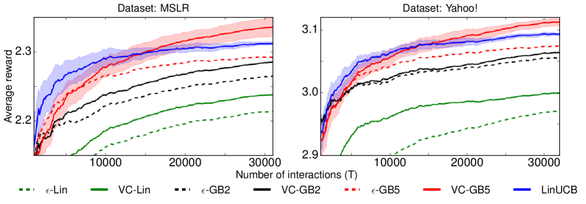
Figure 1: Average reward as a function of number of interactions $T$ for VCEE, $\epsilon$-Greedy, and LinUCB on MSLR (left) and Yahoo (right) learning-to-rank datasets.

Parameter tuning: Each algorithm has a parameter governing the explore-exploit tradeoff. For VCEE, we set $\mu_{t}=c\,\sqrt{1/KLT}$ and tune $c$, in $\epsilon$-Greedy we tune $\epsilon$, and in LinUCB we tune $\alpha$. We ran each algorithm for 10 repetitions, for each of ten logarithmically spaced parameter values.

Results: In Figure 1, we plot the average reward (cumulative reward up to round $t$ divided by $t$) on both datasets. For each $t$, we use the parameter that achieves the best average reward across the 10 repetitions at that $t$. Thus for each $t$, we are showing the performance of each algorithm tuned to maximize reward over $t$ rounds. We found VCEE was fairly stable to parameter tuning, so for VC-GB5 we just use one parameter value ($c=0.008$) for all $t$ on both datasets. We show confidence bands at twice the standard error for just LinUCB and VC-GB5 to simplify the plot.

Qualitatively, both datasets reveal similar phenomena. First, when using the same policy class, VCEE consistently outperforms $\epsilon$-Greedy. This agrees with our theory, as VCEE achieves $\sqrt{T}$-type regret, while a tuned $\epsilon$-Greedy achieves at best a $T^{2/3}$ rate.

Secondly, if we use a rich policy class, VCEE can significantly improve on LinUCB, the empirical state-of-the-art, and one of few practical alternatives to $\epsilon$-Greedy. Of course, since $\epsilon$-Greedy does not outperform LinUCB, the tailored exploration of VCEE is critical. Thus, the combination of these two properties is key to improved performance on these datasets. VCEE is the only contextual semibandit algorithm we are aware of that performs adaptive exploration and is agnostic to the policy representation. Note that LinUCB is quite effective and outperforms VCEE with a linear class. One possible explanation for this behavior is that LinUCB, by directly modeling the reward, searches the policy space more effectively than VCEE, which uses an approximate oracle implementation.

7 Discussion

This paper develops oracle-based algorithms for contextual semibandits both with known and unknown weights. In both cases, our algorithms achieve the best known regret bounds for computationally efficient procedures. Our empirical evaluation of VCEE, clearly demonstrates the advantage of sophisticated oracle-based approaches over both parametric approaches and naive exploration. To our knowledge this is the first detailed empirical evaluation of oracle-based contextual bandit or semibandit learning. We close with some promising directions for future work:

• With known weights, can we obtain $\tilde{O}(\sqrt{KLT\log N})$ regret even with structured action spaces? This may require a new contextual bandit algorithm that does not use uniform smoothing.

• With unknown weights, can we achieve a $\sqrt{T}$ dependence while exploiting semibandit feedback?

Appendix A Analysis of $\epsilon$-Greedy with Known Weights

We analyze the $\epsilon$-greedy algorithm (Algorithm 3) in the known-weights setting when all rankings are valid, i.e., $p_{\textup{min}}=L$. This algorithm is different from the one we use in our experiments in that it is an explore-first variant, exploring for the first several rounds and then exploiting for the remainder. In our experiments, we use a variant where at each round we explore with probability $\epsilon$ and exploit with probability $(1-\epsilon)$. This latter version also has the same regret bound, via an argument similar to that of Langford and Zhang [16].

Algorithm 3 $\epsilon$-Greedy for Contextual Semibandits with Known Weights

0:  Allowed failure probability $\delta\in(0,1)$.

  Set $n=T^{2/3}(K\ln(2N/\delta)/L)^{1/3}$.

  Let $U$ be the uniform distribution over all rankings.

  For $t=1,\ldots,n$, observe $x_{t}$, play $A_{t}\sim U$, observe $y_{t}(A_{t})$ and $r_{t}(A_{t})$.

  Optimize policy $\hat{\pi}\leftarrow\mathop{\mathrm{argmax}}_{\pi\in\Pi}\eta_{n}(\pi,w^{\star})$ using importance-weighted features.

  For every remaining round: observe $x_{t}$, play $A_{t}=\hat{\pi}(x_{t})$.

Theorem 3.

For any $\delta\in(0,1)$, when $T\geq K\ln(N/\delta)/L$, with probability at least $1-\delta$, the regret of Algorithm 3 is at most $\tilde{O}(\|w^{\star}\|_{2}T^{2/3}(K\log(N/\delta))^{1/3}L^{1/6})$.

Proof.

The proof relies on the uniform deviation bound similar to Lemma 20, which we use for the analysis of EELS. We first prove that for any $\delta\in(0,1)$, with probability at least $1-\delta$, for all policies $\pi$, we have

$$|\eta_{n}(\pi,w^{\star})-\mathcal{R}(\pi)|\leq\lVert w^{\star}\rVert_{2}\left(\sqrt{\frac{2K\ln(2N/\delta)}{n}}+\frac{2K}{3\sqrt{L}}\frac{\ln(2N/\delta)}{n}\right).$$ (6)

This deviation bound is a consequence of Bernstein’s inequality. The quantity on the left-hand side is the average of $n$ terms

$$\hat{y}_{i}(\pi(x_{i}))^{T}w^{\star}-\mathbb{E}_{x,y}[y(\pi(x))]^{T}w^{\star},$$

all with expectation zero, because $\hat{y}$ is unbiased. The range of each term is bounded by the Cauchy-Schwarz inequality as

$$\|w^{\star}\|_{2}\|\hat{y}_{i}(\pi(x_{i}))-\mathbb{E}_{x,y}[y(\pi(x))]\|_{2}\leq\|w^{\star}\|_{2}K/\sqrt{L},$$

because under uniform exploration the coordinates of $\hat{y}_{i}(\pi(x_{i}))$ are bounded in $[0,K/L]$ while the coordinates of $y(\pi(x))$ are in $[0,1]$ and these are $L$-dimensional vectors. The variance is bounded by the second moment, which we bound as follows:

$$\mathbb{E}_{x,y,A}\left[(\hat{y}(\pi(x))^{T}w^{\star})^{2}\right] \leq\|w^{\star}\|_{2}^{2}\,\mathbb{E}_{x,y,A}\!\left[\sum_{l=1}^{L}\hat{y}(\pi(x_{l}))^{2}\right]$$

$$\leq\|w^{\star}\|_{2}^{2}\,\mathbb{E}_{x,y,A}\!\left[\sum_{l=1}^{L}\frac{K^{2}}{L^{2}}\mathbf{1}(\pi(x)_{l}\in A)\right]=\|w^{\star}\|^{2}K,$$

since $\mathbb{E}_{x,y,A}[\mathbf{1}(\pi(x)_{l}\in A)]=L/K$ under uniform exploration. Plugging these bounds into Bernstein’s inequality gives the deviation bound of Eq. (6).

Now we can prove the theorem. Eq. (6) ensures that after collecting $n$ samples, the expected reward of the empirical reward maximizer $\hat{\pi}$ is close to $\max_{\pi}\mathcal{R}(\pi)$, the best achievable reward. The difference between these two is at most twice the right-hand side of the deviation bound. If we perform uniform exploration for $n$ rounds, we are ensured that with probability at least $1-\delta$ the regret is at most

Regret $$\leq n\|w^{\star}\|_{2}\sqrt{L}+2(T-n)\|w^{\star}\|_{2}\left(\sqrt{\frac{2K\ln(2N/\delta)}{n}}+\frac{2K}{3\sqrt{L}}\frac{\ln(2N/\delta)}{n}\right)$$

$$\leq n\|w^{\star}\|_{2}\sqrt{L}+3T\|w^{\star}\|_{2}\left(\sqrt{\frac{K\ln(2N/\delta)}{n}}+\frac{K}{\sqrt{L}}\frac{\ln(2N/\delta)}{n}\right).$$

For our setting of $n=T^{2/3}(K\ln(2N/\delta)/L)^{1/3}$, the bound is

$$4\|w^{\star}\|_{2}T^{2/3}(K\ln(2N/\delta))^{1/3}L^{1/6}+3\|w^{\star}\|_{2}T^{1/3}(K\ln(2N/\delta))^{2/3}L^{-1/6}.$$

Under the assumption on $T$, the second term is lower order, which proves the result. ∎

Appendix B Comparisons for EELS

In this section we do a detailed comparison of our Theorem 2 to the paper of Swaminathan et al. [24], which is the most directly applicable result. We use notation consistent with our paper.

Swaminathan et al. [24] focus on off-policy evaluation in a more challenging setting where no semibandit feedback is provided. Specifically, in their setting, in each round, the learner observes a context $x\in\mathcal{X}$, chooses a composite action $A$ (as we do here) and receives reward $r(A)\in[-1,1]$. They assume that the reward decomposes linearly across the action-position pairs as

$$\mathbb{E}[r(A)|x,A]=\sum_{\ell=1}^{L}\phi_{x}(a_{\ell},\ell).$$

With this assumption, and when exploration is done uniformly, they provide off-policy reward estimation bounds of the form

$$|\eta_{n}(\pi)-\mathcal{R}(\pi)|\leq O\left(\sqrt{\frac{KL\ln(1/\delta)}{n}}\right).$$

This bound holds for any policy $\pi:\mathcal{X}\rightarrow\mathcal{A}^{L}$ with probability at least $1-\delta$ for any $\delta\in(0,1)$. (See Theorem 3 and the following discussion in Swaminathan et al. [24].) Note that this assumption generalizes our unknown weights setting, since we can always define $\phi_{x}(a,j)=w^{\star}_{j}y(a)$.

To do an appropriate comparison, we first need to adjust the scaling of the rewards. While Swaminathan et al. [24] assume that rewards are bounded in $[-1,1]$, we only assume bounded $y$’s and bounded noise. Consequently, we need to adjust their bound to incorporate this scaling. If the rewards are scaled to lie in $[-R,R]$, their bound becomes

$$|\eta_{n}(\pi)-\mathcal{R}(\pi)|\leq O\left(R\sqrt{\frac{KL\ln(1/\delta)}{n}}\right).$$

This deviation bound can be turned into a low-regret algorithm by exploring for the first $n$ rounds, finding an empirically best policy, and using that policy for the remaining $T-n$ rounds. Optimizing the bound in $n$ leads to a $T^{2/3}$-style regret bound:

Fact 4.

The approach of Swaminathan et al. [24] with rewards in $[-R,R]$ leads to an algorithm with regret bound

$$O\left(RT^{2/3}(KL\log N)^{1/3}\right).$$

This algorithm can be applied as is to our setting, so it is worth comparing it to EELS. According to Theorem 2, EELS has a regret bound

$$O\left(T^{2/3}(K\log N)^{1/3}\max\{B^{1/3}L^{1/2},BL^{1/6}\}\right).$$

The dependence on $T,K$, and $\log N$ match between the two algorithms, so we are left with $L$ and the scale factors $B,R$. This comparison is somewhat subtle and we use two different arguments. The first finds a conservative value for $R$ in Fact 4 in terms of $B$ and $L$. This is the regret bound one would obtain by using the approach of Swaminathan et al. [24] in our precise setting, ignoring the semibandit feedback, but with known weight-vector bound $B$. The second comparison finds a conservative value of $B$ in terms of $R$ and $L$.

For the first comparison, recall that our setting makes no assumptions on the scale of the reward, except that the noise $\xi$ is bounded in $[-1,1]$, so our setting never admits $R<1$. If we begin with a setting of $B$, we need to conservatively set $R=\max\{B\sqrt{L},1\}$, which gives the dependence

$$\text{EELS: }\max\{B^{1/3}L^{1/2},BL^{1/6}\}$$

$$\text{\cite[citet]{\@@bibref{Authors Phrase1NumberPhrase2}{swaminathan2016off}{\@@citephrase{[}}{\@@citephrase{]}}}: }\max\{BL^{5/6},L^{1/3}\}.$$

The EELS bound is never worse than the bound in Fact 4 according to this comparison. At $B=\Theta(L^{-1/2})$, the two bounds are of the same order, which is $\Theta(L^{1/3})$. For $B=O(L^{-1/2})$, the EELS bound is at most $L^{1/3}$, while for $B=\Omega(L^{-1/2})$ the first term in the EELS bound is at most the first term in the Swaminathan et al. [24] bound. In both cases, the EELS bound is superior. Finally when $B=\Omega(\sqrt{L})$, the second term dominates our bound, so EELS demonstrates an $L^{2/3}$ improvement.

For the second comparison, since our setting has the noise bounded in $[-1,1]$, assume that $R\geq 1$ and that the total reward is scaled in $[-R,R]$ as in Fact 4. If we want to allow any $y(A)\in[0,1]^{L}$, the tightest setting of $R$ is between $\lVert w^{\star}\rVert_{1}/2$ and $\lVert w^{\star}\rVert_{1}$ (depending on the structure of the positive and negative coordinates of $w^{\star}$). For simplicity, assume $R$ is a bound on $\lVert w^{\star}\rVert_{1}$. Since the EELS bound depends on $B$, a bound on the Euclidean norm of $w^{\star}$, we use $\lVert w^{\star}\rVert_{2}\leq\lVert w^{\star}\rVert_{1}\leq\sqrt{L}\lVert w^{\star}\rVert_{2}$ to obtain a conservative setting of $B=R$. This gives the dependence

$$\text{EELS: }\max\{R^{1/3}L^{1/2},RL^{1/6}\}$$

$$\text{\cite[citet]{\@@bibref{Authors Phrase1NumberPhrase2}{swaminathan2016off}{\@@citephrase{[}}{\@@citephrase{]}}}: }RL^{1/3}$$

Since $R\geq 1$, the EELS bound is superior whenever $R\geq L^{1/4}$. Moreover, if $R=\Omega({\sqrt{L}})$, i.e., at least $\sqrt{L}$ positions are relevant, the second term dominates our bound, and we improve by a factor of $L^{1/6}$. The EELS bound is inferior when $R\leq L^{1/4}$, which corresponds to a high-sparsity case since $R$ is also a bound on $\lVert w^{\star}\rVert_{1}$ in this comparison.

Appendix C Implementation Details

C.1 Implementation of VCEE

VCEE is implemented as stated in Algorithm 1 with some modifications, primarily to account for an imperfect oracle. OP is solved using the coordinate descent procedure described in Appendix E.

We set $\psi=1$ in our implementation and ignore the log factor in $\mu_{t}$. Instead, since $p_{\textup{min}}=L$, we use $\mu_{t}=c\sqrt{1/KLT}$ and tune $c$, which can compensate for the absence of the $\log(t^{2}N/\delta)$ factor. This additionally means that we ignore the failure probability parameter $\delta$. Otherwise, all other parameters and constants are set as described in Algorithm 1 and OP.

As mentioned in Section 6, we implement AMO via a reduction to squared loss regression. There are many possibilities for this reduction. In our case, we specify a squared loss regression problem via a dataset $D=\{x_{i},A_{i},y_{i},\gamma_{i}\}_{i=1}^{n}$ where $x_{i}\in\mathcal{X}$, $A_{i}$ is any list of actions, $y_{i}\in\mathbb{R}^{K}$ assigns a value to each action, and $\gamma_{i}\in\mathbb{R}^{K}$ assigns an importance weight to each action. Since in our experiments $w^{\star}=\mathbf{1}$, we do not need to pass along the vectors $v_{i}\in\mathbb{R}^{L}$ described in Eq. (2).

Given such a dataset $D$, we minimize a weighted squared loss objective over a regression class $\mathcal{F}$,

$$\hat{f}=\mathop{\mathrm{argmin}}_{f\in\mathcal{F}}\sum_{i=1}^{n}\sum_{a\in A_{i}}\gamma_{i}(a)(f(\phi(x_{i},a))-y_{i}(a))^{2},$$ (7)

where $\phi(x,a)$ is a feature vector associated with the given query-document pair. Note that we only include terms corresponding to simple actions in $A_{i}$ for each $i$. This regression function is associated with the greedy policy that chooses the best valid ranking according to the sum of rewards of individual actions as predicted by $\hat{f}$ on the current context.

We access this oracle with two different kinds of datasets. When we access AMO to find the empirically best policy, we only use the history of the interaction. In this case, we only regress onto the chosen actions in the history and we let $\gamma_{i}$ be their importance weights. More formally, suppose that at round $t$, we observe context $x_{t}$, choose composite action $A_{t}\sim q_{t}$ and receive feedback $\{y_{t}(a_{t,\ell})\}_{\ell=1}^{L}$. We create a single example $(x_{t},A_{t},z_{t},\gamma_{t})$ where $x_{t}$ is the context, $A_{t}$ is the chosen composite action, $z_{t}$ has $z_{t}(a)=\mathbf{1}(a\in A_{t})y_{t}(a)$ and $\gamma_{t}(a)=1/q_{t}(a\in A_{t})$. Observe that when this sample is passed into Eq. (7), it leads to a different objective than if we regressed directly onto the importance-weighted reward features $\hat{y}_{t}$.

We also create datasets to verify the variance constraint within OP. For this, we use the AMO in a more direct way by setting $A_{t}$ to be a list of all $K$ actions, letting $y_{t}$ be the importance weighted vector, and $\gamma_{t}=\mathbf{1}$.

We use this particular implementation because leaving the importance weights inside the square loss term introduces additional variance, which we would like to avoid.

The imperfect oracle introduces one issue that needs to be corrected. Since the oracle is not guaranteed to find the maximizing policy on every dataset, in the $t$th round of the algorithm, we may encounter a policy $\pi$ that has $\widehat{\textup{Reg}}_{t}(\pi)<0$, which can cause the coordinate descent procedure to loop indefinitely. Of course, if we ever find a policy $\pi$ with $\widehat{\textup{Reg}}_{t}(\pi)<0$, it means that we have found a better policy, so we simply switch the leader. We found that with this intuitive change, the coordinate descent procedure always terminates in a few iterations.

C.2 Implementation of $\epsilon$-Greedy

Recall that we run a variant of $\epsilon$-Greedy where at each round we explore with probability $\epsilon$ and exploit with probability $(1-\epsilon)$, which is slightly different from the explore-first algorithm analyzed in Appendix A.

For $\epsilon$-Greedy, we also use the oracle defined in Eq. (7). This algorithm only accesses the oracle to find the empirically best policy, and we do this in the same way as VCEE does, i.e., we only regress onto actions that were actually selected with importance weights encoded via $\gamma_{i}$s. We use all of the data, including the data from exploitation rounds, with importance weighting.

C.3 Implementation of LinUCB

The semibandit version of LinUCB uses ridge regression to predict the semibandit feedback given query-document features $\phi(x,a)$. If the feature vectors are in $d$ dimensions, we start with $\Sigma_{1}=I_{d}$ and $\theta_{1}=0$, the all zeros vector. At round $t$, we receive the query-document feature vectors $\{\phi(x_{t},a)\}_{a\in\mathcal{A}}$ for query $x_{t}$ and we choose

$$A_{t}=\mathop{\mathrm{argmax}}_{A}\left\{\sum_{a\in A}\theta_{t}^{T}\phi(x_{t},a)+\alpha\phi(x_{t},a)^{T}\Sigma_{t}^{-1}\phi(x_{t},a)\right\}.$$

Since in our experiment we know that $w^{\star}=\mathbf{1}$ and all rankings are valid, the order of the documents is irrelevant and the best ranking consists of the top $L$ simple actions with the largest values of the above “regularized score”. Here $\alpha$ is a parameter of the algorithm that we tune.

After selecting a ranking, we collect the semibandit feedback $\{y_{t}(a_{t,\ell})\}_{\ell=1}^{L}$. The standard implementation would perform the update

$$\Sigma_{t+1} \leftarrow\Sigma_{t}+\sum_{\ell=1}^{L}\phi(x_{t},a_{t,\ell})\phi(x_{t},a_{t,\ell})^{T},\qquad\theta_{t+1}\leftarrow\Sigma_{t+1}^{-1}\left(\sum_{i=1}^{t}\sum_{\ell=1}^{L}\phi(x_{i},a_{i,\ell})y_{i}(a_{i,\ell})\right),$$

which is the standard online ridge regression update. For computational reasons, we only update every 100 iterations, using all of the data. Thus, if $\textrm{mod}(t,100)\neq 0$, we set $\Sigma_{t+1}\leftarrow\Sigma_{t}$ and $\theta_{t+1}\leftarrow\theta_{t}$. If $\textrm{mod}(t,100)=0$, we set

$$\Sigma_{t+1} \leftarrow I+\sum_{i=1}^{t}\sum_{\ell=1}^{L}\phi(x_{i},a_{i,\ell})\phi(x_{i},a_{i,\ell})^{T},\qquad\theta_{t+1}\leftarrow\Sigma_{t+1}^{-1}\left(\sum_{i=1}^{t}\sum_{\ell=1}^{L}\phi(x_{i},a_{i,\ell})y_{i}(a_{i,\ell})\right).$$

C.4 Policy Classes

As AMO for both VCEE and $\epsilon$-Greedy, we use the default implementations of regression with various function classes in scikit-learn version 0.17. We instantiate scikit-learn model objects and use the fit() and predict() routines. The model objects we use are

• sklearn.linear_model.LinearRegression()

• sklearn.ensemble.GradientBoostingRegressor(n_estimators=50,max_depth=2)

• sklearn.ensemble.GradientBoostingRegressor(n_estimators=50,max_depth=5)

All three objects accommodate weighted least-squares objectives as required by Eq. (7).

Appendix D Proof of Regret Bound in Theorem 1

The proof hinges on two uniform deviation bounds, and then a careful inductive analysis of the regret using the OP. We only need our two deviation bounds to hold for the rounds $t$ in which $\mu_{t}=\sqrt{\ln(16t^{2}N/\delta)/(Ktp_{\textup{min}})}$. Let $d_{t}\coloneqq\ln(16t^{2}N/\delta)$. These rounds then start at

$$t_{0}\coloneqq\min\left\{t:\>\sqrt{\frac{d_{t}}{Ktp_{\textup{min}}}}\leq\frac{1}{2K}\right\}=\min\left\{t:\>\frac{d_{t}}{t}\leq\frac{p_{\textup{min}}}{4K}\right\}.$$

Note that $t_{0}\geq 4$ since $d_{t}\geq 1$ and $K\geq p_{\textup{min}}$. From the definition of $t_{0}$, we have for all $t\geq t_{0}$:

$$\mu_{t}\geq\sqrt{d_{t}/(Ktp_{\textup{min}})},\quad t\geq 4Kd_{t}/p_{\textup{min}}.$$ (8)

The first deviation bound shows that the variance estimates used in Eq. (5) are suitable estimators for the true variance of the distribution. To state this deviation bound, we need some definitions:

$$V(P,\pi,\mu)\coloneqq\mathbb{E}_{x\sim\mathcal{D}_{x}}\left[\sum_{\ell=1}^{L}\frac{1}{P^{\mu}(\pi(x)_{\ell}\mathbin{|}x)}\right],\quad\hat{V}_{t}(P,\pi,\mu)\coloneqq\hat{\mathbb{E}}_{x\sim H_{t}}\left[\sum_{\ell=1}^{L}\frac{1}{P^{\mu}(\pi(x)_{\ell}\mathbin{|}x)}\right].$$ (9)

In these definitions and throughout this appendix we use the shorthand $P(a\mathbin{|}x)$ to mean $P(a\in A\mathbin{|}x)$ for any projected subdistribution $P(A\mathbin{|}x)$. If $P$ is a distribution, we have $\sum_{a\in\mathcal{A}}P(a\mathbin{|}x)=L$. For a subdistribution, this sum can be smaller, so $\sum_{a\in\mathcal{A}}P(a\mathbin{|}x)\leq L$ for all subdistributions. The deviation bound is in the following theorem:

Theorem 5.

Let $\delta\in(0,1)$. Then with probability at least $1-\delta/8$, for all $t\geq t_{0}$, all distributions $P$ over $\Pi$, and all $\pi\in\Pi$, we have

$$V(P,\pi,\mu_{t})\leq 6.4\hat{V}_{t}(P,\pi,\mu_{t})+81.3\frac{KL}{p_{\textup{min}}}.$$ (10)

Proof.

The proof of this theorem is similar to a related result of Agarwal et al. [1] (See their Lemma 10). We first use Freedman’s inequality (Lemma 23) to argue that for a fixed $P,\pi,\mu$, and $t$, the empirical version of the variance is close to the true variance. We then use a discretization of the set of all distributions and take a union bound to extend this deviation inequality to all $P,\pi,\mu,t$.

To start, we have:

Lemma 6.

For fixed $P,\pi,\mu,t$ and for any $\lambda\in\left[0,\frac{\mu p_{\textup{min}}}{L}\right]$, with probability at least $1-\delta$:

$$V(P,\pi,\mu)-\hat{V}_{t}(P,\pi,\mu)\leq\frac{(e-2)\lambda L}{\mu p_{\textup{min}}}V(P,\pi,\mu)+\frac{\ln(1/\delta)}{t\lambda}$$

Proof.

Let:

$$Z_{i}\coloneqq\sum_{\ell=1}^{L}\frac{1}{P^{\mu}(\pi(x_{i})_{\ell}|x_{i})}-\mathbb{E}_{x\sim\mathcal{D}_{x}}\sum_{\ell=1}^{L}\frac{1}{P^{\mu}(\pi(x)_{\ell}|x)},$$

and notice that $\frac{1}{t}\sum_{i=1}^{t}Z_{i}=\hat{V}_{t}(P,\pi,\mu)-V(P,\pi,\mu)$. Clearly, $\mathbb{E}Z_{i}=0$ for all $i$ and $\max_{i}|Z_{i}|\leq L/\mu p_{\textup{min}}$ since when we smooth by $\mu$, each simple action that $\pi$ could choose must appear with probability at least $\mu p_{\textup{min}}$. By the Cauchy-Schwarz and Holder inequalities, the conditional variance is:

$$\mathbb{E}_{x\sim\mathcal{D}_{x}}Z_{i}^{2} \leq\mathbb{E}_{x\sim\mathcal{D}_{x}}\left(\sum_{\ell=1}^{L}\frac{1}{P^{\mu}(\pi(x)_{\ell}|x)}\right)^{2}\leq L\mathbb{E}_{x\sim\mathcal{D}_{x}}\sum_{\ell=1}^{L}\frac{1}{P^{\mu}(\pi(x)_{\ell}|x)^{2}}$$

$$\leq\frac{L}{\mu p_{\textup{min}}}\mathbb{E}_{x\sim\mathcal{D}_{x}}\sum_{\ell=1}^{L}\frac{1}{P^{\mu}(\pi(x)_{\ell}|x)}=\frac{L}{\mu p_{\textup{min}}}V(P,\pi,\mu).$$

The lemma now follows by Freedman’s inequality. ∎

To prove the variance deviation bound of Theorem 5, we next use a discretization lemma from [10] (their Lemma 16) which immediately implies that for any $P$, there exists a distribution $P^{\prime}$ supported on at most $N_{t}$ policies such that for $c_{t}>0$, if $N_{t}\geq\frac{6}{\gamma_{t}^{2}\mu_{t}p_{\textup{min}}}$:

$$V(P,\pi,\mu)-V(P^{\prime},\pi,\mu_{t})+c_{t}\left(\hat{V}_{t}(P^{\prime},\pi,\mu_{t})-\hat{V}_{t}(P,\pi,\mu_{t})\right)\leq\gamma_{t}(V(P,\pi,\mu_{t})+c_{t}\hat{V}_{t}(P,\pi,\mu_{t}))$$

This is exactly the second conclusion of their Lemma 16 except we use $c_{t}$ instead of their $(1+\lambda)$ (we will set $c_{t}>1$). The other difference is the inclusion of $p_{\textup{min}}$ in the lower bound on $N_{t}$, which is based on a straightforward modification to their proof.

We set $\gamma_{t}=\sqrt{\frac{1-K\mu_{t}}{N_{t}\mu_{t}p_{\textup{min}}}}+3\frac{1-K\mu_{t}}{N_{t}\mu_{t}p_{\textup{min}}},c_{t}=\frac{1}{1-\frac{(e-2)L\lambda_{t}}{\mu_{t}p_{\textup{min}}}},N_{t}=\lceil\frac{12(1-K\mu_{t})}{\mu_{t}p_{\textup{min}}}\rceil$ and $\lambda_{t}=0.66\mu_{t}p_{\textup{min}}/L$. The choice of $c_{t}$ is motivated by Lemma 6, which can be rearranged to (for a distribution $P^{\prime}$)

$$\ V(P^{\prime},\pi,\mu_{t})-\frac{1}{1-\frac{(e-2)L\lambda_{t}}{\mu_{t}p_{\textup{min}}}}\hat{V}_{t}(P^{\prime},\pi,\mu_{t})\leq\frac{1}{1-\frac{(e-2)L\lambda_{t}}{\mu_{t}p_{\textup{min}}}}\frac{\ln(1/\delta)}{t\lambda_{t}}$$

$$\Leftrightarrow\ V(P^{\prime},\pi,\mu_{t})-c_{t}\hat{V}_{t}(P^{\prime},\pi,\mu_{t})\leq c_{t}\frac{\ln(1/\delta)}{t\lambda_{t}}.$$

To take a union over all $t\in\mathbb{N}$, $N_{t}$-point distributions $P$ over $\Pi$, and all $\pi\in\Pi$, we set $\delta_{t}=\delta(\frac{1}{2t^{2}N^{N_{t}+1}})$ in the $t$th iteration. This inequality becomes

$$V(P^{\prime},\pi,\mu_{t})-c_{t}\hat{V}_{t}(P^{\prime},\pi,\mu_{t})\leq c_{t}\frac{\ln(2N^{N_{t}+1}t^{2}/\delta)}{t\lambda_{t}}.$$

The choice of $c_{t}$ and $\lambda_{t}$ leads to a bound $c_{t}=\frac{1}{1-0.66(e-2)}\leq 1.91$.

We also use the values of $N_{t}$ and $\gamma_{t}$ to bound

$$\gamma_{t}=\sqrt{\frac{1-K\mu_{t}}{N_{t}\mu_{t}p_{\textup{min}}}}+3\frac{1-K\mu_{t}}{N_{t}\mu_{t}p_{\textup{min}}}\leq\sqrt{\frac{1}{12}}+\frac{1}{4}.$$

Rearranging the discretization claim gives

$$V(P,\pi,\mu_{t}) \leq\frac{c_{t}(1+\gamma_{t})}{(1-\gamma_{t})}\hat{V}_{t}(P,\pi,\mu_{t})+\frac{1}{(1-\gamma_{t})}\left(V(P^{\prime},\pi,\mu_{t})-c_{t}\hat{V}_{t}(P^{\prime},\pi,\mu_{t})\right)$$

$$\leq 6.4\hat{V}_{t}(P,\pi,\mu_{t})+\frac{c_{t}}{(1-\gamma_{t})}\frac{\ln(2N^{N_{t}+1}t^{2}/\delta)}{t\lambda_{t}}.$$

Using the bounds on $c_{t},\gamma_{t}$ and the settings of $N_{t}$ and $\lambda_{t}$, this last term is at most

$$\frac{c_{t}}{(1-\gamma_{t})}\left(\frac{L\ln(2N^{2}t^{2}/\delta)}{t\mu_{t}p_{\textup{min}}}+\frac{LN_{t}\ln(N)}{t\mu_{t}p_{\textup{min}}}\right)\leq\frac{6.3L\ln(16N^{2}t^{2}/\delta)}{\mu_{t}tp_{\textup{min}}}+\frac{75L(1-K\mu_{t})\ln(N)}{\mu_{t}^{2}tp_{\textup{min}}^{2}}.$$

The theorem now follows from the bounds of Eq. (8). ∎

The other main deviation bound is a straightforward application of Freedman’s inequality and a union bound. To state the lemma, we must introduce one more definition. Let

$$\mathcal{V}_{t}(\pi)\coloneqq\max_{0\leq\tau\leq t-1}V(\tilde{Q}_{\tau},\pi,\mu_{\tau})$$

where $\tilde{Q}_{\tau}$ is the distribution calculated in Step 3 of Algorithm 1. Note that $\tilde{Q}^{\mu_{\tau}}_{\tau}$ is the distribution used to select the composite action in round $\tau+1$.

Lemma 7.

Let $\delta\in(0,1)$. Then with probability at least $1-\delta/4$, for all $t\geq t_{0}$ and $\pi\in\Pi$, we have

$$|\eta_{t}(\pi,w^{\star})-\mathcal{R}(\pi)|\leq\frac{\lVert w^{\star}\rVert_{2}^{2}}{\lVert w^{\star}\rVert_{1}}\mathcal{V}_{t}(\pi)p_{\textup{min}}\mu_{t}+\frac{\lVert w^{\star}\rVert_{2}^{2}}{\lVert w^{\star}\rVert_{1}}KL\mu_{t}.$$ (11)

Proof.

Consider a specific $t\geq t_{0}$ and $\pi\in\Pi$. Let

$$Z_{i}\coloneqq\langle w^{\star},\hat{y}_{i}(\pi(x_{i}))\rangle-\langle w^{\star},y_{i}(\pi(x_{i}))\rangle$$

and note that $\frac{1}{t}\sum_{i=1}^{t}Z_{i}=\eta_{t}(\pi,w^{\star})-\mathcal{R}(\pi)$. Since $\hat{y}_{i}$ is an unbiased estimate of $y_{i}$, the $Z_{i}$s form a martingale. The range of each $Z_{i}$ is bounded as

$$\lvert Z_{i}\rvert\leq\lVert w^{\star}\rVert_{1}\lVert\hat{y}_{i}-y_{i}\rVert_{\infty}\leq\frac{\lVert w^{\star}\rVert_{1}}{\mu_{i-1}p_{\textup{min}}}\leq\frac{\lVert w^{\star}\rVert_{1}}{\mu_{t}p_{\textup{min}}},$$

because the $\mu_{i}$s are non-increasing. The conditional variance can be bounded via the Cauchy-Schwarz inequality:

$$\mathbb{E}[Z_{i}^{2}\mathbin{|}H_{i-1}] \leq\|w^{\star}\|_{2}^{2}\sum_{\ell=1}^{L}\mathbb{E}_{x\sim\mathcal{D}_{x}}\mathbb{E}_{y\mathbin{|}x}\frac{y(\pi(x)_{\ell})^{2}}{\tilde{Q}^{\mu_{i-1}}_{i-1}(\pi(x)_{\ell}\mathbin{|}x)}$$

$$\leq\|w^{\star}\|_{2}^{2}V(\tilde{Q}_{i-1},\pi,\mu_{i-1})\leq\|w^{\star}\|_{2}^{2}\mathcal{V}_{t}(\pi).$$

By Freedman’s inequality with $\lambda=\mu_{t}p_{\textup{min}}/\lVert w^{\star}\rVert_{1}$, we have, with probability at least $1-\delta/(8t^{2}N)$,

$$|\eta_{t}(\pi,w^{\star})-\mathcal{R}(\pi)| \leq\frac{\mu_{t}p_{\textup{min}}}{\lVert w^{\star}\rVert_{1}}\cdot\lVert w^{\star}\rVert_{2}^{2}\mathcal{V}_{t}(\pi)+\frac{d_{t}}{t}\cdot\frac{\lVert w^{\star}\rVert_{1}}{\mu_{t}p_{\textup{min}}}$$

$$\leq\frac{\lVert w^{\star}\rVert_{2}^{2}}{\lVert w^{\star}\rVert_{1}}\mathcal{V}_{t}(\pi)p_{\textup{min}}\mu_{t}+K\mu_{t}\lVert w^{\star}\rVert_{1}$$ (12)

$$\leq\frac{\lVert w^{\star}\rVert_{2}^{2}}{\lVert w^{\star}\rVert_{1}}\mathcal{V}_{t}(\pi)p_{\textup{min}}\mu_{t}+\frac{\lVert w^{\star}\rVert_{2}^{2}}{\lVert w^{\star}\rVert_{1}}KL\mu_{t}.$$ (13)

Here, Eq. (12) follows because $d_{t}/(p_{\textup{min}}t)\leq K\mu_{t}^{2}$ by Eq. (8). Eq. (13) follows because $\lVert w^{\star}\rVert_{1}\leq L\lVert w^{\star}\rVert_{2}^{2}/\lVert w^{\star}\rVert_{1}$ by the fact that $\lVert w^{\star}\rVert_{1}\leq\sqrt{L}\lVert w^{\star}\rVert_{2}$. The lemma follows by a union bound over all $t\geq t_{0}$ and $\pi\in\Pi$. ∎

Equipped with these two deviation bounds we will proceed to prove the main theorem. Let $\mathcal{E}$ denote the event that both the variance and reward deviation bounds of Theorem 5 and Lemma 7 hold. Note that $\mathbb{P}(\mathcal{E})\geq 1-\delta/2$. Using the variance constraint, it is straightforward to prove the following lemma:

Lemma 8.

Assume event $\mathcal{E}$ holds, then for any round $t\geq 1$ and any policy $\pi\in\Pi$, let $t_{\star}$ be the round achieving the $\max$ in the definition of $\mathcal{V}_{t}(\pi)$. Then there are universal constants $\theta_{1}\geq 2$ and $\theta_{2}$ such that:

$$\mathcal{V}_{t}(\pi)\leq\begin{cases}\displaystyle\frac{2KL}{p_{\textup{min}}}&\text{if $t_{\star}<t_{0}$,}\\[12.0pt] \displaystyle\frac{\theta_{1}KL}{p_{\textup{min}}}+\frac{\|w^{\star}\|_{1}}{\|w^{\star}\|_{2}^{2}}\frac{\widehat{\textup{Reg}}_{t_{\star}}(\pi)}{\theta_{2}p_{\textup{min}}\mu_{t_{\star}}}&\text{if $t_{\star}\geq t_{0}$.}\end{cases}$$ (14)

Proof.

The first claim follows by the definition of $\mathcal{V}_{t}(\pi)$ and the fact that $\mu_{\tau}=1/2K$ for $\tau<t_{0}$. For the second claim, we use the variance deviation bound and the optimization constraint. In particular, since $t_{\star}\geq t_{0}$, we can apply Theorem 5:

$$V(\tilde{Q}_{t_{\star}},\pi,\mu_{t_{\star}})\leq 6.4\hat{V}_{t_{\star}}(\tilde{Q}_{t_{\star}},\pi,\mu_{t_{\star}})+81.3\frac{KL}{p_{\textup{min}}},$$

and we can use the optimization constraint which gives an upper bound on $\hat{V}_{t_{\star}}(\tilde{Q}_{t_{\star}},\pi,\mu_{t_{\star}})$:

$$\hat{V}_{t_{\star}}(\tilde{Q}_{t_{\star}},\pi,\mu_{t_{\star}})\leq\hat{V}_{t_{\star}}(Q_{t_{\star}},\pi,\mu_{t_{\star}})\leq\frac{2KL}{p_{\textup{min}}}+\frac{\|w^{\star}\|_{1}}{\|w^{\star}\|_{2}^{2}}\frac{\widehat{\textup{Reg}}_{t_{\star}}(\pi)}{\psi p_{\textup{min}}\mu_{t_{\star}}}$$

The bound follows by the choice $\theta_{1}=94.1$ and $\theta_{2}=\psi/6.4$. ∎

We next compare $\textup{Reg}(\pi)$ and $\widehat{\textup{Reg}}(\pi)$ using the variance bounds above.

Lemma 9.

Assume event $\mathcal{E}$ holds and define $c_{0}\coloneqq 4(1+\theta_{1})$. For all $t\geq t_{0}$ and all policies $\pi\in\Pi$:

$$\textup{Reg}(\pi)\leq 2\widehat{\textup{Reg}}_{t}(\pi)+c_{0}\frac{\lVert w^{\star}\rVert_{2}^{2}}{\lVert w^{\star}\rVert_{1}}KL\mu_{t}\quad\mbox{and}\quad\widehat{\textup{Reg}}_{t}(\pi)\leq 2\textup{Reg}(\pi)+c_{0}\frac{\lVert w^{\star}\rVert_{2}^{2}}{\lVert w^{\star}\rVert_{1}}KL\mu_{t}.$$ (15)

Proof.

The proof is by induction on $t$. As the base case, consider $t=t_{0}$ where we have $\mu_{\tau}=1/(2K)$ for all $\tau<t_{0}$, so $\mathcal{V}_{t}(\pi)\leq 2KL/p_{\textup{min}}$ for all $\pi\in\Pi$ by Lemma 8. Using the reward deviation bound of Lemma 7, which holds under $\mathcal{E}$, we thus have

$$|\eta_{t}(\pi,w^{\star})-\mathcal{R}(\pi)|\leq\frac{\lVert w^{\star}\rVert_{2}^{2}}{\lVert w^{\star}\rVert_{1}}\mathcal{V}_{t}(\pi)p_{\textup{min}}\mu_{t}+\frac{\lVert w^{\star}\rVert_{2}^{2}}{\lVert w^{\star}\rVert_{1}}KL\mu_{t}\leq 3\frac{\lVert w^{\star}\rVert_{2}^{2}}{\lVert w^{\star}\rVert_{1}}KL\mu_{t}$$

for all $\pi\in\Pi$. Now both directions of the bound follow from the triangle inequality and the optimality of $\pi_{t}$ for $\eta_{t}(\cdot)$ and $\pi_{\star}$ for $\mathcal{R}(\cdot)$, using the fact that $c_{0}\geq 6$ from the definition of $\theta_{1}$.

For the inductive step, fix some round $t$ and assume that the claim holds for all $t_{0}\leq t^{\prime}<t$ and all $\pi\in\Pi$. By the optimality of $\pi_{t}$ for $\eta_{t}$ and Lemma 7, we have

$$\textup{Reg}(\pi)-\widehat{\textup{Reg}}_{t}(\pi) =(\mathcal{R}(\pi_{\star})-\mathcal{R}(\pi))-(\eta_{t}(\pi_{t},w^{\star})-\eta_{t}(\pi,w^{\star}))$$

$$\leq(\mathcal{R}(\pi_{\star})-\mathcal{R}(\pi))-(\eta_{t}(\pi_{\star},w^{\star})-\eta_{t}(\pi,w^{\star}))$$

$$\leq(\mathcal{V}_{t}(\pi_{\star})+\mathcal{V}_{t}(\pi))\frac{\lVert w^{\star}\rVert_{2}^{2}}{\lVert w^{\star}\rVert_{1}}p_{\textup{min}}\mu_{t}+2\frac{\lVert w^{\star}\rVert_{2}^{2}}{\lVert w^{\star}\rVert_{1}}KL\mu_{t}.$$

Now by Lemma 8, there exist rounds $i,j<t$ such that

$$\mathcal{V}_{t}(\pi) \leq\frac{\theta_{1}KL}{p_{\textup{min}}}+\frac{\|w^{\star}\|_{1}}{\|w^{\star}\|_{2}^{2}}\frac{\widehat{\textup{Reg}}_{i}(\pi)}{\theta_{2}p_{\textup{min}}\mu_{i}}\mathbf{1}(i\geq t_{0})$$

$$\mathcal{V}_{t}(\pi_{\star}) \leq\frac{\theta_{1}KL}{p_{\textup{min}}}+\frac{\|w^{\star}\|_{1}}{\|w^{\star}\|_{2}^{2}}\frac{\widehat{\textup{Reg}}_{j}(\pi_{\star})}{\theta_{2}p_{\textup{min}}\mu_{j}}\mathbf{1}(j\geq t_{0})$$

For the term involving $\mathcal{V}_{t}(\pi)$, if $i<t_{0}$, we immediately have the bound

$$\mathcal{V}_{t}(\pi)\frac{\lVert w^{\star}\rVert_{2}^{2}}{\lVert w^{\star}\rVert_{1}}p_{\textup{min}}\mu_{t}\leq\theta_{1}\frac{\lVert w^{\star}\rVert_{2}^{2}}{\lVert w^{\star}\rVert_{1}}KL\mu_{t}.$$

On the other hand, if $i\geq t_{0}$ then using the fact that $\mu_{i}\geq\mu_{t}$, and applying the inductive hypothesis to $\widehat{\textup{Reg}}_{i}(\pi)$ gives:

$$\mathcal{V}_{t}(\pi)\frac{\lVert w^{\star}\rVert_{2}^{2}}{\lVert w^{\star}\rVert_{1}}p_{\textup{min}}\mu_{t}\leq\theta_{1}\frac{\lVert w^{\star}\rVert_{2}^{2}}{\lVert w^{\star}\rVert_{1}}KL\mu_{t}+\frac{\widehat{\textup{Reg}}_{i}(\pi)\mu_{t}}{\theta_{2}\mu_{i}}\leq\left(\theta_{1}+\frac{c_{0}}{\theta_{2}}\right)\frac{\lVert w^{\star}\rVert_{2}^{2}}{\lVert w^{\star}\rVert_{1}}KL\mu_{t}+\frac{2\textup{Reg}(\pi)}{\theta_{2}}.$$

Similarly for the $\mathcal{V}_{t}(\pi_{\star})$ term, we have the bound

$$\mathcal{V}_{t}(\pi_{\star})\frac{\lVert w^{\star}\rVert_{2}^{2}}{\lVert w^{\star}\rVert_{1}}p_{\textup{min}}\mu_{t}\leq\left(\theta_{1}+\frac{c_{0}}{\theta_{2}}\right)\frac{\lVert w^{\star}\rVert_{2}^{2}}{\lVert w^{\star}\rVert_{1}}KL\mu_{t}+\frac{2\textup{Reg}(\pi_{\star})}{\theta_{2}}=\left(\theta_{1}+\frac{c_{0}}{\theta_{2}}\right)\frac{\lVert w^{\star}\rVert_{2}^{2}}{\lVert w^{\star}\rVert_{1}}KL\mu_{t},$$

since $\pi_{\star}$ has no regret. Combining these bounds gives:

$$\textup{Reg}(\pi)-\widehat{\textup{Reg}}_{t}(\pi)\leq 2\left(\theta_{1}+\frac{c_{0}}{\theta_{2}}\right)\frac{\lVert w^{\star}\rVert_{2}^{2}}{\lVert w^{\star}\rVert_{1}}KL\mu_{t}+\frac{2\textup{Reg}(\pi)}{\theta_{2}}+2\frac{\lVert w^{\star}\rVert_{2}^{2}}{\lVert w^{\star}\rVert_{1}}KL\mu_{t},$$

which gives

$$\textup{Reg}(\pi)\leq\frac{1}{1-2/\theta_{2}}\left(\widehat{\textup{Reg}}_{t}(\pi)+2\left(1+\theta_{1}+\frac{c_{0}}{\theta_{2}}\right)\frac{\lVert w^{\star}\rVert_{2}^{2}}{\lVert w^{\star}\rVert_{1}}KL\mu_{t-1}\right).$$

Recall that $\theta_{1}=94.1,\theta_{2}=\psi/6.4,\psi=100$, and $c_{0}=4(1+\theta_{1})$. This means that $\theta_{2}>15.6$, so $2/\theta_{2}\leq 1/2$, and hence the pre-multiplier on the $\widehat{\textup{Reg}}_{t}(\pi)$ term is at most $2$. To finish proving the bound on $\textup{Reg}(\pi)$, it remains to show that $c_{0}\geq 2(1+\theta_{1}+c_{0}/\theta_{2})/(1-2/\theta_{2})$, or equivalently, that

$$c_{0}\left(1-4/\theta_{2}\right)\geq 2\left(1+\theta_{1}\right).$$

This holds, because $c_{0}(1-4/\theta_{2})=4(1-4/\theta_{2})(1+\theta_{1})$ and $4/\theta_{2}\leq 1/2$.

The other direction proceeds similarly. Under event $\mathcal{E}$ we have:

$$\widehat{\textup{Reg}}_{t}(\pi)-\textup{Reg}(\pi) =\eta_{t}(\pi_{t},w^{\star})-\eta_{t}(\pi,w^{\star})-\mathcal{R}(\pi_{\star})+\mathcal{R}(\pi)$$

$$\leq\eta_{t}(\pi_{t},w^{\star})-\eta_{t}(\pi,w^{\star})-\mathcal{R}(\pi_{t})+\mathcal{R}(\pi)$$

$$\leq(\mathcal{V}_{t}(\pi)+\mathcal{V}_{t}(\pi_{t}))\frac{\lVert w^{\star}\rVert_{2}^{2}}{\lVert w^{\star}\rVert_{1}}p_{\textup{min}}\mu_{t}+2\frac{\lVert w^{\star}\rVert_{2}^{2}}{\lVert w^{\star}\rVert_{1}}KL\mu_{t}.$$

As before, we have the bound:

$$\mathcal{V}_{t}(\pi)\frac{\lVert w^{\star}\rVert_{2}^{2}}{\lVert w^{\star}\rVert_{1}}p_{\textup{min}}\mu_{t} \leq\left(\theta_{1}+\frac{c_{0}}{\theta_{2}}\right)\frac{\lVert w^{\star}\rVert_{2}^{2}}{\lVert w^{\star}\rVert_{1}}KL\mu_{t}+\frac{2\textup{Reg}(\pi)}{\theta_{2}},$$

but for the $\mathcal{V}_{t}(\pi_{t})$ term we must use the inductive hypothesis twice. We know there exists a round $j<t$ for which

$$\mathcal{V}_{t}(\pi_{t})\leq\theta_{1}\frac{KL}{p_{\textup{min}}}+\frac{\|w^{\star}\|_{1}}{\|w^{\star}\|_{2}^{2}}\frac{\widehat{\textup{Reg}}_{j}(\pi)}{\theta_{2}p_{\textup{min}}\mu_{j}}\mathbf{1}(j\geq t_{0}).$$

Applying the inductive hypothesis twice gives:

$$\frac{\|w^{\star}\|_{1}}{\|w^{\star}\|_{2}^{2}}\frac{\widehat{\textup{Reg}}_{j}(\pi_{t})}{\theta_{2}p_{\textup{min}}\mu_{j}} \leq\frac{\|w^{\star}\|_{1}}{\|w^{\star}\|_{2}^{2}}\frac{\left(2\textup{Reg}(\pi_{t})+c_{0}\frac{\lVert w^{\star}\rVert_{2}^{2}}{\lVert w^{\star}\rVert_{1}}KL\mu_{j}\right)}{\theta_{2}p_{\textup{min}}\mu_{j}}$$

$$\leq\frac{\|w^{\star}\|_{1}}{\|w^{\star}\|_{2}^{2}}\frac{2\left(2\widehat{\textup{Reg}}_{t}(\pi_{t})+c_{0}\frac{\lVert w^{\star}\rVert_{2}^{2}}{\lVert w^{\star}\rVert_{1}}KL\mu_{t}\right)+c_{0}\frac{\lVert w^{\star}\rVert_{2}^{2}}{\lVert w^{\star}\rVert_{1}}KL\mu_{j}}{\theta_{2}p_{\textup{min}}\mu_{j}}$$

$$\leq\frac{3c_{0}}{\theta_{2}}\frac{KL}{p_{\textup{min}}}.$$

Here we use the inductive hypothesis twice, once at round $j$ and once at round $t$, and then use the fact that $\pi_{t}$ has no regret at round $t$, i.e., $\widehat{\textup{Reg}}_{t}(\pi_{t})=0$. We also use the fact that the $\mu_{t}$s are non-increasing, so $\mu_{t}/\mu_{j}\leq 1$. This gives the bound:

$$\mathcal{V}_{t}(\pi_{t})\frac{\lVert w^{\star}\rVert_{2}^{2}}{\lVert w^{\star}\rVert_{1}}p_{\textup{min}}\mu_{t}\leq\left(\theta_{1}+\frac{3c_{0}}{\theta_{2}}\right)\frac{\lVert w^{\star}\rVert_{2}^{2}}{\lVert w^{\star}\rVert_{1}}KL\mu_{t}.$$

Combining the bounds for $\mathcal{V}_{t}(\pi)$ and $\mathcal{V}_{t}(\pi_{t})$ gives:

$$\widehat{\textup{Reg}}_{t}(\pi)\leq\left(1+\frac{2}{\theta_{2}}\right)\textup{Reg}(\pi)+\left(2\theta_{1}+\frac{4c_{0}}{\theta_{2}}+2\right)\frac{\lVert w^{\star}\rVert_{2}^{2}}{\lVert w^{\star}\rVert_{1}}KL\mu_{t}.$$

Since $\theta_{2}\geq 2$, the pre-multiplier on the first term is at most $2$. It remains to show that $c_{0}\geq 2(1+\theta_{1})+4c_{0}/\theta_{2}$. This is again equivalent to $c_{0}(1-4/\theta_{2})\geq 2(1+\theta_{1})$, which holds as before. ∎

The last key ingredient of the proof is the following lemma, which shows that the low-regret constraint in Eq. (4), based on the regret estimates, actually ensures low regret.

Lemma 10.

Assume event $\mathcal{E}$ holds. Then for every round $t\geq 1$:

$$\sum_{\pi\in\Pi}\tilde{Q}_{t-1}(\pi)\textup{Reg}(\pi)\leq(4\psi+c_{0})\frac{\lVert w^{\star}\rVert_{2}^{2}}{\lVert w^{\star}\rVert_{1}}KL\mu_{t-1}$$ (16)

Proof.

If $t\leq t_{0}$ then $\mu_{t-1}=1/(2K)$ in which case (since $\textup{Reg}(\pi)\leq\|w^{\star}\|_{1}$):

$$\sum_{\pi\in\Pi}\tilde{Q}_{t-1}(\pi)\textup{Reg}(\pi)\leq\|w^{\star}\|_{1}\leq\frac{\lVert w^{\star}\rVert_{2}^{2}}{\lVert w^{\star}\rVert_{1}}L=2\frac{\lVert w^{\star}\rVert_{2}^{2}}{\lVert w^{\star}\rVert_{1}}KL\mu_{t-1}\leq(4\psi+c_{0})\frac{\lVert w^{\star}\rVert_{2}^{2}}{\lVert w^{\star}\rVert_{1}}KL\mu_{t-1}.$$

For $t>t_{0}$, we have:

$$\sum_{\pi\in\Pi}\tilde{Q}_{t-1}(\pi)\textup{Reg}(\pi) \leq\sum_{\pi\in\Pi}\tilde{Q}_{t-1}(\pi)\left(2\widehat{\textup{Reg}}_{t-1}(\pi)+c_{0}\frac{\lVert w^{\star}\rVert_{2}^{2}}{\lVert w^{\star}\rVert_{1}}KL\mu_{t-1}\right)$$

$$\leq\left(2\sum_{\pi\in\Pi}Q_{t-1}(\pi)\widehat{\textup{Reg}}_{t-1}(\pi)\right)+c_{0}\frac{\lVert w^{\star}\rVert_{2}^{2}}{\lVert w^{\star}\rVert_{1}}KL\mu_{t-1}$$

$$\leq(4\psi+c_{0})\frac{\lVert w^{\star}\rVert_{2}^{2}}{\lVert w^{\star}\rVert_{1}}KL\mu_{t-1}.$$

The first inequality follows by Lemma 9 and the second follows from the fact that $\tilde{Q}_{t-1}$ places its remaining mass (compared with $Q_{t-1}$) on $\pi_{t-1}$ which suffers no empirical regret at round $t-1$. The last inequality is due to the low-regret constraint in the optimization. ∎

To control the regret, we must first add up the $\mu_{t}$s, which relate to the exploration probability:

Lemma 11.

For any $T\geq 1$:

$$\sum_{t=1}^{T}\mu_{t-1}\leq 2\sqrt{\frac{Td_{T}}{Kp_{\textup{min}}}}.$$

Proof.

We will use the identity

$$\frac{1}{K}\leq\sqrt{\frac{d_{T}}{Kp_{\textup{min}}}},$$ (17)

which holds, because $d_{T}\geq 1$ and $K\geq p_{\textup{min}}$. We prove the lemma separately for $T=1$ and $T\geq 2$. Since $t_{0}\geq 4$, we have $\mu_{0}=1/2K$. Thus, for $T=1$, by Eq. (17):

$$\sum_{t=1}^{T}\mu_{t-1}=\frac{1}{2K}\leq\frac{1}{2}\sqrt{\frac{d_{T}}{Kp_{\textup{min}}}}\leq 2\sqrt{\frac{Td_{T}}{Kp_{\textup{min}}}}.$$

For $T\geq 2$, we use the fact that $\mu_{0}=\mu_{1}=1/2K$, and $\mu_{t}\leq\sqrt{d_{T}/(Ktp_{\textup{min}})}$ for $t\leq T$:

$$\sum_{t=1}^{T}\mu_{t-1} \leq\frac{1}{K}+\sqrt{\frac{d_{T}}{Kp_{\textup{min}}}}\sum_{t=3}^{T}\frac{1}{\sqrt{t-1}}$$

$$\leq\sqrt{\frac{d_{T}}{Kp_{\textup{min}}}}+\sqrt{\frac{d_{T}}{Kp_{\textup{min}}}}\Bigl{(}2\sqrt{T-1}-2\Bigr{)}$$ (18)

$$\leq 2\sqrt{\frac{Td_{T}}{Kp_{\textup{min}}}}.$$

In Eq. (18), we bounded the first term using Eq. (17) and the second term using the telescoping identity $1/\sqrt{t-1}\leq 2\sqrt{t-1}-2\sqrt{t-2}$, which holds for $t\geq 2$. ∎

We are finally ready to prove the theorem by adding up the total regret for the algorithm.

Lemma 12.

For any $T\in\mathbb{N}$, with probability at least $1-\delta$, the regret after $T$ rounds is at most:

$$\frac{\lVert w^{\star}\rVert_{2}^{2}}{\lVert w^{\star}\rVert_{1}}L\left[2\sqrt{2T\ln(2/\delta)}+2(4\psi+c_{0}+1)\sqrt{\frac{KTd_{T}}{p_{\textup{min}}}}\right].$$

Proof.

For each round $t\geq 1$, let $Z_{t}\coloneqq r_{t}(\pi_{\star}(x_{t}))-r_{t}(A_{t})-\sum_{\pi\in\Pi}\tilde{Q}_{t-1}^{\mu_{t-1}}(\pi)\textup{Reg}(\pi)$. Since at round $t$, we play action $A_{t}$ with probability $\tilde{Q}_{t-1}^{\mu_{t-1}}(A_{t})$, we have $\mathbb{E}Z_{t}=0$. Moreover, since the noise term $\xi$ is shared between $r_{t}(\pi_{\star}(x_{t}))$ and $r_{t}(A_{t})$, we have $|Z_{i}|\leq 2\|w^{\star}\|_{1}$ and it follows by Azuma’s inequality (Lemma 24) that with probability at least $1-\delta/2$:

$$\sum_{t=1}^{T}|Z_{t}|\leq 2\|w^{\star}\|_{1}\sqrt{2T\ln(2/\delta)}.$$

To control the mean, we use event $\mathcal{E}$, which, by Theorem 5 and Lemma 7, holds with probability at least $1-\delta/2$. By another union bound, with probability at least $1-\delta$, the regret of the algorithm is bounded by:

Regret $$\leq 2\|w^{\star}\|_{1}\sqrt{2T\ln(2/\delta)}+\sum_{t=1}^{T}\sum_{\pi\in\Pi}\tilde{Q}_{t-1}^{\mu_{t-1}}(\pi)\textup{Reg}(\pi)$$

$$\leq 2\|w^{\star}\|_{1}\sqrt{2T\ln(2/\delta)}+\sum_{t=1}^{T}\sum_{\pi\in\Pi}\Bigl{[}(1-K\mu_{t-1})\tilde{Q}_{t-1}(\pi)\textup{Reg}(\pi)+\|w^{\star}\|_{1}K\mu_{t-1}\Bigr{]}$$

$$\leq 2\|w^{\star}\|_{1}\sqrt{2T\ln(2/\delta)}+\sum_{t=1}^{T}(4\psi+c_{0}+1)\frac{\lVert w^{\star}\rVert_{2}^{2}}{\lVert w^{\star}\rVert_{1}}LK\mu_{t-1}$$

$$\leq\frac{\lVert w^{\star}\rVert_{2}^{2}}{\lVert w^{\star}\rVert_{1}}L\left[2\sqrt{2T\ln(2/\delta)}+2(4\psi+c_{0}+1)\sqrt{\frac{KTd_{T}}{p_{\textup{min}}}}\right]$$

Here the first inequality is from the application of Azuma’s inequality above. The second one uses the definition of $\tilde{Q}^{\mu_{t-1}}_{t-1}$ to split into rounds where we play as $\tilde{Q}_{t-1}$ and rounds where we explore. The exploration rounds occur with probability $K\mu_{t-1}$, and on those rounds we suffer regret at most $\|w^{\star}\|_{1}$. For the other rounds, we use Lemma 10 and then Lemma 11. We collect terms using the inequality $\lVert w^{\star}\rVert_{1}\leq L\|w^{\star}\|_{2}^{2}/\|w^{\star}\|_{1}$. ∎

Appendix E Proof of Oracle Complexity Bound in Theorem 1

In this section we prove the oracle complexity bound in Theorem 1. First we describe how the optimization problem OP can be solved via a coordinate ascent procedure. Similar to the previous appendix, we use the shorthand $Q(a\mathbin{|}x)$ to mean $Q(a\in A\mathbin{|}x)$ for any projected subdistribution $Q(A\mathbin{|}x)$. If $Q$ is a distribution, we have $\sum_{a\in\mathcal{A}}Q(a\mathbin{|}x)=L$. For a subdistribution, this number can be smaller.

Algorithm 4 Coordinate Ascent Algorithm for Semi-Bandit Optimization Problem (OP)

0:  History $H$ and smoothing parameter $\mu$.

1:  Initialize weights $Q\leftarrow 0\in\Delta_{\leq}(\Pi)$.

2:  while true do

3:     For all $\pi$, define:

$$V_{\pi}(Q) \coloneqq\hat{\mathbb{E}}_{x\sim H}\left[\sum_{\ell=1}^{L}\frac{1}{Q^{\mu}(\pi(x)_{\ell}|x)}\right], S_{\pi}(Q) \coloneqq\hat{\mathbb{E}}_{x\sim H}\left[\sum_{\ell=1}^{L}\frac{1}{Q^{\mu}(\pi(x)_{\ell}|x)^{2}}\right],$$

$$D_{\pi}(Q) \coloneqq V_{\pi}(Q)-\frac{2KL}{p_{\textup{min}}}-b_{\pi}$$

4:     If $\sum_{\pi}Q(\pi)(\frac{2KL}{p_{\textup{min}}}+b_{\pi})>\frac{2KL}{p_{\textup{min}}}$, replace $Q$ by $cQ$ where $c\coloneqq\frac{2KL/p_{\textup{min}}}{\sum_{\pi}Q(\pi)(2KL/p_{\textup{min}}+b_{\pi})}<1$.

5:     Else if $\exists\pi$ s.t. $D_{\pi}(Q)>0$, update $Q(\pi)\leftarrow Q(\pi)+\alpha_{\pi}(Q)$ where $\alpha_{\pi}(Q)\coloneqq\frac{V_{\pi}(Q)+D_{\pi}(Q)}{2(1-K\mu)S_{\pi}(Q)}$.

6:     Otherwise halt and output $Q$.

7:  end while

This problem is similar to the one used by Agarwal et al. [1] for contextual bandits rather than semibandits, and following their approach, we provide a coordinate ascent procedure in the policy space (see Algorithm 4). There are two types of updates in the algorithm. If the weights $Q$ are too large or the regret constraint in Equation 4 is violated, the algorithm multiplicatively shrinks all of the weights. Otherwise, if there is a policy that is found to violate the variance constraint in Equation 5, the algorithm adds weight to that policy, so that the constraint is no longer violated.

First, if the algorithm halts, then both of the conditions must be satisfied. The regret condition must be satisfied since we know that $\sum_{\pi}Q(\pi)(2KL/p_{\textup{min}}+b_{\pi})\leq 2KL/p_{\textup{min}}$ which in particular implies that $\sum_{\pi}Q(\pi)b_{\pi}\leq 2KL/p_{\textup{min}}$ as required. Note that this also ensures that $\sum_{\pi}Q(\pi)\leq 1$ so $Q\in\Delta_{\leq}(\Pi)$. Finally, if we halted, then for each $\pi$, we must have $D_{\pi}(Q)\leq 0$ which implies $V_{\pi}(Q)\leq\frac{2KL}{p_{\textup{min}}}+b_{\pi}$ so the variance constraint is also satisfied.

The algorithm can be implemented by first accessing the oracle on the importance weighted history $\{(x_{\tau},\hat{y}_{\tau},w^{\star})\}_{\tau=1}^{t}$ at the end of round $t$ to obtain $\pi_{t}$, which we also use to compute $b_{\pi}$. The low regret check in Step 4 of Algorithm 4 can be done efficiently, since each policy in the support of the current distribution $Q$ was added at a previous iteration of Algorithm 4, and we can store the regret of the policy at that time for no extra computational burden. This allows us to always maintain the expected regret of the current distribution $Q$ for no added cost. Finding a policy violating the variance check can be done by one call to the AMO. At round $t$, we create a dataset of the form $(x_{i},z_{i},v_{i})$ of size $2t$. The first $t$ terms come from the variance $V_{\pi}(Q)$ and the second $t$ terms come from the rescaled empirical regret $b_{\pi}$. For $\tau\leq t$, we define $x_{\tau}$ to be the $\tau^{\textrm{th}}$ context,

$$z_{\tau}(a)\coloneqq\frac{1}{tQ^{\mu}(a|x_{\tau})},\quad\mbox{and}\quad v_{\tau}\coloneqq\mathbf{1}.$$

With this definition, it is easily seen that $V_{\pi}(Q)=\sum_{\tau=1}^{t}v_{\tau}^{T}z_{\tau}(\pi(x_{\tau}))$. For $\tau>t$, we define $x_{\tau}$ to be the context from round $\tau-t$ and

$$z_{\tau}(a)\coloneqq\frac{-\|w^{\star}\|_{1}}{\|w^{\star}\|_{2}^{2}t\psi\mu p_{\textup{min}}}\hat{y}_{\tau}(a),\quad\mbox{and}\quad v_{\tau}\coloneqq w^{\star}.$$

It can now be verified that $\sum_{\tau=t+1}^{2t}v_{\tau}^{T}z_{\tau}$ recovers the $b_{\pi}$ term up to additive constants independent of the policy $\pi$ (essentially up to the $\eta_{t}(\pi_{t})$ term). Combining everything, it can be checked that:

$$D_{\pi}(Q)=\sum_{\tau=1}^{2t}\langle z_{\tau}(\pi(x_{\tau})),v_{\tau}\rangle-\frac{2KL}{p_{\textup{min}}}-\frac{\|w^{\star}\|_{1}}{\|w^{\star}\|_{2}^{2}}\frac{\eta_{t}(\pi_{t})}{\psi\mu p_{\textup{min}}}$$

The two terms at the end are independent of $\pi$ so by calling the argmax oracle with this $2t$ sized dataset, we can find the policy $\pi$ with the largest value of $D_{\pi}$. If the largest value is non-positive, then no constraint violation exists. If it is strictly positive, then we have found a constraint violator that we use to update the probability distribution.

As for the iteration complexity, we prove the following theorem.

Theorem 13.

For any history $H$ and parameter $\mu$, Algorithm 4 halts and outputs a set of weights $Q\in\Delta_{\leq}(\Pi)$ that is feasible for OP. Moreover, Algorithm 4 halts in no more than $\frac{8\ln(1/(K\mu))}{\mu p_{\textup{min}}}$ iterations and each iteration can be implemented efficiently, with at most one call to AMO.

Equipped with this theorem, it is easy to see that the total number of calls to the AMO over the course of the execution of Algorithm 1 can be bounded as $\tilde{O}\left(T^{3/2}\sqrt{\frac{K}{p_{\textup{min}}\log(N/\delta)}}\right)$ by the setting of $\mu_{t}$. Moreover, due to the nature of the coordinate ascent algorithm, the weight vector $Q$ remains sparse, so we can manipulate it efficiently and avoid running time that is linear in $N$. As mentioned, this contrasts with the exponential-weights style algorithm of Kale et al. [13] which maintains a dense weight vector over $\Delta_{\leq}(\Pi)$.

We mention in passing that Agarwal et al. [1] also develop two improvements that lead to a more efficient algorithm. They partition the learning process into epochs and only solve OP once every epoch, rather than in every round as we do here (Lemma 2 in Agarwal et al. [1]). They also show how to use the weight vector from the previous round to warm-start the next coordinate ascent execution (Lemma 3 in Agarwal et al. [1]). Both of these optimizations can also be implemented here, and we expect they will reduce the total number of oracle calls over $T$ rounds to scale with $\sqrt{T}$ rather than $T^{3/2}$ as in our result. We omit these details to simplify the presentation.

E.1 Proof of Theorem 13

Throughout the proof we write $U(A\mathbin{|}x)$ instead of $U_{x}(A)$ to parallel the notation $Q(A\mathbin{|}x)$. Also, similarly to $Q(a\mathbin{|}x)$, we write $U(a\mathbin{|}x)$ to mean $U_{x}(a\in A)$.

We use the following potential function for the analysis, which is adapted from Agarwal et al. [1],

$$\Phi(Q)\coloneqq\frac{\hat{\mathbb{E}}_{x\sim H}\left[\textup{RE}{\bigl{(}U(\cdot\mathbin{|}x)\bigm{\|}Q^{\mu}(\cdot\mathbin{|}x)\bigr{)}}\right]}{1-K\mu}+\frac{\sum_{\pi}Q(\pi)b_{\pi}}{2K/p_{\textup{min}}}$$

with

$$\textup{RE}{(p\|q)}\coloneqq\sum_{a\in\mathcal{A}}p_{a}\ln(p_{a}/q_{a})+q_{a}-p_{a}$$

being the unnormalized relative entropy. Its arguments $p$ and $q$ can be any non-negative vectors in $\mathbb{R}^{K}$. For intuition, note that the partial derivative of the potential function with respect to a coordinate $Q(\pi)$ relates to the variance $V_{\pi}(Q)$ as follows:

$$\frac{\partial\Phi(Q)}{\partial Q(\pi)} =\frac{\hat{\mathbb{E}}_{x\sim H}\left[\sum_{a\in\pi(x)}\left(-\frac{U(a\mathbin{|}x)}{Q^{\mu}(a\mathbin{|}x)}(1-K\mu)+(1-K\mu)\right)\right]}{1-K\mu}+\frac{b_{\pi}}{2K/p_{\textup{min}}}$$

$$=-\hat{\mathbb{E}}_{x\sim H}\left[\sum_{a\in\pi(x)}\frac{U(a\mathbin{|}x)}{Q^{\mu}(a\mathbin{|}x)}\right]+L+\frac{p_{\textup{min}}b_{\pi}}{2K}$$

$$\leq-\frac{p_{\textup{min}}}{K}V_{\pi}(Q)+L+\frac{p_{\textup{min}}b_{\pi}}{2K}$$

$$=\frac{p_{\textup{min}}}{2K}\left(-2V_{\pi}(Q)+\frac{2KL}{p_{\textup{min}}}+b_{\pi}\right)$$

$$=\frac{p_{\textup{min}}}{2K}\bigl{(}-D_{\pi}(Q)-V_{\pi}(Q)\bigr{)}.$$

This means that if $D_{\pi}(Q)>0$, then the partial derivative is very negative, and by increasing the weight $Q(\pi)$, we can decrease the potential function $\Phi$.

We establish the following five facts:

1. $\Phi(0)\leq L\ln(1/(K\mu))/(1-K\mu)$.

2. $\Phi(Q)$ is convex in $Q$.

3. $\Phi(Q)\geq 0$ for all $Q$.

4. The shrinking update, when the regret constraint is violated, does not increase the potential. More formally, for any $c<1$, we have $\Phi(cQ)\leq\Phi(Q)$ whenever $\sum_{\pi}Q(\pi)(2KL/p_{\textup{min}}+b_{\pi})>2KL/p_{\textup{min}}$.

5. The additive update, when $D_{\pi}>0$ for some $\pi$, lowers the potential by at least $\frac{L\mu p_{\textup{min}}}{4(1-K\mu)}$.

With these five facts, establishing the result is straightforward. In every iteration, we either terminate, perform the shrinking update, or the additive update. However, we will never perform the shrinking update in two consecutive iterations, since our choice of $c$, ensures the condition is not satisfied in the next iteration. Thus, we perform the additive update at least once every two iterations. If we perform $I$ iterations, by the fifth fact, we are guaranteed to decrease the potential $\Phi$ by,

$$\frac{I}{2}\frac{L\mu p_{\textup{min}}}{4(1-K\mu)}=\frac{IL\mu p_{\textup{min}}}{8(1-K\mu)}$$

However, the total change in potential is bounded by $L\ln(1/(K\mu))/(1-K\mu)$ by the first and second facts. Thus, we must have

$$\frac{IL\mu p_{\textup{min}}}{8(1-K\mu)}\leq\frac{L\ln(1/(K\mu))}{(1-K\mu)},$$

which is precisely the claim.

We now turn to proving the five facts. The first three are fairly straightforward and the last two follow from analogous claims as in Agarwal et al. [1]. To prove the first fact, note that the exploration distribution in $Q^{\mu}$ is exactly $U_{x}$, so

$$\Phi(0)=\hat{\mathbb{E}}_{x\sim H}\left[\sum_{a\in\mathcal{A}}\frac{U(a\mathbin{|}x)\ln\left(\frac{U(a\mathbin{|}x)}{K\mu U(a\mathbin{|}x)}\right)-(1-K\mu)U(a\mathbin{|}x)}{1-K\mu}\right]\leq\frac{L\ln(1/(K\mu))}{1-K\mu},$$

because $\sum_{a\in\mathcal{A}}U(a\mathbin{|}x)=L$ since $U(A\mathbin{|}x)$ is a distribution. Convexity of this function follows from the fact that the unnormalized relative entropy is convex in the second argument, and the fact that the weight vector $q\in\mathbb{R}^{K}$ with components $q_{a}=Q^{\mu}(a\mathbin{|}x)$ is a linear transformation of $Q\in\mathbb{R}^{N}$. The third fact follows by the non-negativity of both the empirical regret $b_{\pi}$ and the unnormalized relative entropy $\textup{RE}{(\cdot\|\cdot)}$. For the fourth fact, we prove the following lemma.

Lemma 14.

Let $Q$ be a weight vector for which $\sum_{\pi}Q(\pi)(2KL/p_{\textup{min}}+b_{\pi})>2KL/p_{\textup{min}}$ and define $c\coloneqq\frac{2KL/p_{\textup{min}}}{\sum_{\pi}Q(\pi)(2KL/p_{\textup{min}}+b_{\pi})}<1$. Then $\Phi(cQ)\leq\Phi(Q)$.

Proof.

Let $g(c)\coloneqq\Phi(cQ)$ and $Q_{c}^{\mu}(a|x)\coloneqq(1-K\mu)cQ(a|x)+K\mu U(a|x)$. By the chain rule, using the calculation of the derivative above, we have:

$$g^{\prime}(c) =\sum_{\pi}Q(\pi)\frac{\partial\Phi(cQ)}{\partial Q(\pi)}$$

$$=\frac{p_{\textup{min}}}{2K}\sum_{\pi}Q(\pi)\left(\frac{2KL}{p_{\textup{min}}}+b_{\pi}\right)-\sum_{\pi}Q(\pi)\hat{\mathbb{E}}_{x}\!\!\left[\sum_{a\in\pi(x)}\frac{U(a|x)}{Q_{c}^{\mu}(a|x)}\right].$$ (19)

Analyze the last term:

$$\sum_{\pi}Q(\pi)\hat{\mathbb{E}}_{x}\!\!\left[\sum_{a\in\pi(x)}\frac{U(a|x)}{Q_{c}^{\mu}(a|x)}\right] =\hat{\mathbb{E}}_{x}\!\!\left[\sum_{a\in\mathcal{A}}\sum_{\pi\in\Pi}\frac{U(a|x)Q(\pi)\mathbf{1}(a\in\pi(x))}{Q_{c}^{\mu}(a|x)}\right]$$

$$=\hat{\mathbb{E}}_{x}\!\!\left[\sum_{a\in\mathcal{A}}\frac{U(a|x)Q(a|x)}{Q_{c}^{\mu}(a|x)}\right]=\frac{1}{c}\hat{\mathbb{E}}_{x}\!\!\left[\sum_{a\in\mathcal{A}}\frac{U(a|x)cQ(a|x)}{Q_{c}^{\mu}(a|x)}\right].$$ (20)

We now focus on one context $x$ and define $q_{a}\coloneqq cQ(a|x)$ and $u_{a}\coloneqq U(a|x)/L$. Note that $\sum_{a}U(a|x)=L$ so the vector $u$ describes a probability distribution over $a\in\mathcal{A}$. The inner sum in Eq. (20) can be upper bounded by:

$$\sum_{a\in\mathcal{A}}\frac{U(a|x)cQ(a|x)}{Q_{c}^{\mu}(a|x)} =\sum_{a\in\mathcal{A}}\frac{Lu_{a}q_{a}}{(1-K\mu)q_{a}+KL\mu u_{a}}=\sum_{a\in\mathcal{A}}\frac{Lu_{a}(q_{a}/u_{a})}{(1-K\mu)(q_{a}/u_{a})+KL\mu}$$

$$=L\mathbb{E}_{a\sim u}\left[\frac{q_{a}/u_{a}}{(1-K\mu)(q_{a}/u_{a})+KL\mu}\right]$$

$$\leq\frac{L\mathbb{E}_{a\sim u}[q_{a}/u_{a}]}{(1-K\mu)\mathbb{E}_{a\sim u}[q_{a}/u_{a}]+KL\mu}$$

$$=\frac{L(\sum_{a\in\mathcal{A}}q_{a})}{(1-K\mu)(\sum_{a\in\mathcal{A}}q_{a})+KL\mu}$$

$$\leq\frac{L^{2}}{(1-K\mu)L+KL\mu}=L.$$ (21)

In the third line we use Jensen’s inequality, noting that $x/(ax+b)$ is concave in $x$ for $a\geq 0$. In Eq. (21), we use that $\sum_{a\in\mathcal{A}}q_{a}\leq L$ and that $x/(ax+b)$ is non-decreasing, so plugging in $L$ for $\sum_{a}q_{a}$ gives an upper bound.

Combining Eqs. (19), (20), and (21), and plugging in our choice of $c=\frac{2KL/p_{\textup{min}}}{\sum_{\pi}Q(\pi)(2KL/p_{\textup{min}}+b_{\pi})}$, we obtain the following lower bound on $g^{\prime}(c)$:

$$g^{\prime}(c) \geq\frac{p_{\textup{min}}}{2K}\sum_{\pi}Q(\pi)\left(\frac{2KL}{p_{\textup{min}}}+b_{\pi}\right)-\frac{L}{c}$$

$$=\frac{p_{\textup{min}}}{2K}\left(\sum_{\pi}Q(\pi)\left(\frac{2KL}{p_{\textup{min}}}+b_{\pi}\right)-\frac{2KL}{cp_{\textup{min}}}\right)=0.$$

Since $g$ is convex, this means that $g(c^{\prime})$ is nondecreasing for all values $c^{\prime}$ exceeding $c$. Since $c<1$, we have:

$$\Phi(Q)=g(1)\geq g(c)=\Phi(cQ).$$ ∎

And for the fifth fact, we have:

Lemma 15.

Let $Q$ be a subdistribution and suppose, for some policy $\pi$, that $D_{\pi}(Q)>0$. Let $Q^{\prime}$ be the new set of weights which is identical except that $Q^{\prime}(\pi)\coloneqq Q(\pi)+\alpha$ with $\alpha\coloneqq\alpha_{\pi}(Q)>0$. Then

$$\Phi(Q)-\Phi(Q^{\prime})\geq\frac{L\mu p_{\textup{min}}}{4(1-K\mu)}.$$

Proof.

Assume $D_{\pi}(Q)>0$. Note that the updated subdistribution equals $Q^{\prime}(\cdot)=Q(\cdot)+\alpha\mathbf{1}(\cdot=\pi)$, so its smoothed projection, $Q^{\prime\mu}(a\mathbin{|}x)=Q^{\mu}(a\mathbin{|}x)+(1-K\mu)\alpha\mathbf{1}(a\in\pi(x))$, differs only in a small number of coordinates from $Q^{\mu}(a\mathbin{|}x)$. Using the shorthand $q_{a}^{\mu}\coloneqq Q^{\mu}(a\mathbin{|}x)$, $q^{\prime\mu}_{a}\coloneqq Q^{\prime\mu}(a\mathbin{|}x)$ and $u_{a}\coloneqq U(a\mathbin{|}x)$, we have:

$$2K\bigl{(}\Phi(Q)-\Phi(Q^{\prime})\bigr{)} =2K\left(\frac{\hat{\mathbb{E}}_{x}\Bigl{[}\sum_{a}\Bigl{(}u_{a}\ln(u_{a}/q^{\mu}_{a})-u_{a}\ln(u_{a}/q^{\prime\mu}_{a})+q^{\mu}_{a}-q^{\prime\mu}_{a}\Bigr{)}\Bigr{]}}{(1-K\mu)}-\frac{\alpha b_{\pi}}{2K/p_{\textup{min}}}\right)$$

$$=\frac{2K}{1-K\mu}\hat{\mathbb{E}}_{x}\!\!\left[\sum_{a\in\pi(x)}u_{a}\ln\left(\frac{q^{\prime\mu}_{a}}{q^{\mu}_{a}}\right)\right]-2K\alpha L-\alpha b_{\pi}p_{\textup{min}}$$

$$\geq\frac{2p_{\textup{min}}}{1-K\mu}\hat{\mathbb{E}}_{x}\!\!\left[\sum_{a\in\pi(x)}\ln\left(1+\frac{\alpha(1-K\mu)}{Q^{\mu}(a\mathbin{|}x)}\right)\right]-p_{\textup{min}}\alpha\left(\frac{2KL}{p_{\textup{min}}}+b_{\pi}\right).$$

The term inside the expectation can be bounded using the fact that $\ln(1+x)\geq x-x^{2}/2$ for $x\geq 0$:

$$\hat{\mathbb{E}}_{x}\!\!\left[\sum_{a\in\pi(x)}\ln\left(1+\frac{\alpha(1-K\mu)}{Q^{\mu}(a\mathbin{|}x)}\right)\right] \geq\hat{\mathbb{E}}_{x}\!\!\left[\sum_{a\in\pi(x)}\left(\frac{\alpha(1-K\mu)}{Q^{\mu}(a\mathbin{|}x)}-\frac{\alpha^{2}(1-K\mu)^{2}}{2Q^{\mu}(a\mathbin{|}x)^{2}}\right)\right]$$

$$=\alpha(1-K\mu)V_{\pi}(Q)-\frac{\alpha^{2}(1-K\mu)^{2}}{2}S_{\pi}(Q).$$

Plugging this in the previous derivation gives a lower bound:

$$2K\bigl{(}\Phi(Q)-\Phi(Q^{\prime})\bigr{)} \geq 2p_{\textup{min}}\alpha V_{\pi}(Q)-(1-K\mu)p_{\textup{min}}\alpha^{2}S_{\pi}(Q)-p_{\textup{min}}\alpha\left(\frac{2KL}{p_{\textup{min}}}+b_{\pi}\right)$$

$$\geq p_{\textup{min}}\alpha\bigl{(}V_{\pi}(Q)+D_{\pi}(Q)\bigr{)}-(1-K\mu)p_{\textup{min}}\alpha^{2}S_{\pi}(Q),$$

using the definition $D_{\pi}(Q)=V_{\pi}(Q)-\frac{2KL}{p_{\textup{min}}}-b_{\pi}$. Since $\alpha=\frac{V_{\pi}(Q)+D_{\pi}(Q)}{2(1-K\mu)S_{\pi}(Q)}$, we obtain:

$$2K\bigl{(}\Phi(Q)-\Phi(Q^{\prime})\bigr{)}\geq\frac{p_{\textup{min}}\bigl{(}V_{\pi}(Q)+D_{\pi}(Q)\bigr{)}^{2}}{4(1-K\mu)S_{\pi}(Q)}$$

Note that $S_{\pi}(Q)\geq\frac{1}{\mu p_{\textup{min}}}V_{\pi}(Q)$ (by bounding the square terms in the definition of $S_{\pi}(Q)$ by a linear term times the lower bound, which is $\mu p_{\textup{min}}$) and that $V_{\pi}(Q)>\frac{2KL}{p_{\textup{min}}}$ since $D_{\pi}(Q)>0$. Therefore:

$$2K\bigl{(}\Phi(Q)-\Phi(Q^{\prime})\bigr{)} \geq\frac{\mu p_{\textup{min}}^{2}\bigl{(}V_{\pi}(Q)+D_{\pi}(Q)\bigr{)}^{2}}{4(1-K\mu)V_{\pi}(Q)}\geq\frac{\mu p_{\textup{min}}^{2}V_{\pi}(Q)}{4(1-K\mu)}\geq\frac{KL\mu p_{\textup{min}}}{2(1-K\mu)}.$$

Dividing both sides of this inequality by $2K$ proves the lemma. ∎

Appendix F Proof of Theorem 2

The proof of Theorem 2 requires many delicate steps, so we first sketch the overall proof architecture. The first step is to derive a parameter estimation bound for learning in linear models. This is a somewhat standard argument from linear regression analysis, and the important component is that the bound involves the 2nd-moment matrix $\Sigma$ of the feature vectors used in the problem. Combining this with importance weighting on the reward features $y$ as in VCEE, we prove that the policy used in the exploitation phase has low expected regret, provided that $\Sigma$ has large eigenvalues.

The next step involves a precise characterization of the mean and deviation of the 2nd-moment matrix $\Sigma$, which relies on the exploration phase employing a uniform exploration strategy. This step involves a careful application of the matrix Bernstein inequality (Lemma 26). We then bound the expected regret accumulated during the exploration phase; we show, somewhat surprisingly, that the expected regret can be related to the mean of 2nd-moment matrix $\Sigma$ of the reward features. Finally, since per-round exploitation regret improves with a larger setting $\lambda_{\star}$, while the cumulative exploration regret improves with a smaller setting $\lambda_{\star}$, we optimize this parameter to balance the two terms. Similarly, the per-round exploitation regret improves with a larger setting $n_{\star}$, while the cumulative exploration regret improves with a smaller setting $n_{\star}$, and our choice of $n_{\star}$ optimizes this tradeoff.

An important definition that will appear throughout the analysis is the expected reward variance, when a single action is chosen uniformly at random:

$$V\coloneqq\mathbb{E}_{(x,y)\sim\mathcal{D}}\left[\frac{1}{K}\sum_{a\in\mathcal{A}}y^{2}(a)-\biggl{(}\frac{1}{K}\sum_{a\in\mathcal{A}}y(a)\biggr{)}^{\!2}\right].$$ (22)

F.1 Estimating $V$

The first step is a deviation bound for estimating $V$.

Lemma 16.

After $n_{\star}$ rounds, the estimate $\hat{V}$ satisfies, with probability at least $1-\delta$,

$$|\hat{V}-V|\leq\sqrt{\frac{V\ln(2/\delta)}{n_{\star}}}+\frac{\ln(2/\delta)}{6n_{\star}}.$$

Proof.

Note that our estimator, $\hat{V}=\frac{1}{n_{\star}}\sum_{t=1}^{n_{\star}}Z_{t}$, is an average of i.i.d. terms, with

$$Z_{t}\coloneqq\frac{1}{2K^{2}}\sum_{a,b\in\mathcal{A}}(y_{t}(a)-y_{t}(b))^{2}\frac{\mathbf{1}(a,b\in A_{t})}{U(a,b\in A_{t})},$$

where $U$ is a uniform distribution over all rankings. The mean of this random variable is precisely $V$:

$$\mathbb{E}_{(x,y)\sim\mathcal{D},A\sim U}[Z_{t}] =\frac{1}{2K^{2}}\mathbb{E}_{x,y}\left[\sum_{a,b\in\mathcal{A}}(y(a)-y(b))^{2}\right]$$

$$=\mathbb{E}_{x,y}\left[\frac{1}{2K^{2}}\sum_{a,b\in\mathcal{A}}\Bigl{(}y(a)^{2}-2y(a)y(b)+y(b)^{2}\Bigr{)}\right]$$

$$=\mathbb{E}_{x,y}\left[\frac{1}{K}\sum_{a}y(a)^{2}-\left(\frac{1}{K}\sum_{a}y(a)\right)^{2}\right]=V.$$

Since we choose $L$ actions uniformly at random, the probability for two distinct actions jointly being selected is $U(a,b\in A)=\frac{L(L-1)}{K(K-1)}$ and for a single action it is $U(a\in A)=L/K$. The $(y(a)-y(b))^{2}$ term is at most one but it is always zero for $a=b$, so the range of $Z_{t}$ is at most

$$0\leq Z_{t}\leq\frac{1}{2K^{2}}\sum_{a\neq b\in A_{t}}\frac{K(K-1)}{L(L-1)}=\frac{K(K-1)}{2K^{2}}\leq\frac{1}{2}.$$

Note that the last summation is only over the $L(L-1)$ action pairs corresponding to the slate $A_{t}$, as the indicator in $Z_{t}$ eliminates the other terms in the sum over all actions from $\mathcal{A}$.

As for the second moment, since $Z_{t}\in[0,1/2]$, we have

$$\mathbb{E}[Z_{t}^{2}]\leq\mathbb{E}[Z_{t}]/2\leq V/2.$$

By Bernstein’s inequality, we are guaranteed that with probability at least $1-\delta$, after $n_{\star}$ rounds,

$$|\hat{V}-V|\leq\sqrt{\frac{V\ln(2/\delta)}{n_{\star}}}+\frac{\ln(2/\delta)}{6n_{\star}}.\qed$$

Equipped with the deviation bound we can complete the square to find that

$$V-\sqrt{\frac{V\ln(2/\delta)}{n_{\star}}}+\frac{\ln(2/\delta)}{4n_{\star}}\leq\hat{V}+\frac{5\ln(2/\delta)}{12n_{\star}}$$

$${\Rightarrow}\;\left(\sqrt{V}-\sqrt{\frac{\ln(2/\delta)}{4n_{\star}}}\right)^{2}\leq\hat{V}+\frac{\ln(2/\delta)}{2n_{\star}}$$

$${\Rightarrow}\;V\leq\left(\sqrt{\frac{\ln(2/\delta)}{4n_{\star}}}+\sqrt{\hat{V}+\frac{\ln(2/\delta)}{2n_{\star}}}\right)^{2}\leq 2\hat{V}+\frac{3\ln(2/\delta)}{2n_{\star}}.$$

Our definition of $\lambda_{\star}$ uses $\tilde{V}$ which is precisely this final upper bound. Working from the other side of the deviation bound, we know that

$$\hat{V} \leq\left(\sqrt{V}+\sqrt{\frac{\ln(2/\delta)}{4n_{\star}}}\right)^{2}\leq 2V+\frac{\ln(2/\delta)}{2n_{\star}}.$$

And combining the two, we see that

$$V\leq\tilde{V}\leq 4V+\frac{5\ln(2/\delta)}{2n_{\star}},$$ (23)

with probability at least $1-\delta$.

F.2 Parameter Estimation in Linear Regression

To control the regret associated with the exploitation rounds, we also need to bound $\|\hat{w}-w^{\star}\|_{2}$ which follows from a standard analysis of linear regression.

At each round $t$, we solve a least squares problem with features $y_{t}(A_{t})$ and response $r_{t}$ which we know has $\mathbb{E}[r_{t}\mathbin{|}y_{t},A_{t}]=y_{t}(A_{t})^{T}w^{\star}$. The estimator is

$$w_{t}\coloneqq\mathop{\mathrm{argmin}}_{w}\sum_{i=1}^{t}\left(y_{i}(A_{i})^{T}w-r_{i}\right)^{2}.$$

Define the 2nd-moment matrix of reward features,

$$\Sigma_{t}\coloneqq\sum_{i=1}^{t}y_{i}(A_{i})y_{i}(A_{i})^{T},$$

which governs the estimation error of the least squares solution as we show in the next lemma.

Lemma 17.

Let $\Sigma_{t}$ denote the 2nd-moment reward matrix after $t$ rounds of interaction and let $w_{t}$ be the least-squares solution. There is a universal constant $c>0$ such that for any $\delta\in(0,2/e)$, with probability at least $1-\delta$,

$$\|w_{t}-w^{\star}\|_{\Sigma_{t}}^{2}\leq cL\ln(2/\delta).$$

Proof.

This lemma is the standard analysis of fixed-design linear regression with bounded noise. By definition of the ordinary least squares estimator, we have $\Sigma_{t}w_{t}=Y_{1:t}^{T}r_{1:t}$ where $Y_{1:t}\in\mathbb{R}^{t\times L}$ is the matrix of features, $r_{1:t}\in\mathbb{R}^{t}$ is the vector of responses and $\Sigma_{t}=Y_{1:t}^{T}Y_{1:t}$ is the 2nd-moment matrix of reward features defined above. The true weight vector satisfies $\Sigma_{t}w^{\star}=Y_{1:t}^{T}(r_{1:t}-\xi_{1:t})$ where $\xi_{1:t}\in\mathbb{R}^{t}$ is the noise. Thus $\Sigma_{t}(w_{t}-w^{\star})=Y_{1:t}^{T}\xi_{1:t}$, and therefore,

$$\|w_{t}-w^{\star}\|_{\Sigma_{t}}^{2}=(w_{t}-w^{\star})^{T}\Sigma_{t}(w_{t}-w^{\star})=(w_{t}-w^{\star})^{T}\Sigma_{t}\Sigma_{t}^{\dagger}\Sigma_{t}(w_{t}-w^{\star})=\xi_{1:t}^{T}Y_{1:t}\Sigma_{t}^{\dagger}Y_{1:t}^{T}\xi_{1:t},$$

where $\Sigma_{t}^{\dagger}$ is the pseudoinverse of $\Sigma_{t}$ and we use the fact that $AA^{\dagger}A=A$ for any symmetric matrix $A$. Since $\Sigma_{t}^{\dagger}=(Y_{1:t}^{T}Y_{1:t})^{\dagger}$, the matrix $Y_{1:t}\Sigma_{t}^{\dagger}Y_{1:t}^{T}$ is a projection matrix, and it can be written as $UU^{T}$ where $U\in\mathbb{R}^{t\times L^{\prime}}$ is a matrix with $L^{\prime}$ orthonormal columns where $L^{\prime}\leq L$. We now have to bound the term $\|U^{T}\xi_{1:t}\|_{2}^{2}=\xi_{1:t}^{T}UU^{T}\xi_{1:t}$. Let $H_{xy}=(x_{1},y_{1},\dotsc,x_{t},y_{t})$ denote the history excluding the noise. Conditioned on $H_{xy}$, the vector $\xi_{1:t}$ is a subgaussian random vector with independent components, so we can apply subgaussian tail bounds. Applying Lemma 25, due to Rudelson and Vershynin [23], we see that with probability at least $1-\delta$,

$$\xi_{1:t}^{T}UU^{T}\xi_{1:t} \leq\mathbb{E}\bigl{[}\xi_{1:t}^{T}UU^{T}\xi_{1:t}\mathbin{\bigm{|}}H_{xy}\bigr{]}+\sqrt{c_{0}\|UU^{T}\|_{F}^{2}\ln(2/\delta)}+c_{0}\|UU^{T}\|\ln(2/\delta)$$ (24)

$$\leq\left(L+\sqrt{c_{0}L\ln(2/\delta)}+c_{0}\ln(2/\delta)\right)\leq\left(\sqrt{L}+\sqrt{c_{0}\ln(2/\delta)}\right)^{2}.$$

To derive the second line, we use the fact that $UU^{T}$ is a projection matrix for an $L^{\prime}$-dimensional subspace, so its Frobenius norm is bounded as $\|UU^{T}\|_{F}^{2}=\mathop{\mathrm{tr}}(UU^{T})=L^{\prime}\leq L$, while its spectral norm is $\|UU^{T}\|=1$. The expectation in Eq. (24) is bounded using the conditional independence of the noise and the fact that its conditional expectation is zero:

$$\mathbb{E}\bigl{[}\xi_{1:t}^{T}UU^{T}\xi_{1:t}\mathbin{\bigm{|}}H_{xy}\bigr{]} =\mathop{\mathrm{tr}}\Bigl{(}UU^{T}\mathbb{E}[\xi_{1:t}\xi_{1:t}^{T}\mathbin{|}H_{xy}]\Bigr{)}=\mathop{\mathrm{tr}}\Bigl{(}UU^{T}{\rm diag}(\mathbb{E}[\xi_{i}^{2}\mathbin{|}x_{i},y_{i}])_{i\leq t}\Bigr{)}$$

$$\leq\mathop{\mathrm{tr}}(UU^{T})\Bigl{(}\max_{i\leq t}\mathbb{E}[\xi_{i}^{2}\mathbin{|}x_{i},y_{i}]\Bigr{)}\leq L^{\prime}\leq L.$$

Finally, when $\delta\in(0,2/e)$ and with $c=(1+\sqrt{c_{0}})^{2}$, we obtain the desired bound. ∎

F.3 Analysis of the 2nd-Moment Matrix $\Sigma_{t}$

We now show that the 2nd-moment matrix of reward features has large eigenvalues. This lets us translate the error in Lemma 17 to the Euclidean norm, which will play a role in bounding the exploitation regret. Interestingly, the lower bound on the eigenvalues is related to the exploration regret, so we can explore until the eigenvalues are large, without incurring too much regret.

To prove the bound, we use a full sequence of exploration data, which enables us to bypass the data-dependent stopping time. Let $\{x_{t},y_{t},A_{t},\xi_{t}\}_{t=1}^{T}$ be a sequence of random variables where $(x,y,\xi)\sim\mathcal{D}$ and $A_{t}$ is drawn uniformly at random. Let $w_{t}$ be the least squares solution on the data in this sequence up to round $t$, and let $\Sigma_{t}$ be the 2nd-moment matrix of the reward features.

Lemma 18.

With probability at least $1-\delta$, for all $t\leq T$,

$$\Sigma_{t}\succeq\left(tV-4L\sqrt{tV\ln(4LT/\delta)}-4L\ln(4LT/\delta)\right)I_{L},$$

where $I_{L}$ is the $L\times L$ identity matrix.

Proof.

For $K=1$, we have $V=0$, so the bound holds. In the remainder, assume $K\geq 2$. The proof has two components: the spectral decomposition of the mean $\mathbb{E}\Sigma_{t}$ and the deviation bound on $\Sigma_{t}$.

Spectral decomposition of $\mathbb{E}\Sigma_{t}$: The first step in the proof is to analyze the expected value of the 2nd-moment matrix. Since $y_{t},A_{t}$ are identically distributed, it suffices to consider just one term. Fixing $x$ and $y$, we only reason about the randomness in picking $A$. Let $S\coloneqq\mathbb{E}_{A\sim U}[y(A)y(A)^{T}]\in\mathbb{R}^{L\times L}$ be the mean matrix for that round. We have:

$$z^{T}Sz =\sum_{\ell=1}^{L}z_{\ell}^{2}\sum_{a\in\mathcal{A}}\frac{1}{K}y(a)^{2}+\sum_{\ell\neq\ell^{\prime}}z_{\ell}z_{\ell^{\prime}}\sum_{a\neq a^{\prime}\in\mathcal{A}}\frac{y(a)y(a^{\prime})}{K(K-1)}$$

$$=\frac{\|y\|_{2}^{2}\|z\|_{2}^{2}}{K}+\sum_{\ell\neq\ell^{\prime}}z_{\ell}z_{\ell}^{\prime}\sum_{a,a^{\prime}\in\mathcal{A}}\frac{y(a)y(a^{\prime})}{K(K-1)}-\sum_{\ell\neq\ell^{\prime}}z_{\ell}z_{\ell}^{\prime}\sum_{a}\frac{y(a)^{2}}{K(K-1)}.$$

Define $$\bar{y}\coloneqq\frac{1}{K}\sum_{a\in\mathcal{A}}y(a) E_{y}^{2}\coloneqq\frac{1}{K}\sum_{a\in\mathcal{A}}y(a)^{2} V_{y}\coloneqq E_{y}^{2}-\bar{y}^{2} V \mathbb{E}_{x,y}V_{y}=V$$, , and , and observe that by the definition of in Eq. (22), we have . Continuing the derivation, we obtain:

$$z^{T}Sz =E_{y}^{2}\|z\|_{2}^{2}+\sum_{\ell\neq\ell^{\prime}}z_{\ell}z_{\ell^{\prime}}\left(\frac{K}{K-1}\bar{y}^{2}-\frac{1}{K-1}E_{y}^{2}\right)$$

$$=E_{y}^{2}\|z\|_{2}^{2}+\Bigl{(}(z^{T}\mathbf{1})^{2}-\lVert z\rVert_{2}^{2}\Bigr{)}\left(\frac{K}{K-1}\bar{y}^{2}-\frac{1}{K-1}E_{y}^{2}\right)$$

$$=\frac{K}{K-1}V_{y}\|z\|_{2}^{2}+(z^{T}\mathbf{1})^{2}\left(\frac{K}{K-1}\bar{y}^{2}-\frac{1}{K-1}E_{y}^{2}\right).$$

To finish the derivation, let $$u=\mathbf{1}/\sqrt{L} P=I-uu^{T} u$$ be the unit vector in the direction of all ones and be the projection matrix on the subspace orthogonal with . Then

$$z^{T}Sz =\frac{K}{K-1}V_{y}(z^{T}uu^{T}z+z^{T}Pz)+L(z^{T}uu^{T}z)\left(\bar{y}^{2}-\frac{1}{K-1}V_{y}\right)$$

$$=s\left(\frac{K-L}{K-1}V_{y}+L\bar{y}^{2}\right)(z^{T}uu^{T}z)+\frac{K}{K-1}V_{y}(z^{T}Pz).$$

Thus,

$$S=\left(\frac{K-L}{K-1}V_{y}+L\bar{y}^{2}\right)uu^{T}+\frac{K}{K-1}V_{y}P.$$

By taking the expectation, we obtain the spectral decomposition with eigenvalues $\lambda_{u}$ and $\lambda_{P}$ associated, respectively, with $uu^{T}$ and $P$:

$$\mathbb{E}_{x,y,A}[y(A)y(A)^{T}]=\mathbb{E}_{x,y}[S]=\underbrace{\left(\frac{K-L}{K-1}V+L\mathbb{E}[\bar{y}^{2}]\right)}_{\lambda_{u}}uu^{T}+\underbrace{\left(\frac{K}{K-1}V\right)}_{\lambda_{P}}P.$$ (25)

We next bound the eigenvalue $\lambda_{u}$. By positivity of $y$, note that $E_{y}^{2}\leq\bigl{(}\max_{a}y(a)\bigr{)}\bar{y}\leq K\bar{y}^{2}$. Therefore, $V_{y}=E_{y}^{2}-\bar{y}^{2}\leq(K-1)\bar{y}^{2}$, and thus $\mathbb{E}[\bar{y}^{2}]\geq V/(K-1)$, so

$$\lambda_{u}=\frac{K-L}{K-1}V+L\mathbb{E}[\bar{y}^{2}]\geq\frac{K}{K-1}V.$$

Thus, both eigenvalues are lower bounded by $\frac{K}{K-1}V\geq V$.

The deviation bound: For deviation bound, we follow the spectral structure of $\mathbb{E}\Sigma_{t}$ and first reason about the properties of $\Sigma_{t}u$, followed by the analysis of $P\Sigma_{t}P$. Throughout the analysis, let $z_{i}\coloneqq y_{i}(A_{i})$ denote the $L$-dimensional reward feature vector on round $i$, and consider a fixed $t\leq T$.

Direction $u$: We begin by the analysis of $\Sigma_{t}u$. Specifically, we will show that $\lVert\Sigma_{t}u-(\mathbb{E}\Sigma_{t})u\rVert_{2}$ is small. We apply Bernstein’s inequality to a single coordinate $\ell$, then take a union bound to obtain a bound on $\lVert\cdot\rVert_{\infty}$, and convert to a bound on $\lVert\cdot\rVert_{2}$. For a fixed $\ell$ and $i\leq t$, define

$$X_{i}\coloneqq z_{i\ell}z_{i}^{T}u$$

and note that $(\Sigma_{t}u)_{\ell}=\sum_{i\leq t}X_{i}$. The range and variance of $X_{i}$ are bounded as

$$0\leq X_{i}\leq\sqrt{L}$$

$$\mathbb{E}[X_{i}^{2}]=\mathbb{E}[z_{i\ell}^{2}(z_{i}^{T}u)^{2}]\leq\mathbb{E}[(z_{i}^{T}u)^{2}]=u^{T}\mathbb{E}[z_{i}z_{i}^{T}]u=\lambda_{u}$$

where the last equality follows by Eq. (25). Thus, by Bernstein’s inequality, with probability at least $1-\delta/2L$,

$$\left\lvert\sum_{i\leq t}X_{i}-\sum_{i\leq t}\mathbb{E}X_{i}\right\rvert\leq\sqrt{2t\lambda_{u}\ln(4L/\delta)}+\sqrt{L}\ln(4L/\delta)/3.$$

Taking a union bound over $\ell\leq L$ yields that with probability at least $1-\delta/2$,

$$\bigl{\lVert}\Sigma_{t}u-(\mathbb{E}\Sigma_{t})u\bigr{\rVert}_{2}\leq\sqrt{L}\bigl{\lVert}\Sigma_{t}u-(\mathbb{E}\Sigma_{t})u\bigr{\rVert}_{\infty}\leq\sqrt{2Lt\lambda_{u}\ln(4L/\delta)}+L\ln(4L/\delta)/3.$$ (26)

Orthogonal to $u$: In the subspace orthogonal to $u$, we apply the matrix Bernstein inequality. Let $X_{i}$, for $i\leq t$, be the matrix random variable

$$X_{i}\coloneqq Pz_{i}z_{i}^{T}P-P\mathbb{E}[z_{i}z_{i}^{T}]P$$

and note that $\sum_{i\leq t}X_{i}=P\Sigma_{t}P-\mathbb{E}[P\Sigma_{t}P]$. Since $z_{i}$ are i.i.d., below we analyze a single $z_{i}$ and $X_{i}$ and drop the index $i$. The range can be bounded as

$$\lambda_{\max}(X)\leq\lambda_{\max}(Pzz^{T}P)\leq\lVert z\rVert_{2}^{2}\leq L.$$

To bound the variance, we use Schatten norms, i.e., $L_{p}$ norms applied to the spectrum of a symmetric matrix. The Schatten $p$-norm is denoted as $\lVert\cdot\rVert_{\sigma,p}$. Note that the operator norm is $\lVert\cdot\rVert_{\sigma,\infty}$ and the trace norm is $\lVert\cdot\rVert_{\sigma,1}$. We begin by upper-bounding the variance by the second moment, then use the convexity of the norm, the monotonicity of Schatten norms, and the fact that the trace norm of a positive semi-definite matrix equals its trace to obtain:

$$\Bigl{\lVert}\mathbb{E}[X^{2}]\Bigr{\rVert}_{\sigma,\infty} \leq\Bigl{\lVert}\mathbb{E}[(Pzz^{T}P)^{2}]\Bigr{\rVert}_{\sigma,\infty}$$

$$\leq\mathbb{E}\Bigl{[}\lVert(Pzz^{T}P)^{2}\rVert_{\sigma,\infty}\Bigr{]}\leq\mathbb{E}\Bigl{[}\lVert(Pzz^{T}P)^{2}\rVert_{\sigma,1}\Bigr{]}=\mathbb{E}\Bigl{[}\mathop{\mathrm{tr}}\Bigl{(}(Pzz^{T}P)^{2}\Bigr{)}\Bigr{]},$$

and continue by the matrix Holder inequality, $$\mathop{\mathrm{tr}}(A^{T}B)\leq\lVert A\rVert_{\sigma,\infty}\lVert B\rVert_{\sigma,1}$$, and Eq. (25) to obtain:

$$\leq\Bigl{(}\max_{z}\lVert Pzz^{T}P\rVert_{\sigma,\infty}\Bigr{)}\mathbb{E}\Bigl{[}\lVert Pzz^{T}P\rVert_{\sigma,1}\Bigr{]}$$

$$\leq L\mathop{\mathrm{tr}}\mathbb{E}\bigl{[}Pzz^{T}P\bigr{]}=L(L-1)\lambda_{P}.$$

Reverting to the notation $\lVert\cdot\rVert$ for the operator norm, the matrix Bernstein inequality (Lemma 26) yields that with probability at least $1-\delta/2$,

$$\Bigl{\lVert}P\Sigma_{t}P-\mathbb{E}[P\Sigma_{t}P]\Bigr{\rVert} =\Bigl{\lVert}\sum_{i\leq t}X_{i}-\sum_{i\leq t}\mathbb{E}X_{i}\Bigr{\rVert}\leq\sqrt{2L^{2}t\lambda_{P}\ln(2L/\delta)}+2L\ln(2L/\delta)/3.$$ (27)

The final bound: Let $x$ be an arbitrary unit vector. Decompose it along the all-ones direction and the orthogonal direction as $x=\alpha u+\beta v$, where $v\perp u$, and $\alpha^{2}+\beta^{2}=1$. Let $v^{\prime}=(\Sigma_{t}-\mathbb{E}\Sigma_{t})u$. Then

$$\left\lvert x^{T}(\Sigma_{t}-\mathbb{E}\Sigma_{t})x\right\rvert =\Bigl{\lvert}\alpha u^{T}(\Sigma_{t}-\mathbb{E}\Sigma_{t})x+\beta v^{T}(\Sigma_{t}-\mathbb{E}\Sigma_{t})\alpha u+\beta v^{T}(\Sigma_{t}-\mathbb{E}\Sigma_{t})\beta v\Bigr{\rvert}$$

$$\leq\lvert\alpha\rvert\cdot\bigl{\lVert}u^{T}(\Sigma_{t}-\mathbb{E}\Sigma_{t})\bigr{\rVert}_{2}+\lvert\alpha\beta\rvert\cdot\bigl{\lVert}(\Sigma_{t}-\mathbb{E}\Sigma_{t})u\bigr{\rVert}_{2}+\beta^{2}\left\lvert v^{T}(\Sigma_{t}-\mathbb{E}\Sigma_{t})v\right\rvert$$

$$\leq 2\lvert\alpha\rvert\cdot\lVert v^{\prime}\rVert_{2}+\lvert\beta\rvert\cdot\left\lVert P\Sigma_{t}P-\mathbb{E}[P\Sigma_{t}P]\right\rVert\enspace.$$ (28)

From Eq. (25), we have

$$x^{T}(\mathbb{E}\Sigma_{t})x\geq\alpha^{2}t\lambda_{u}+\beta^{2}t\lambda_{P}.$$ (29)

To finish the proof, we will use the identity valid for all $A,B,c\geq 0$

$$A+B-c\sqrt{A+B} \geq A+B-c\sqrt{A}-c\sqrt{B}+c^{2}/4-c^{2}/4$$

$$=A-c\sqrt{A}+\bigl{(}\sqrt{B}-c/2\bigr{)}^{2}-c^{2}/4$$

$$\geq A-c\sqrt{A}-c^{2}/4.$$ (30)

Combining Eq. (28) and Eq. (29), and plugging in bounds from Eq. (26) and Eq. (27), we have

$$x^{T}\Sigma_{t}x \geq\alpha^{2}t\lambda_{u}+\beta^{2}t\lambda_{P}-2\lvert\alpha\rvert\cdot\lVert v^{\prime}\rVert_{2}-\lvert\beta\rvert\cdot\left\lVert P\Sigma_{t}P-\mathbb{E}[P\Sigma_{t}P]\right\rVert$$

$$\geq\alpha^{2}t\lambda_{u}+\beta^{2}t\lambda_{P}-2\lvert\alpha\rvert\sqrt{2Lt\lambda_{u}\ln(4L/\delta)}-\frac{2\lvert\alpha\rvert L}{3}\ln(4L/\delta)$$

$$\hphantom{{}\geq\alpha^{2}t\lambda_{u}+\beta^{2}t\lambda_{P}}-\lvert\beta\rvert\sqrt{2L^{2}t\lambda_{P}\ln(2L/\delta)}-\frac{2\lvert\beta\rvert L}{3}\ln(2L/\delta)$$

$$\geq\alpha^{2}t\lambda_{u}+\beta^{2}tV-\left(2\sqrt{2L\ln(4L/\delta)}\right)\sqrt{\alpha^{2}t\lambda_{u}}$$

$$\hphantom{{}\geq\alpha^{2}t\lambda_{u}+\beta^{2}tV}{}-\lvert\beta\rvert\sqrt{4L^{2}tV\ln(4L/\delta)}-2L\ln(4L/\delta),$$

where we used $$V\leq\lambda_{P}\leq 2V \lvert\alpha\rvert\leq 1,\lvert\beta\rvert\leq 1 A+B=\alpha^{2}t\lambda_{u} A=\alpha^{2}tV$$, and . We now apply Eq. (30) with and to obtain

$$x^{T}\Sigma_{t}x \geq\alpha^{2}tV+\beta^{2}tV-\left(2\sqrt{2L\ln(4L/\delta)}\right)\sqrt{\alpha^{2}tV}-2L\ln(4L/\delta)$$

$$\hphantom{{}\geq\alpha^{2}tV+\beta^{2}tV}-2L\lvert\beta\rvert\sqrt{tV\ln(4L/\delta)}-2L\ln(4L/\delta)$$

$$\geq tV-2L\sqrt{2}\left(\lvert\alpha\rvert+\lvert\beta\rvert\right)\sqrt{tV\ln(4L/\delta)}-4L\ln(4L/\delta)$$

$$\geq tV-4L\sqrt{tV\ln(4L/\delta)}-4L\ln(4L/\delta),$$

where we used $\lvert\alpha\rvert+\lvert\beta\rvert\leq\sqrt{2\alpha^{2}+2\beta^{2}}=\sqrt{2}$. The lemma follows by the union bound over $t\leq T$. ∎

F.4 Analysis of the Exploration Regret

The analysis here is made complicated by the fact that the stopping time of the exploration phase is a random variable. If we let $\hat{t}$ denote the last round of the exploration phase, this quantity is a random variable that depends on the history of interaction up to and including round $\hat{t}$. Our proof here will use a non-random bound $t^{\star}$ that satisfies $\mathbb{P}(\hat{t}\leq t^{\star})\geq 1-\delta$. We will compute $t^{\star}$ based on our analysis of the 2nd-moment matrix $\Sigma_{t}$.

A trivial bound on the exploration regret is

$$\sum_{t=1}^{t^{\star}}\Bigl{[}r_{t}(\pi^{\star}(x_{t}))-r_{t}(A_{t})\Bigr{]}\leq t^{\star}\|w^{\star}\|_{2}\sqrt{L},$$ (31)

which follows from the Cauchy-Schwarz inequality and the fact that the reward features are in $[0,1]$.

In addition, we also bound the exploration regret by the following more precise bound:

Lemma 19 (Exploration Regret Lemma).

Let $t^{\star}$ be a non-random upper bound on the random variable $\hat{t}$ satisfying $\mathbb{P}(\hat{t}\leq t^{\star})\geq 1-\delta$. Then with probability at least $1-2\delta$, the exploration regret is

$$\sum_{t=1}^{\hat{t}}\Bigl{[}r_{t}(\pi^{\star}(x_{t}))-r_{t}(A_{t})\Bigr{]}\leq t^{\star}\|w^{\star}\|_{2}\min\left\{\sqrt{KV},\sqrt{L}\right\}+\|w^{\star}\|_{2}\sqrt{2Lt^{\star}\ln(1/\delta)}.$$

Proof.

Let $\{x_{t},y_{t},A_{t},\xi_{t}\}_{t=1}^{T}$ be a sequence of random variables where $(x,y,\xi)\sim\mathcal{D}$ and $A_{t}$ is drawn uniformly at random. We are interested in bounding the probability of the event

$$\mathcal{E}\coloneqq\left\{\sum_{t=1}^{\hat{t}}\Bigl{(}y_{t}(\pi^{\star}(x_{t}))-y_{t}(A_{t})\Bigr{)}^{T}\!w^{\star}\leq\epsilon\right\}.$$

This term is exactly the exploration regret, so we want to make sure the probability of this event is large. We first apply the upper bound

$$\sum_{t=1}^{\hat{t}}\Bigl{(}y_{t}(\pi^{\star}(x_{t}))-y_{t}(A_{t})\Bigr{)}^{T}\!w^{\star} \leq\sum_{t=1}^{\hat{t}}\Bigl{(}y_{t}(A_{t}^{\star})-y_{t}(A_{t})\Bigr{)}^{T}\!w^{\star},$$

where $A_{t}^{\star}=\arg\max_{A}y_{t}(A)^{T}w^{\star}$ is the best possible ranking. This upper bound ensures that every term in the sum is non-negative. We next remove the dependence on the random stopping time $\hat{t}$ and replace it with a deterministic number of terms $t^{\star}$:

$$\mathbb{P}(\mathcal{E}) \geq\mathbb{P}\left(\sum_{t=1}^{\hat{t}}\Bigl{(}y_{t}(A_{t}^{\star})-y_{t}(A_{t})\Bigr{)}^{T}\!w^{\star}\leq\epsilon\right)$$

$$\geq\mathbb{P}\left(\sum_{t=1}^{\hat{t}}\Bigl{(}y_{t}(A_{t}^{\star})-y_{t}(A_{t})\Bigr{)}^{T}\!w^{\star}\leq\epsilon\;\cap\;\hat{t}\leq t^{\star}\right)$$

$$\geq\mathbb{P}\left(\sum_{t=1}^{t^{\star}}\Bigl{(}y_{t}(A_{t}^{\star})-y_{t}(A_{t})\Bigr{)}^{T}\!w^{\star}\leq\epsilon\;\cap\;\hat{t}\leq t^{\star}\right)$$

$$\geq 1-\mathbb{P}\left(\sum_{t=1}^{t^{\star}}\Bigl{(}y_{t}(A_{t}^{\star})-y_{t}(A_{t})\Bigr{)}^{T}\!w^{\star}>\epsilon\right)-\mathbb{P}\left(\hat{t}>t^{\star}\right)$$

$$\geq 1-\delta-\mathbb{P}\left(\sum_{t=1}^{t^{\star}}\Bigl{(}y_{t}(A_{t}^{\star})-y_{t}(A_{t})\Bigr{)}^{T}\!w^{\star}>\epsilon\right).$$

The first line follows from the definition of $A_{t}^{\star}$ which only increases the sum, so decreases the probability of the event. The second inequality is immediate, while the third inequality holds because all terms of the sequence are non-negative. The fourth inequality is the union bound and the last is by assumption on the event $\{\hat{t}\leq t^{\star}\}$.

Now we can apply a standard concentration analysis. The mean of the random variables is

$$\mathbb{E}_{x,y,A}\Bigl{[}\bigl{(}y(A^{\star})-y(A)\bigr{)}^{T}\!w^{\star}\Bigr{]} \leq\|w^{\star}\|_{2}\Bigl{\lVert}\mathbb{E}_{x,y,A}\bigl{[}y(A^{\star})-y(A)\bigr{]}\Bigr{\rVert}_{2}$$

$$=\|w^{\star}\|_{2}\sqrt{\sum_{\ell\leq L}\mathbb{E}_{x,y}\left[y(A_{\ell}^{\star})-\bar{y}\right]^{2}}$$

$$\leq\|w^{\star}\|_{2}\sqrt{\sum_{\ell\leq L}\mathbb{E}_{x,y}\left[\bigl{(}y(A_{\ell}^{\star})-\bar{y}\bigr{)}^{2}\right]}$$

$$\leq\|w^{\star}\|_{2}\sqrt{K}\sqrt{\frac{1}{K}\sum_{a\in\mathcal{A}}\mathbb{E}_{x,y}\left[\bigl{(}y(a)-\bar{y}\bigr{)}^{2}\right]}$$

$$=\|w^{\star}\|_{2}\sqrt{KV}.$$

The first inequality is Cauchy-Schwarz while the second is Jensen’s inequality and the third comes from adding non-negative terms. The range of the random variable is bounded as

$$\sup_{x,y,A}\biggl{\lvert}\bigl{(}y(A^{\star})-y(A)\bigr{)}^{T}\!w^{\star}-\mathbb{E}_{x,y,A}\Bigl{[}\bigl{(}y(A^{\star})-y(A)\bigr{)}^{T}\!w^{\star}\Bigr{]}\biggr{\rvert}\leq\|w^{\star}\|_{2}\sqrt{L},$$

because $0\leq\bigl{(}y(A^{\star})-y(A)\bigr{)}^{T}\!w^{\star}\leq\lVert w^{\star}\rVert_{2}\sqrt{L}$. Thus by Hoeffding’s inequality, with probability at least $1-\delta$,

$$\sum_{t=1}^{t^{\star}}\bigl{(}y(A^{\star})-y(A)\bigr{)}^{T}\!w^{\star} \leq\sum_{t=1}^{t^{\star}}\mathbb{E}_{x,y,A}\Bigl{[}\bigl{(}y(A^{\star})-y(A)\bigr{)}^{T}\!w^{\star}\Bigr{]}+\|w^{\star}\|_{2}\sqrt{2Lt^{\star}\ln(1/\delta)}$$

$$\leq t^{\star}\|w^{\star}\|_{2}\sqrt{KV}+\|w^{\star}\|_{2}\sqrt{2Lt^{\star}\ln(1/\delta)}.$$

Combining this bound with the bound of Eq. (31) proves the lemma. ∎

F.5 Analysis of the Exploitation Regret

In this section we show that after the exploration rounds, we can find a policy that has low expected regret. The technical bulk of this section involves a series of deviation bounds showing that we have good estimates of the expected reward for each policy.

In addition to $\bar{y}$ from the previous sections, we will also need the sample quantity $\bar{y}_{t}\coloneqq\frac{1}{K}\sum_{a\in\mathcal{A}}y_{t}(a)$, which will allow us to relate the exploitation regret to the variance term $V$. Since we are using uniform exploration, the importance-weighted feature vectors are as follows:

$$\hat{y}_{t}(a)=\frac{\mathbf{1}(a\in A_{t})y_{t}(a)}{U(a\in A_{t})}=\frac{K}{L}\mathbf{1}(a\in A_{t})y_{t}(a).$$

Given any estimate $\hat{w}$ of the true weight vector $w^{\star}$, the empirical reward estimate for a policy $\pi$ is

$$\eta_{n}(\pi,\hat{w})\coloneqq\frac{1}{n}\sum_{t=1}^{n}\hat{y}_{t}(\pi(x_{t}))^{T}\hat{w}.$$

A natural way to show that the policy with a low empirical reward has also a low expected regret is to show that for all policies $\pi$, the empirical reward estimate $\eta_{n}(\pi,\hat{w})$ is close to the true reward, $\eta(\pi)$, defined as,

$$\eta(\pi)\coloneqq\mathbb{E}_{x,y}\left[y(\pi(x))^{T}w^{\star}\right].$$

Rather than bounding the deviation of $\eta_{n}$ directly, we instead control a shifted version of $\eta_{n}$, namely,

$$\psi_{n}(\pi,\hat{w})\coloneqq\frac{1}{n}\sum_{t=1}^{n}\left[\hat{y}_{t}(\pi(x_{t}))^{T}\hat{w}-\bar{y}_{t}\mathbf{1}^{T}\hat{w}\right],$$

where $\mathbf{1}$ is the $L$-dimensional all-ones vector. Note that $\bar{y}_{t}$ is based on the rewards of all actions, even those that were not chosen at round $t$. This is not an issue, since $\bar{y}_{t}$ is only used in the analysis.

Lemma 20.

Fix $\delta\in(0,1)$ and assume that $\|\hat{w}-w^{\star}\|_{2}\leq\theta$ for some $\theta\geq 0$. For any $\delta\in(0,1)$, with probability at least $1-\delta$, we have that for all $\pi\in\Pi$,

$$\left|\psi_{n}(\pi,\hat{w})-\eta(\pi,w^{\star})+\mathbb{E}_{x,y}\!\left[\bar{y}\mathbf{1}^{T}w^{\star}\right]\right|$$

$$\leq 2(\theta+\|w^{\star}\|_{2})\sqrt{K}\left(\sqrt{\frac{\ln(2N/\delta)}{n}}+\sqrt{\frac{K}{L}}\frac{\ln(2N/\delta)}{n}\right)+\theta\min\{\sqrt{KV},2\sqrt{L}\}.$$

Proof.

We add and subtract several terms to obtain a decomposition. We introduce the shorthands $y_{\pi}\coloneqq y(\pi(x))$, $\hat{y}_{\pi}\coloneqq\hat{y}(\pi(x))$, and $\hat{y}_{t,\pi}\coloneqq\hat{y}_{t}(\pi(x_{t}))$.

$$\psi_{n}(\pi,\hat{w})-\eta(\pi,w^{\star})+\mathbb{E}_{x,y}\!\left[\bar{y}\mathbf{1}^{T}w^{\star}\right]$$

$$\qquad{}=\frac{1}{n}\sum_{t=1}^{n}(\hat{y}_{t,\pi}-\bar{y}_{t}\mathbf{1})^{T}\hat{w}-\mathbb{E}_{x,y}[y_{\pi}-\bar{y}\mathbf{1}]^{T}w^{\star}$$

$$\qquad{}=\underbrace{\frac{1}{n}\sum_{t=1}^{n}\Bigl{(}(\hat{y}_{t,\pi}-\bar{y}_{t}\mathbf{1})^{T}\hat{w}-\mathbb{E}_{x,y}[y_{\pi}-\bar{y}\mathbf{1}]^{T}\hat{w}\Bigr{)}}_{\textrm{Term 1}}+\underbrace{\vphantom{\sum_{t=1}^{n}}\mathbb{E}_{x,y}[y_{\pi}-\bar{y}\mathbf{1}]^{T}(\hat{w}-w^{\star})}_{\textrm{Term 2}}.$$

There are two terms to bound here. We bound the first term by Bernstein’s inequality, using that fact that $\hat{y}_{t}$ is coordinate-wise unbiased for $y$. The second term will be bounded via a deterministic analysis, which will yield an upper bound related to the reward-feature variance $V$.

Term 1: Note that each term of the sum has expectation zero, since $\hat{y}_{t}$ is an unbiased estimate. Moreover, the range of each individual term in the sum can be bounded as

$$\left\lvert\bigl{(}\hat{y}_{t,\pi}-\bar{y}_{t}\mathbf{1}-\mathbb{E}_{x,y}[y_{\pi}-\bar{y}\mathbf{1}]\bigr{)}^{T}\hat{w}\right\rvert \leq\|\hat{w}\|_{2}\Bigl{\lVert}\hat{y}_{t,\pi}-\bar{y}_{t}\mathbf{1}-\mathbb{E}_{x,y}[y_{\pi}-\bar{y}\mathbf{1}]\Bigr{\rVert}_{2}$$

$$\leq(\theta+\|w^{\star}\|_{2})\frac{2K}{\sqrt{L}}.$$

The second line is derived by bounding the two factors separately. The first factor is bounded by the triangle inequality: $\lVert\hat{w}\rVert_{2}\leq\lVert w^{\star}\rVert_{2}+\lVert\hat{w}-w^{\star}\rVert_{2}\leq\lVert w^{\star}\rVert_{2}+\theta$. The second factor is a norm of an $L$-dimensional vector. The vector $\hat{y}_{t,\pi}$ has coordinates in $[0,K/L]$, whereas the coordinates of $\bar{y}_{t}{\bf 1}$, $y_{\pi}$, and $\bar{y}\mathbf{1}$ are all in $[0,1]$, so the final vector has coordinates in $[-2,\,K/L+1]$, and its Euclidean norm is thus at most $\sqrt{L}(2K/L)$ since $K\geq L$.

The variance can be bounded by the second moment, which is

$$\mathbb{E}_{x,y,A}\left[\left((\hat{y}_{\pi}-\bar{y}\mathbf{1})^{T}\hat{w}\right)^{2}\right] \leq\|\hat{w}\|_{2}^{2}\mathbb{E}_{x,y,A}\left[\sum_{\ell=1}^{L}(\hat{y}(\pi(x)_{\ell})-\bar{y})^{2}\right]$$

$$\leq\|\hat{w}\|_{2}^{2}\mathbb{E}_{x,y,A}\left[\sum_{\ell=1}^{L}\Bigl{(}\hat{y}(\pi(x)_{\ell})^{2}+\bar{y}^{2}\Bigr{)}\right]$$

$$\leq\|\hat{w}\|_{2}^{2}\sum_{\ell=1}^{L}\left(\frac{K}{L}\mathbb{E}_{x,y,A}[\hat{y}(\pi(x)_{\ell})]+1\right)$$

$$=\|\hat{w}\|_{2}^{2}\sum_{\ell=1}^{L}\left(\frac{K}{L}\mathbb{E}_{x,y}[y(\pi(x)_{\ell})]+1\right)$$

$$\leq 2(\theta+\|w^{\star}\|_{2})^{2}K,$$

where the last inequality uses $K\geq L$. Bernstein’s inequality implies that with probability at least $1-\delta$, for all $\pi\in\Pi$,

$$\left|\frac{1}{n}\sum_{t=1}^{n}\Bigl{(}(\hat{y}_{t,\pi}-\bar{y}_{t}\mathbf{1})^{T}\hat{w}-\mathbb{E}_{x,y}[y_{\pi}-\bar{y}\mathbf{1}]^{T}\hat{w}\Bigr{)}\right|\leq(\theta+\|w^{\star}\|_{2})\left[\sqrt{\frac{4K\ln(2N/\delta)}{n}}+\frac{4K\ln(2N/\delta)}{3n\sqrt{L}}\right].$$

Term 2: For the second term, we use the Cauchy-Schwarz inequality,

$$\mathbb{E}_{x,y}[y_{\pi}-\bar{y}\mathbf{1}]^{T}(\hat{w}-w^{\star})\leq\bigl{\lVert}\mathbb{E}_{x,y}[y_{\pi}-\bar{y}\mathbf{1}]\bigr{\rVert}_{2}\|\hat{w}-w^{\star}\|_{2}$$

The difference in the weight vectors will be controlled by our analysis of the least squares problem. We need to bound the other quantity here and we will use two different bounds. First,

$$\bigl{\lVert}\mathbb{E}_{x,y}[y_{\pi}-\bar{y}\mathbf{1}]\bigr{\rVert}_{2}\leq\mathbb{E}_{x,y}\|y_{\pi}-\bar{y}\mathbf{1}\|_{2}\leq\mathbb{E}_{x,y}\|y_{\pi}\|_{2}+\bar{y}\|\mathbf{1}\|_{2}\leq 2\sqrt{L}.$$

Second,

$$\|\mathbb{E}_{x,y}[y_{\pi}-\bar{y}\mathbf{1}]\|_{2} =\sqrt{\mathbb{E}_{x,y}\sum_{\ell=1}^{L}\bigl{(}y(\pi(x)_{\ell})-\bar{y}\bigr{)}^{2}}\leq\sqrt{\mathbb{E}_{x,y}\sum_{a\in\mathcal{A}}(y(a)-\bar{y})^{2}}$$

$$=\sqrt{K}\sqrt{\mathbb{E}_{x,y}\frac{1}{K}\sum_{a\in\mathcal{A}}(y(a)-\bar{y})^{2}}=\sqrt{KV}.$$

Combining everything: Putting everything together, we obtain the bound

$$(\theta+\|w^{\star}\|_{2})\left[\sqrt{\frac{4K\ln(2N/\delta)}{n}}+\frac{4K\ln(2N/\delta)}{3n\sqrt{L}}\right]+\theta\min\{\sqrt{KV},2\sqrt{L}\}.$$

Collecting terms together proves the main result. ∎

Assume that we explore for $\hat{t}$ rounds and then call AMO with weight vector $\hat{w}$ and importance-weighted rewards $\hat{y}_{1},\ldots\hat{y}_{\hat{t}}$ to produce a policy $\hat{\pi}$ that maximizes $\eta_{\hat{t}}(\pi,\hat{w})$. In the remaining exploitation rounds we act according to $\hat{\pi}$. With an application of Lemma 20, we can then bound the regret in the exploitation phase. Note that the algorithm ensures that $\hat{t}$ is at least equal to the deterministic quantity $n_{\star}$, so we can remove the dependence on the random variable $\hat{t}$:

Lemma 21 (Exploitation Regret Lemma).

Assume that we explore for $\hat{t}$ rounds, where $\hat{t}\geq n_{\star}$, and we find $\hat{w}$ satisfying $\|\hat{w}-w^{\star}\|_{2}\leq\theta$. Then for any $\delta\in(0,1)$, with probability at least $1-2\delta$, the exploitation regret is at most

$$\sum_{t=\hat{t}+1}^{T}\Bigl{[}r_{t}(\pi^{\star}(x_{t}))-r_{t}(\hat{\pi}(x_{t}))\Bigr{]} \leq 4T(\theta+\|w^{\star}\|_{2})\sqrt{K}\left(\sqrt{\frac{\ln(2N/\delta)}{n_{\star}}}+\sqrt{\frac{K}{L}}\frac{\ln(2N/\delta)}{n_{\star}}\right)$$

$$+2T\theta\min\{\sqrt{KV},2\sqrt{L}\}+\|w^{\star}\|_{2}\sqrt{2LT\ln(1/\delta)}.$$

Proof.

Using Lemma 20 and the optimality of $\hat{w}$ for the importance-weighted rewards, with probability at least $1-\delta$, the expected per-round regret of $\hat{\pi}$ is at most

$$\eta(\pi^{\star},w^{\star})-\eta(\hat{\pi},w^{\star})$$

$$\qquad{}=\bigl{[}\eta(\pi^{\star},w^{\star})-\psi_{\hat{t}}(\pi^{\star},\hat{w})\bigr{]}+\bigl{[}\psi_{\hat{t}}(\hat{\pi},\hat{w})-\eta(\hat{\pi},w^{\star})\bigr{]}+\bigl{[}\eta_{\hat{t}}(\pi^{\star},\hat{w})-\eta_{\hat{t}}(\hat{\pi},\hat{w})\bigr{]}$$

$$\qquad{}\leq 4(\theta+\|w^{\star}\|_{2})\sqrt{K}\left(\sqrt{\frac{\ln(2N/\delta)}{\hat{t}}}+\sqrt{\frac{K}{L}}\frac{\ln(2N/\delta)}{\hat{t}}\right)+2\theta\min\{\sqrt{KV},2\sqrt{L}\}.$$

To bound the actual exploitation regret, we use Hoeffding’s inequality together with the fact that the absolute value of the per-round regret is at most $\|w^{\star}\|_{2}\sqrt{L}$, and finally apply bounds $1/\sqrt{\hat{t}}\leq 1/\sqrt{n_{\star}}$ and $1/\hat{t}\leq 1/n_{\star}$ to prove the lemma. ∎

F.6 Proving the Final Bound

The final bound will follow from regret bounds of Lemmas 19 and 21. These bounds depend on parameters $t^{\star}$, $n_{\star}$ and $\theta$. The parameter $n_{\star}$ is specified directly by the algorithm and is assured to be a lower bound on the stopping time. The parameter $t^{\star}$ needs to be selected to upper-bound the stopping time $\hat{t}$, and $\theta$ to upper-bound $\lVert\hat{w}-w^{\star}\rVert_{2}$.

The stopping time bound $t^{\star}$ and error bound $\theta$: Our algorithm uses the constants

$$\lambda_{\star}\coloneqq\max\left\{6L^{2}\ln(4LT/\delta),\,(T\tilde{V}/B)^{2/3}\left(L\ln(2/\delta)\right)^{1/3}\right\},$$

$$n_{\star}\coloneqq T^{2/3}(K\ln(N/\delta))^{1/3}\max\{L^{-1/3},\,(BL)^{-2/3}\},$$

and we will show we can set

$$t^{\star}\coloneqq\max\left\{6\lambda_{\star}/V,\,n_{\star}\right\},\qquad\theta\coloneqq\sqrt{cL\ln(2/\delta)/\lambda_{\star}},$$

where $c$ is the constant from Lemma 17.

Recall that we assume $T\geq(K\ln(N/\delta)/L)\max\{1,(B\sqrt{L})^{-2}\}$, which ensures that $T\geq n_{\star}$, and that the algorithm stops exploration with the first round $\hat{t}$ such that $\hat{t}\geq n_{\star}$ and $\lambda_{\min}(\Sigma_{\hat{t}})>\lambda_{\star}$. Thus, by Lemma 17, $\theta$ is indeed an upper bound on $\lVert\hat{w}-w^{\star}\rVert_{2}$. Furthermore, since $t^{\star}\geq n_{\star}$, it suffices to argue that $\Sigma_{t^{\star}}\succeq\lambda_{\star}I_{L}$ with probability at least $1-\delta$. We will show this through Lemma 18.

Specifically, Lemma 18 ensures that after $t^{\star}$ rounds the 2nd-moment matrix satisfies, with probability at least $1-\delta$,

$$\Sigma_{t^{\star}}\succeq\left(t^{\star}V-4L\sqrt{t^{\star}V\ln(4LT/\delta)}-4L\ln(4LT/\delta)\right)I_{L}.$$

It suffices to verify that the expression in the parentheses is greater than $\lambda_{\star}$:

$$\left(t^{\star}V-4L\sqrt{t^{\star}V\ln(4LT/\delta)}-4L\ln(4LT/\delta)\right)\geq\lambda_{\star}$$

$${\Leftarrow}\quad\left(\sqrt{t^{\star}V}-2L\sqrt{\ln(4LT/\delta)}\right)^{2}-4L^{2}\ln(4LT/\delta)-4L\ln(4LT/\delta)\geq\lambda_{\star}$$

$${\Leftarrow}\quad\left(\sqrt{t^{\star}V}-2L\sqrt{\ln(4LT/\delta)}\right)^{2}\geq\lambda_{\star}+8L^{2}\ln(4LT/\delta)$$

$${\Leftarrow}\quad\sqrt{t^{\star}V}-2L\sqrt{\ln(4LT/\delta)}\geq\sqrt{\lambda_{\star}+8L^{2}\ln(4LT/\delta)}$$

$${\Leftarrow}\quad t^{\star}\geq\frac{1}{V}\left(\sqrt{\lambda_{\star}+8L^{2}\ln(4LT/\delta)}+2L\sqrt{\ln(4LT/\delta)}\right)^{2}$$

Our setting is an upper bound on this quantity, using the inequality $(a+b)^{2}\leq 2a^{2}+2b^{2}$ and the fact that $\lambda_{\star}\geq 6L^{2}\ln(4LT/\delta)$.

Regret decomposition: We next use Lemmas 19 and 21 with the specific values of $t^{\star}$, $n_{\star}$ and $\theta$. The leading term in our final regret bound will be on the order $T^{2/3}$. In the smaller-order terms, we ignore polynomial dependence on parameters other than $T$ (such as $K$ and $L$), which we make explicit via $O_{T}$ notation, e.g., $O(\sqrt{LT})=O_{T}(\sqrt{T})$.

The exploration regret is bounded by Lemma 19, using the bound $t^{\star}\leq 6\lambda_{\star}/V+n_{\star}$, and the fact that the exploration vacuously stops at round $T$, so $t^{\star}$ can be replaced by $\min\{t^{\star},T\}$:

Exploration Regret $$\leq\min\{t^{\star},T\}\|w^{\star}\|_{2}\min\{\sqrt{KV},\sqrt{L}\}+\|w^{\star}\|_{2}\sqrt{2LT\ln(1/\delta)}$$

$$\leq\underbrace{\min\left\{\frac{6\lambda_{\star}}{V},T\right\}B\min\{\sqrt{KV},\sqrt{L}\}}_{\text{Term 1}}+\underbrace{\vphantom{\left\{\frac{6\lambda_{\star}}{V}\right\}}n_{\star}B\sqrt{L}}_{\text{Term 2}}+O_{T}(\sqrt{T}).$$

Meanwhile, for the exploitation regret, using the fact that $$n_{\star}=\Omega(T^{2/3})$$, Lemma 21 yields

Exploitation Regret $$\leq 4T(\theta+\|w^{\star}\|_{2})\sqrt{K}\left(\sqrt{\frac{\ln(2N/\delta)}{n_{\star}}}+\sqrt{\frac{K}{L}}\frac{\ln(2N/\delta)}{n_{\star}}\right)$$

$$\qquad{}+2T\theta\min\{\sqrt{KV},2\sqrt{L}\}+\|w^{\star}\|_{2}\sqrt{2LT\ln(1/\delta)}$$

$$=4T(\theta+\|w^{\star}\|_{2})\sqrt{\frac{K\ln(2N/\delta)}{n_{\star}}}+2T\theta\min\{\sqrt{KV},2\sqrt{L}\}+O_{T}(\sqrt{T})$$

$$\leq\underbrace{4T\left(\sqrt{\frac{cL\ln(2/\delta)}{\lambda_{\star}}}+B\right)\sqrt{\frac{K\ln(2N/\delta)}{n_{\star}}}}_{\text{Term 3}}$$

$$\qquad{}+\underbrace{2T\sqrt{\frac{cL\ln(2/\delta)}{\lambda_{\star}}}\min\{\sqrt{KV},2\sqrt{L}\}}_{\text{Term 4}}+O_{T}(\sqrt{T}).$$

We now use our settings of $n_{\star}$ and $\lambda_{\star}$ to bound all the terms. Working with $\lambda_{\star}$ is a bit delicate, because it relies on the estimate $\tilde{V}$ rather than $V$. However, by Lemma 16 and Eq. (23), we know that

$$V\leq\tilde{V}\leq 4V+\tau,$$

where $\tau\coloneqq 5\ln(2/\delta)/(2n_{\star})$.

Term 1: We proceed by case analysis. First assume that $V\leq\tau$. Then

Term 1 $$\leq TB\sqrt{KV}\leq TB\sqrt{\frac{5K\ln(2/\delta)}{2n_{\star}}}\leq\textrm{Term 3},$$

so we can use the bound on Term 3 to control this case.

Next assume that $V\geq\tau$, which implies $\tilde{V}\leq 5V$, and distinguish two sub-cases. First, assume that $\lambda_{\star}$ is the second term in its definition, i.e., $\lambda_{\star}=(T\tilde{V}/B)^{2/3}\left(L\ln(2/\delta)\right)^{1/3}$. Then:

Term 1 $$\leq\frac{6\lambda_{\star}}{V}B\min\left\{\sqrt{KV},\sqrt{L}\right\}$$

$$\leq\frac{6B(T\tilde{V}/B)^{2/3}(L\ln(2/\delta))^{1/3}\min\{\sqrt{KV},\sqrt{L}\}}{V}$$

$$\leq 18B^{1/3}T^{2/3}V^{-1/3}(L\ln(2/\delta))^{1/3}\min\{\sqrt{KV},\sqrt{L}\},$$

where the last step uses $\tilde{V}^{2/3}\leq(5V)^{2/3}\leq 3V^{2/3}$. We now show that the term involving $V$ and the $\min\{\cdot\}$ is always bounded as follows:

Claim 22.

$V^{-1/3}\min\{\sqrt{KV},\sqrt{L}\}\leq K^{1/3}L^{1/6}$.

Proof.

If $KV\leq L$, then $V\leq L/K$, and the expression equals $V^{-1/3}\sqrt{KV}=V^{1/6}\sqrt{K}\leq L^{1/6}K^{1/3}$. On the other hand, if $L\leq KV$, then $V\geq L/K$, and the expression is equal to $V^{-1/3}\sqrt{L}\leq K^{1/3}L^{1/6}$. ∎

Thus, in this case, Term 1 is $O\left(T^{2/3}L^{1/2}(BK\log(2/\delta))^{1/3}\right)$.

Finally, assume that $\lambda_{\star}$ is the first term in its definition, i.e.,

$$\lambda_{\star}=6L^{2}\ln(4LT/\delta)\geq(T\tilde{V}/B)^{2/3}\left(L\ln(2/\delta)\right)^{1/3},$$

which implies

$$V\leq\tilde{V}\leq 6^{3/2}L^{5/2}\ln(4LT/\delta)^{3/2}(B/T)(\ln(2/\delta))^{-1/2}.$$ (32)

Thus, we have the bound

Term 1 $$\leq TB\sqrt{KV}=O\left(T^{1/2}B^{3/2}L^{5/4}K^{1/2}\log(LT/\delta)\right)=O_{T}(\sqrt{T}).$$

In summary, we have the bound,

$$\textrm{Term 1}\leq\textrm{Term 3}+O\left(T^{2/3}L^{1/2}\bigl{(}BK\log(2/\delta)\bigr{)}^{1/3}\right)+O_{T}(\sqrt{T}).$$ (33)

Term 2: Plugging in the definition of $n_{\star}$ yields

$$\text{Term 2}=n_{\star}B\sqrt{L}\leq T^{2/3}(K\ln(N/\delta))^{1/3}\max\{BL^{1/6},B^{1/3}L^{-1/6}\}.$$ (34)

Term 3: Note that

$$1/\sqrt{n_{\star}}=T^{-1/3}(K\ln(N/\delta))^{-1/6}\min\{L^{1/6},(BL)^{1/3}\},$$

$$\lambda_{\star}\geq 6L^{2}\ln(4LT/\delta)\geq L^{2}\ln(2/\delta),$$

so

Term 3 $$=4T\left(\sqrt{\frac{cL\ln(2/\delta)}{\lambda_{\star}}}+B\right)\sqrt{\frac{K\ln(2N/\delta)}{n_{\star}}}$$

$$\leq O\left(T^{2/3}\left(\frac{1}{\sqrt{L}}+B\right)\bigl{(}K\ln(N/\delta)\bigr{)}^{1/3}\min\{L^{1/6},(BL)^{1/3}\}\right).$$

Now if $B\geq\frac{1}{\sqrt{L}}$, then the min above is achieved by the $L^{1/6}$ term, so the bound is

$$O\left(T^{2/3}BL^{1/6}(K\log(N/\delta))^{1/3}\right).$$

If $B\leq\frac{1}{\sqrt{L}}$, then the min is achieved by the $(BL)^{1/3}$ term, so the bound is

$$O\left(T^{2/3}B^{1/3}L^{-1/6}(K\log(N/\delta))^{1/3}\right).$$

Thus,

$$\text{Term 3}=O\left(T^{2/3}(K\log(N/\delta))^{1/3}\left(BL^{1/6}+B^{1/3}L^{-1/6}\right)\right).$$ (35)

Term 4: We distinguish two cases. If $\lambda_{\star}=6L^{2}\ln(4LT/\delta)$ then Eq. (32) holds and thus

$$V=O\left(L^{5/2}\ln(4LT/\delta)^{3/2}(B/T)\right).$$

We then have

Term 4 $$=2T\sqrt{\frac{cL\ln(2/\delta)}{\lambda_{\star}}}\min\{\sqrt{KV},2\sqrt{L}\}$$

$$\leq O\left(\frac{T}{\sqrt{L}}\sqrt{KV}\right)=O\left(\sqrt{BTK}L^{3/4}\ln(LT/\delta)\right)=O_{T}(\sqrt{T}).$$

Otherwise, $\lambda_{\star}=(T\tilde{V}/B)^{2/3}\left(L\ln(2/\delta)\right)^{1/3}$, and since $\tilde{V}\geq V$, we obtain

Term 4 $$=2T\sqrt{\frac{cL\ln(2/\delta)}{\lambda_{\star}}}\min\{\sqrt{KV},2\sqrt{L}\}$$

$$\leq O\left(T\sqrt{\frac{L\log(2/\delta)}{(TV/B)^{2/3}(L\log(2/\delta))^{1/3}}}\min\{\sqrt{KV},\sqrt{L}\}\right)$$

$$=O\left(T^{2/3}B^{1/3}L^{1/3}V^{-1/3}(\log(2/\delta))^{1/3}\min\{\sqrt{KV},\sqrt{L}\}\right)$$

$$=O\left(T^{2/3}(BK)^{1/3}L^{1/2}(\log(2/\delta))^{1/3}\right),$$ (36)

where the last step is Claim 22. This is the leading-order term since the other cases are $O_{T}(\sqrt{T})$.

Putting everything together: Combining Eqs. (33), (34), (35), and (36), we obtain the bound on the sum of the exploration and exploitation regret:

$$\textrm{Regret}=O\left(T^{2/3}(K\log(N/\delta))^{1/3}\max\{B^{1/3}L^{1/2},BL^{1/6}\}\right)+O_{T}(\sqrt{T}).$$

Appendix G Deviation Bounds

Here, we collect several deviation bounds that we use in our proofs. All of these results are well known and we point to references rather than provide proofs. The first inequality, which is a Bernstein-type deviation bound for martingales, is Freedman’s inequality, taken from Beygelzimer et. al [4]

Lemma 23 (Freedman’s Inequality).

Let $X_{1},X_{2},\ldots,X_{T}$ be a sequence of real-valued random variables. Assume for all $t\in\{1,2,\ldots,T\}$ that $X_{t}\leq R$ and $\mathbb{E}[X_{t}|X_{1},\ldots,X_{t-1}]=0$. Define $S=\sum_{t=1}^{T}X_{t}$ and $V=\sum_{t=1}^{T}\mathbb{E}[X_{t}^{2}|X_{1},\ldots,X_{t-1}]$. For any $\delta\in(0,1)$ and $\lambda\in[0,1/R]$, with probability at least $1-\delta$:

$$S\leq(e-2)\lambda V+\frac{\ln(1/\delta)}{\lambda}$$

We also use Azuma’s inequality, a Hoeffding-type inequality for martingales.

Lemma 24 (Azuma’s Inequality).

Let $X_{1},X_{2},\ldots,X_{T}$ be a sequence of real-valued random variables. Assume for all $t\in\{1,2,\ldots,T\}$ that $X_{t}\leq R$ and $\mathbb{E}[X_{t}|X_{1},\ldots,X_{t-1}]=0$. Define $S=\sum_{t=1}^{T}X_{t}$. For any $\delta\in(0,1)$, with probability at least $1-\delta$:

$$S\leq R\sqrt{2T\ln(1/\delta)}$$

We also make use of a vector-valued version of Hoeffding’s inequality, known as the Hanson-Wright inequality, due to Rudelson and Vershynin [23].

Lemma 25 (Hanson-Wright Inequality [23]).

Let $X=(X_{1},\ldots,X_{n})$ be a random vector with independent components satisfying $\mathbb{E}X_{i}=0$ and $|X_{i}|\leq\kappa$ almost surely. There exists a universal constant $c_{0}>0$ such that, for any $A\in\mathbb{R}^{n\times n}$ and any $\delta\in(0,1)$, with probability at least $1-\delta$,

$$|X^{T}AX-\mathbb{E}X^{T}AX|\leq\kappa^{2}\sqrt{c_{0}\|A\|_{F}^{2}\log(2/\delta)}+c_{0}\kappa^{2}\|A\|\log(2/\delta),$$

where $\|\cdot\|_{F}$ is the Frobenius norm and $\lVert\cdot\rVert$ is the spectral norm.

Finally, we use a well known matrix-valued version of Bernstein’s inequality, taken from Tropp [26].

Lemma 26 (Matrix Bernstein).

Consider a finite sequence $\{X_{k}\}$ of independent, random, self-adjoint matrices with dimension $d$. Assume that for each random matrix we have $\mathbb{E}X_{k}=0$ and $\lambda_{\max}(X_{k})\leq R$ almost surely. Then for any $\delta\in(0,1)$, with probability at least $1-\delta$:

$$\lambda_{\max}\Bigl{(}\sum_{k}X_{k}\Bigr{)}\leq\sqrt{2\sigma^{2}\ln(d/\delta)}+\frac{2}{3}R\log(d/\delta)\qquad\textrm{with}\qquad\sigma^{2}=\Bigl{\lVert}\sum_{k}\mathbb{E}(X_{k}^{2})\Bigr{\rVert},$$

where $\lVert\cdot\rVert$ is the spectral norm.

References

• Agarwal et al. [2014] Alekh Agarwal, Daniel Hsu, Satyen Kale, John Langford, Lihong Li, and Robert E Schapire. Taming the monster: A fast and simple algorithm for contextual bandits. In ICML, 2014.
• Audibert et al. [2014] Jean-Yves Audibert, Sébastien Bubeck, and Gábor Lugosi. Regret in online combinatorial optimization. Math of OR, 2014.
• Auer et al. [2002] Peter Auer, Nicolò Cesa-Bianchi, Yoav Freund, and Robert E. Schapire. The nonstochastic multiarmed bandit problem. SIAM Journal on Computing, 2002.
• Beygelzimer et al. [2011] Alina Beygelzimer, John Langford, Lihong Li, Lev Reyzin, and Robert E Schapire. Contextual bandit algorithms with supervised learning guarantees. In AISTATS, 2011.
• Cesa-Bianchi and Lugosi [2012] Nicolo Cesa-Bianchi and Gábor Lugosi. Combinatorial bandits. JCSS, 2012.
• Chapelle and Chang [2011] Olivier Chapelle and Yi Chang. Yahoo! learning to rank challenge overview. In Yahoo! Learning to Rank Challenge, 2011.
• Chen et al. [2013] Wei Chen, Yajun Wang, and Yang Yuan. Combinatorial multi-armed bandit: General framework and applications. In ICML, 2013.
• Chu et al. [2011] Wei Chu, Lihong Li, Lev Reyzin, and Robert E Schapire. Contextual bandits with linear payoff functions. In AISTATS, 2011.
• Daumé III et al. [2009] Hal Daumé III, John Langford, and Daniel Marcu. Search-based structured prediction. MLJ, 2009.
• Dudík et al. [2011] Miroslav Dudík, Daniel Hsu, Satyen Kale, Nikos Karampatziakis, John Langford, Lev Reyzin, and Tong Zhang. Efficient optimal learning for contextual bandits. In UAI, 2011.
• György et al. [2007] András György, Tamás Linder, Gábor Lugosi, and György Ottucsák. The on-line shortest path problem under partial monitoring. JMLR, 2007.
• Hsu [2010] Daniel J Hsu. Algorithms for active learning. PhD thesis, University of California, San Diego, 2010.
• Kale et al. [2010] Satyen Kale, Lev Reyzin, and Robert E Schapire. Non-stochastic bandit slate problems. In NIPS, 2010.
• Kveton et al. [2015] Branislav Kveton, Zheng Wen, Azin Ashkan, and Csaba Szepesvári. Tight regret bounds for stochastic combinatorial semi-bandits. In AISTATS, 2015.
• Lafferty et al. [2001] John Lafferty, Andrew McCallum, and Fernando Pereira. Conditional random fields: Probabilistic models for segmenting and labeling sequence data. In ICML, 2001.
• Langford and Zhang [2008] John Langford and Tong Zhang. The epoch-greedy algorithm for multi-armed bandits with side information. In NIPS, 2008.
• Li et al. [2010] Lihong Li, Wei Chu, John Langford, and Robert E. Schapire. A contextual-bandit approach to personalized news article recommendation. In WWW, 2010.
• [18] MSLR. Mslr: Microsoft learning to rank dataset. http://research.microsoft.com/en-us/projects/mslr/.
• Neu [2015] Gergely Neu. Explore no more: Improved high-probability regret bounds for non-stochastic bandits. In NIPS, 2015.
• Qin et al. [2014] Lijing Qin, Shouyuan Chen, and Xiaoyan Zhu. Contextual combinatorial bandit and its application on diversified online recommendation. In ICDM, 2014.
• Rakhlin and Sridharan [2016] Alexander Rakhlin and Karthik Sridharan. Bistro: An efficient relaxation-based method for contextual bandits. In ICML, 2016.
• Robins [1989] J. M. Robins. The analysis of randomized and nonrandomized AIDS treatment trials using a new approach to causal inference in longitudinal studies. In Health Service Research Methodology: A Focus on AIDS, 1989.
• Rudelson and Vershynin [2013] Mark Rudelson and Roman Vershynin. Hanson-wright inequality and sub-gaussian concentration. Electronic Communications in Probability, 2013.
• Swaminathan et al. [2016] Adith Swaminathan, Akshay Krishnamurthy, Alekh Agarwal, Miroslav Dudík, John Langford, Damien Jose, and Imed Zitouni. Off-policy evaluation for slate recommendation. arXiv:1605.04812v2, 2016.
• Syrgkanis et al. [2016] Vasilis Syrgkanis, Akshay Krishnamurthy, and Robert E Schapire. Efficient algorithms for adversarial contextual learning. In ICML, 2016.
• Tropp [2011] Joel A. Tropp. User-Friendly Tail Bounds for Sums of Random Matrices. FOCM, 2011.