Exact Minkowski Sums of Polygons With Holes

Abstract

We present an efficient algorithm that computes the Minkowski sum of two polygons, which may have holes. The new algorithm is based on the convolution approach. Its efficiency stems in part from a property for Minkowski sums of polygons with holes, which in fact holds in any dimension: Given two polygons with holes, for each input polygon we can fill up the holes that are relatively small compared to the other polygon. Specifically, we can always fill up all the holes of at least one polygon, transforming it into a simple polygon, and still obtain exactly the same Minkowski sum. Obliterating holes in the input summands speeds up the computation of Minkowski sums.

We introduce a robust implementation of the new algorithm, which follows the Exact Geometric Computation paradigm and thus guarantees exact results. We also present an empirical comparison of the performance of Minkowski sum construction of various input examples, where we show that the implementation of the new algorithm exhibits better performance than several other implementations in many cases. In particular, we compared the implementation of the new algorithm, an implementation of the standard convolution algorithm, and an implementation of the decomposition approach using various convex decomposition methods, including two new methods that handle polygons with holes—one is based on vertical decomposition and the other is based on triangulation.

The software has been developed as an extension of the 2D Minkowski Sums package of Cgal (Computational Geometry Algorithms Library). Additional information and supplementary material is available at our project page http://acg.cs.tau.ac.il/projects/rc.

1 Introduction

Let $P$ and $Q$ be two point sets in $\mathbb{R}\rule{0.85358pt}{0.0pt}^{d}$. The Minkowski sum of $P$ and $Q$ is defined as $P\oplus Q=\left\{p+q\,|\,p\in P,q\in Q\right\}$. In this paper we focus on the computation of Minkowski sums of general polygons in the plane, that is, polygons that may have holes. However, some of our results also apply to higher dimensions. Minkowski sums are ubiquitous in many fields [19], including robot motion planning [16], assembly planning [7], and computer aided design [5].

1.1 Terms, Definition, and Related Work

During the last four decades many algorithms to compute the Minkowski sum of polygons or polyhedra were introduced. For exact two-dimensional solutions see, e.g., [8]. For approximate solutions see, e.g., [13] and [15]. For exact and approximate three-dimensional solutions see, e.g., [11], [17], [18], and [24].

Computing the Minkowski sum of two convex polygons $P$ and $Q$ is rather easy. As $P\oplus Q$ is a convex polygon bounded by copies of the edges of $P$ and $Q$ ordered according to their slope, the Minkowski sum can be computed using an operation similar to merging two sorted lists of numbers. If the polygons are not convex, it is possible to use one of the two following general approaches:

Decomposition

Algorithms that follow the decomposition approach decompose $P$ and $Q$ into two sets of convex sub-polygons. Then, they compute the pairwise sums using the simple procedure described above. Finally, they compute the union of the pairwise sums. This approach was first proposed by Lozano-Pérez [20]. The performance of this approach heavily depends on the method that computes the convex decomposition of the input polygons. Flato et al. [1] described an implementation of the first exact and robust version of the decomposition approach, which handles degeneracies. They also tried different decomposition methods, but none of them handles polygons with holes.

Ghosh [9] introduced slope diagrams—a data structure that was used later on by some of us to construct Minkowski sums of bounded convex polyhedra in 3D [6]. Hachenberger [11] constructed Minkowski sums of general polyhedra in 3D. Both implementations are based on the Computational Geometry Algorithms Library (Cgal) and follow the Exact Geometric Computation (EGC) paradigm.

Figure 1: The convolution of a convex and a non-convex polygon; winding numbers are indicated in brackets; dotted edges are left out for the reduced convolution.

Convolution

Let $V_{P}=\left(p_{0},\ldots,p_{m-1}\right)$ and $V_{Q}=\left(q_{0},\ldots,q_{n-1}\right)$ denote the vertices of the input polygons $P$ and $Q$, respectively. Assume that their boundaries wind in a counterclockwise order around their interiors. The convolution of these two polygons, denoted $P*Q$, is a collection of line segments of the form $[p_{i}+q_{j},p_{i+1}+q_{j}]$, when the vector $\overrightarrow{p_{i}p_{i+1}}$ lies counterclockwise in between $\overrightarrow{q_{j-1}q_{j}}$ and $\overrightarrow{q_{j}q_{j+1}}$ and, symmetrically, of segments of the form $[p_{i}+q_{j},p_{i}+q_{j+1}]$, when the vector $\overrightarrow{q_{j}q_{j+1}}$ lies counterclockwise in between $\overrightarrow{p_{i-1}p_{i}}$ and $\overrightarrow{p_{i}p_{i+1}}$.

According to the Convolution Theorem stated in $1983$ by Guibas et al. [10], the convolution $P*Q$ of two polygons $P$ and $Q$ is a superset of the boundary of the Minkowski sum $P\oplus Q$. The segments of the convolution form a number of closed (possibly self-intersecting) polygonal curves called convolution cycles. The set of points having a nonzero winding number with respect to the convolution cycles comprise the Minkowski sum $P\oplus Q$. However, this theorem has not been completely proven. In the introduction of the thesis of Ramkumar [22], there are statements about the correctness of the Convolution Theorem. Some of these statements are still given without proofs.

Wein [25] implemented the standard convolution algorithms for simple polygons. He computed the winding number for each face in the arrangement induced by the convolution cycles and used it to determine whether the face is part of the Minkowski sum or not; see Figure 1. Wein’s implementation is available in Cgal [26], and as such, it follows the EGC paradigm.

Kaul et al. [14] observed that a segment $[p_{i}+q_{j},p_{i+1}+q_{j}]$ (resp. $[p_{i}+q_{j},p_{i}+q_{j+1}]$) cannot possibly contribute to the boundary of the Minkowski sum if $q_{j}$ (resp. $p_{j}$) is a reflex vertex (see dotted edges in Figure 1). The remaining subset of convolution segments, the reduced convolution, is still a superset of the Minkowski sum boundary, but the idea of winding numbers can not be applied any longer as there are no closed cycles anymore. Instead, Behar and Lien [2], first identify faces in the arrangement of the reduced convolution that may represent holes (based on proper orientation of all boundary edges of the face). Thereafter, they check whether such a face is indeed a proper hole by selecting a point $x$ inside the face and performing a collision detection of $P$ and $x\oplus-Q$. Their implementation exhibits faster running time than Wein’s implementation. However, although it uses advanced multi-precision arithmetic, it does not handle some degenerate cases correctly. The method was also extended to three dimensions [18].

Milenkovic and Sacks [21] defined the Monotonic Convolution, which is another superset of the Minkowski sum boundary. They show that this set defines cycles and induces winding numbers, which are positive only in the interior of the Minkowski sum.

1.2 Our Results

We present an efficient algorithm that computes the Minkowski sum of two polygons, which may have holes. The new algorithm is a variant of the algorithm proposed by Behar and Lien [2], which computes the reduced convolution set. In our new algorithm, the initial set of filters proposed in [2] is enhanced by the removal of complete holes in the input. This enhancement reduces the size of the reduced convolution set even further. The enhancement is backed up by a theorem, the proof of which is also presented; see Section 2. Moreover, we show that at least one of the input polygons can always be made simple (before applying the convolution). These latter results are applicable to any dimension and are independent of the used approach. In addition, roughly speaking, we show that every boundary cycle of the Minkowski sum is caused by exactly one boundary cycle of each summand; see Section 2. It implies that we can compute the convolution of each pair of boundary cycles of the summands separately. This result is also applicable to any dimension and it is independent of the used approach. However, applying it to the decomposition approach requires the ability to handle unbounded polygons.

We introduce an implementation of the new algorithm. We also introduce implementations of two new convex decomposition methods that handle polygons with holes as input—one is based on vertical decomposition and the other is based on triangulation. These two methods can be directly applied to compute the Minkowski sum of polygons with holes via decomposition. All our implementations are robust and handle degenerate cases.

We present an empirical comparison of all the implementations above and existing implementations; see Section 4. We show that the implementation of our new algorithm, which computes the reduced convolution set, exhibits better performance than all other implementations in many cases.

2 Filtering Out Holes

The fundamental observation of the convolution theorem is that only points on the boundary of $P$ and $Q$ can contribute to the boundary of $P\oplus Q$. Specifically, the union of the segments in the convolution $P*Q$, as a point set, is a super-set of the union of the segments of the boundary of $P\oplus Q$.

The idea behind the reduced convolution method is to filter out segments of $P*Q$ that can not possibly contribute to the boundary of $P\oplus Q$ using a local criterion; see Section 1.1. In this section we introduce a global criterion. We show that if a hole in one polygon is relatively small compared to the other polygon, the hole is irrelevant for the computation of $P\oplus Q$; see Figure 2 for an illustration. Thus, we can ignore all segments in $P*Q$ that are induced by the hole when computing $P\oplus Q$. It implies that the hole can be removed (that is, filled up) before the main computation starts, regardless of the approach that one uses to compute the Minkowski sum.

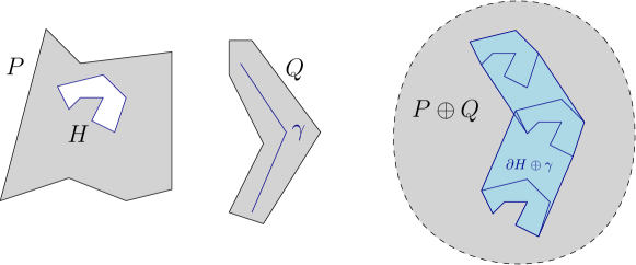
Figure 2: A small hole $H$ is irrelevant for the computation of $P\oplus Q$ as adding $\partial H$ and $\gamma\subset Q$ fills up any potential hole in $P\oplus Q$ related to $H$.

Definition 1.

A hole $H$ of polygon $P$ leaves a trace in $P\oplus Q$, if there exists a point $r=p+q\in\partial(P\oplus Q)$, such that $p\in\partial H$ and $q\in\partial Q$. We say that $r$ is a trace of $H$. Conversely, we say that a hole $H$ is irrelevant for the computation of $P\oplus Q$ if it does not leave a trace at all.

Lemma 1.

If $H$ leaves a trace in $P\oplus Q$ at a point $r$, then $r$ is on the boundary of a hole $\tilde{H}$ in $P\oplus Q$.

Proof.

Consider the point $r=p+q$, which is on the boundary of $P\oplus Q$, such that $p\in\partial H$ and $q\in\partial Q$. Since the polygons are closed, for every neighborhood of $r$ there exists a point $r^{\prime}\not\in P\oplus Q$, see Figure 3. Consequently, its corresponding point $p^{\prime}=r^{\prime}-q$, which is in the neighborhood of $p$ must be in $H$. Thus, $r^{\prime}$ must be enclosed by $\partial H\oplus q$, implying that $r^{\prime}$ is inside a hole of $P\oplus Q$. ∎

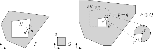
Figure 3: Hole $H$ leaves a trace in $P\oplus Q$ at point $r$, which must be on the boundary of some hole $\tilde{H}$ in $P\oplus Q$; see Lemma 1.

Lemma 2.

Let $\tilde{H}$ be a hole in $P\oplus Q$ that contains a point $r=p+q\in\partial\tilde{H}$, such that $p\in\partial H$ and $q\in\partial Q$; that is, $r$ is a trace of $H$. Then $\forall z\in\tilde{H}$ and $\forall y\in Q$, it must hold that $z\in H\oplus y$. In other words, $\tilde{H}\subseteq\bigcap_{\forall y\in Q}H\oplus y$.

Proof.

As in Lemma 1, there is a point $r^{\prime}$ in the neighborhood of $r$, which is enclosed by $\partial H\oplus q$. Furthermore, there exists a continuous path from $r^{\prime}\in\tilde{H}$ to any $z\in\tilde{H}$, which means that every $z\in\tilde{H}$ is also enclosed by $\partial H\oplus q$, or in other words: $z\in H\oplus q$.

Now, assume for contradiction that there is a point $y_{0}\in Q$, for which $z$ is not in $H\oplus y_{0}$. Consider the continuous path $\gamma$ that connects $q$ and $y_{0}$ within $Q$. Observe that $z\in H\oplus q$ and $z\notin H\oplus y_{0}$ are equivalent to $z-q\in H$ and $z-y_{0}\notin H$, respectively. This means that $z-y_{0}$ is either in the unbounded face, or in some other hole in $P$. Now observe that the path $z\oplus(-\gamma)$ connects $z-q$ and $z-y_{0}$. Thus, since $\gamma$ is continuous, there must be a point $y_{0}^{\prime}\in\gamma\subset Q$, for which $z-y_{0}^{\prime}\in P$. Hence, $z\in P\oplus y_{0}^{\prime}$, which implies $z\in P\oplus Q$—a contradiction. ∎

Corollary 1.

Let $\tilde{H}$ be a hole in $P\oplus Q$ with $r\in\partial\tilde{H}$ being a trace of $H$. Then $\forall s\in\partial\tilde{H}$ it holds that $s$ is a trace of $H$.

Proof.

By Lemma 2 $\tilde{H}\subseteq\bigcap_{\forall y\in Q}H\oplus y$ ∎

Theorem 1.

Let $H$ be a closed hole in polygon $P$. $H$ is irrelevant for the computation of $P\oplus Q$ iff there is a path contained in polygon $Q$ that does not fit under any translation in $-H$.

Proof.

We first show that $H$ is irrelevant for the computation of $P\oplus Q$ if there is a path $\gamma\subset Q$ that does not fit under any translation in $-H$. Assume for contradiction that $H$ leaves a trace in $P\oplus Q$; that is, there is an $r=p+q\in\partial(P\oplus Q)$, such that $p\in\partial H$ and $q\in\partial Q$. By Lemma 1, the point $r$ is on the boundary of a hole $\tilde{H}$ in $P\oplus Q$. By Lemma 2, for any point $x\in\tilde{H}$ it must hold that $x\in H\oplus y$ $\forall y\in Q$. Specifically, it must hold $\forall y\in\gamma\subset Q$. This is equivalent to $y\in(x\oplus-H)$ for all $y\in\gamma$, stating that $\gamma$ fits into $-H$ under some translation—a contradiction.

Conversely, if there is no path that does not fit into $-H$ then all paths contained in $Q$ fit in $-H$. Thus, also $Q$ itself fits in $-H$ under some translation $x$ with $x\oplus Q\subseteq-H$. In this case $x+q\in-H$ for all $q\in Q$, which is equivalent to $-x\in H\oplus q$ for all $q\in Q$. This implies that $-x\notin P\oplus Q$, whereas $-x\in(P\cup H)\oplus Q$, that is, H is relevant for $P\oplus Q$. ∎

Corollary 2.

If the closed axis-aligned bounding box $B_{Q}$ of $Q$ does not fit under any translation in the open axis-aligned bounding box $\mathring{B}_{H}$ of a hole $H$ in $P$, then $H$ does not have a trace in $P\oplus Q$.

Proof.

W. l. o. g. assume that $B_{Q}$ does not fit into $\mathring{B}_{H}$ with respect to the $x$-direction. Consider the two extreme points on $\partial Q$ in that direction and connect them by a closed path $\gamma$, which obviously does not fit into $-H$, as it does not fit into $\mathring{B}_{H}$. ∎

Theorem 2.

Let $P$ and $Q$ be two polygons with holes and let $P^{\prime}$ and $Q^{\prime}$ be their filtered versions, that is, with holes filled up according to Corollary 2 with $P\oplus Q=P^{\prime}\oplus Q^{\prime}$. Then, at least $P^{\prime}$ or $Q^{\prime}$ is a simple polygon.

Proof.

Note that if $B_{Q}$ does not fit in the open axis-aligned bounding box $\mathring{B}_{P}$ of $P$, it cannot fit in the bounding box of any hole in $P$, implying that all holes of $P$ can be ignored. Since for any two bounding boxes either $B_{Q}\not\subset\mathring{B}_{P}$ or $B_{P}\not\subset\mathring{B}_{Q}$ holds, we need to consider the holes of at most one polygon. ∎

Consequently, we can remove all holes whose bounding boxes are, in $x$- or $y$-direction, smaller than, or as large as, the bounding box of the other polygon, as an initial phase of all methods. With fewer holes, convex decomposition results in fewer pieces. Moreover, when all holes of a polygon become irrelevant, one can choose a decomposition method that handles only simple polygons instead of a decomposition method that handles polygons with holes, which is typically more costly. As for the convolution approach, the intermediate arrangements become smaller, speeding up the algorithm.

3 Implementation

The software has been developed as part of the 2D Minkowski Sums package of Cgal [26], and it uses other components of Cgal [23]. As such, it is written in C++ and rigorously adheres to the generic-programming paradigm the EGC paradigms. In the following we provide some details about each one of the new implementations.

3.1 Reduced Convolution

We compute the reduced convolution set of segments filtering out features that cannot possibly contribute to the boundary of the Minkowski sum (see Section 1.1) and in particular complete holes (see Section 2). Then, we construct the arrangement induced by the reduced convolution set. Finally, we traverse the arrangement and extract the boundary of the Minkowski sum. We apply two different filters to identify valid holes in the Minkowski sum: (i) We ignore any face in the arrangement the outer boundary of which forms a cycle that is not properly oriented, as suggested in [2]. (ii) We ignore any face $f$, such that $(-P\oplus x)$ and $Q$ collide, where $x\in f$ is a sampled point inside $f$, as suggested in [14]. We use axis-aligned bounding box trees to expedite the collision tests. After applying these two filters, only segments that constitute the Minkowski sum boundary remain.

3.2 Decomposition

Vertical decomposition [12] (a.k.a. trapezoidal decomposition) and triangulation [3] have been extensively used ever since they have been independently introduced a long time ago. We provide a brief overview of these two structures for completeness and explain how they are used in our implementations.

(a)

(b)

(c)

Figure 4: Convex decomposition. LABEL:sub@fig:decomp:polygon A polygon with holes. LABEL:sub@fig:decomp:vd Vertical decomposition of the polygon in LABEL:sub@fig:decomp:polygon. LABEL:sub@fig:decomp:tri Triangulation of the polygon in LABEL:sub@fig:decomp:polygon.

Vertical decomposition for a planar subdivisions is the partition of the (already subdivided) plane into a finite collection of pseudo trapezoids. Each pseudo trapezoid is either a trapezoid that has vertical sides, or a triangle (which is a degenerate trapezoid). Given a polygon with holes, we obtain the decomposition as follows: At every vertex of the polygon, we extend a ray upward if it does not escape the polygon, until either another vertex or an edge is hit. Similarly, we extend a ray downward; see Figure 4b. In our implementation we exploit the vertical decomposition functionality provided by the Cgal package 2D Arrangements [27].

A Delaunay triangulation for a set of points in a plane is the partition of the plane into triangles, such that no point in the input is inside the circumcircle of any triangle in the triangulation. A constrained Delaunay triangulation is a generalization of the Delaunay triangulation that forces certain required segments into the triangulation. Given a polygon with holes we obtain the constrained Delaunay triangulation confined to the given polygon and provide the polygon edges as constraints; see Figure 4c. In our implementation, we use the 2D Triangulations [28] Cgal package.

4 Experiments

We have conducted our experiments on families of randomly generated simple and general polygons from AGPLib [4]; examples are depicted in Figure 5a and 5b, respectively. All experiments were run on an Intel Core 2 Duo P9600 CPU clocked at 2.53 GHz with 4 GB of RAM. For each instance size the diagrams in the figures show an average over 10 runs on different input. Every run was allowed 20 minutes of CPU time and aborted when it did not finish within this limit.

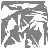
(a)

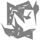
(b)

Figure 5: Randomly generated polygons: (a) simple polygon with 200 vertices, and (b) general with 200 vertices and 20 holes.

First, we compared the running time of the implementations of all methods for simple polygons available in Cgal (for details, see [8, Section 9.1.2]), the new implementations, and Behar and Lien’s implementation; see Figure 7a. The reduced convolution method consumed about ten times less time than the full convolution method for large instances, whereas the decomposition methods were the fastest for instances larger than 150 vertices. inline]why?

Secondly, we compared the running time of the implementations of the three new methods (i.e., the reduced convolution (RC), the triangular decomposition (TD), and the vertical decomposition (VD)) and Behar and Lien’s implementation on instances of general polygons with $n$ vertices and $n$/10 holes; see Figure 7b. For each pair of polygons, one was scaled down by a factor of 1000, to avoid the effect of the hole filter in this experiment. For all executions, the reduced convolution method consumed significantly less time than the two decomposition methods. Behar and Lien’s implementation generally performs worse than our reduced convolution method.

In order to demonstrate the effect of the hole filter, we compared the running time of the implementations above fed with a square of varying size (see the horizontal axis in Figure 7c and  7d) and with randomly generated polygons having 2000 vertices and 200 holes. Without the hole filter the running time of the reduced convolution method increases as the square grows due to an increase of the complexity of the intermediate arrangement. Behar and Lien’s implementation exhibited constant running time, as it performs pairwise intersection testing. When applying the hole filter to our methods, the reduced convolution method consumed less time than all other methods. The two diagrams clearly show the impact of filtering holes.

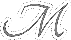
(a)

(b)

Figure 6: Letters from the font Tangerine used for the real-world benchmark, displayed with their offset versions. (a) Lowest-resolution “M” with 75 vertices (b) Highest-resolution “A” with 8319 vertices.

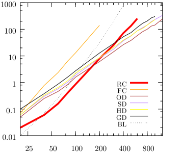
(a)

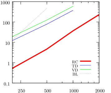
(b)

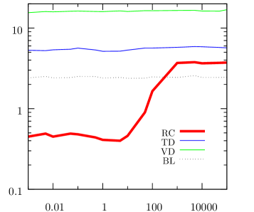
(c)

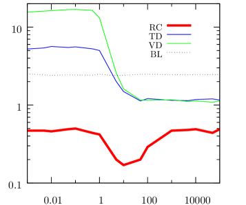
(d)

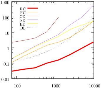
(e)

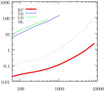
(f)

Figure 7: Time in seconds for different methods to compute Minkowski sums for two polygons. $x$-axis: #vertices of each input polygon, if not stated otherwise. Legend: (RC) reduced convolution; (FC) full convolution; (TD) constrained triangulation decomposition; (VD) vertical decomposition; (SD) small-side angle-bisector decomposition; (OD) optimal convex decomposition; (HD) Hertel-Mehlhorn decomposition; (GD) Greene decomposition; (BL) Behar and Lien’s reduced convolution.

Note that the polygons used for the benchmarks above do not represent a real-world case. Instead, the complex shapes rather constitute a worst-case, as most segments intersections are inside the Minkowski sum anyway. For a more realistic scenario, consider a text, which we want to offset (for example, for printing stickers). In Figure 7e, we show the running times of the methods available for simple polygons when calculating the Minkowski sum of a letter “M” (Figure 6) with a varying amount of vertices and a circle with 128 vertices. In Figure 7f, we show the running times of the methods available for general polygons when calculating the Minkowski sum of a letter “A” and the same circle. For both letters, our implementation of the reduced convolution is at least 5 times faster than all other methods.

5 Conclusion

All new implementations introduced in this work will be available as part of the next public release of CGAL, which now also supports polygons with holes. The decomposition approaches that handle only simple polygons outperform the new reduced convolution method (which, naturally handles also simple polygons) for instances of random simple polygons with more than 150 vertices. However, these rather chaotic polygons somewhat constitute the worst case scenario for the reduced convolution method. In all other scenarios, the reduced convolution method with hole filter outperforms all other methods by a factor of at least 5. Consequently, this is the new default method of CGAL to compute Minkowski sums for simple polygons as well as polygons with holes.

References

- [1] P. K. Agarwal, E. Flato, and D. Halperin. Polygon decomposition for efficient construction of Minkowski sums. Comput. Geom. Theory Appl., 21:39–61, 2002.
- [2] E. Behar and J.-M. Lien. Fast and robust 2D Minkowski sum using reduced convolution. In Proc. IEEE Conf. on Intelligent Robots and Systems, 2011.
- [3] M. Bern. Triangulations and mesh generation. In J. E. Goodman and J. O’Rourke, editors, Handb. Disc. Comput. Geom., chapter 25, pp. 529–582. Chapman & Hall/CRC, Boca Raton, FL, 2nd edition, 2004.
- [4] M. C. Couto, P. J. de Rezende, and C. C. de Souza. Instances for the Art Gallery Problem, 2009. http://www.ic.unicamp.br/cid/Problem-instances/Art-Gallery.
- [5] G. Elber and M.-S. Kim. Offsets, sweeps, and Minkowski sums. Comput. Aided Design, 31(3):163, 1999.
- [6] E. Fogel and D. Halperin. Exact and efficient construction of Minkowski sums of convex polyhedra with applications. In Proc. 8th Workshop Alg. Eng. Experiments, pp. 3–15, 2006.
- [7] E. Fogel and D. Halperin. Polyhedral assembly partitioning with infinite translations or the importance of being exact. IEEE Trans. on Automation Sci. and Eng., 10:227–241, 2013.
- [8] E. Fogel, D. Halperin, and R. Wein. Cgal Arrangements and Their Applications, A Step by Step Guide. Springer, Berlin Heidelberg, Germany, 2012.
- [9] P. K. Ghosh. A unified computational framework for Minkowski operations. Comput. & Graphics, 17(4):357–378, 1993.
- [10] L. J. Guibas, L. Ramshaw, and J. Stolfi. A kinetic framework for computational geometry. In Proc. 24th Annu. IEEE Symp. Found. Comput. Sci., pp. 100–111, 1983.
- [11] P. Hachenberger. Exact Minkowksi sums of polyhedra and exact and efficient decomposition of polyhedra into convex pieces. Algorithmica, 55(2):329–345, 2009.
- [12] D. Halperin. Arrangements. In J. E. Goodman and J. O’Rourke, editors, Handb. Disc. Comput. Geom., chapter 24, pp. 529–562. Chapman & Hall/CRC, Boca Raton, FL, 2nd edition, 2004.
- [13] E. E. Hartquist, J. Menon, K. Suresh, H. B. Voelcker, and J. Zagajac. A computing strategy for applications involving offsets, sweeps, and Minkowski operations. Comput. Aided Design, 31:175–183, 1999.
- [14] A. Kaul, M. O’Connor, and V. Srinivasan. Computing Minkowski sums of regular polygons. In Proc. 3rd Canadian Conf. on Comput. Geom., pp. 74–77, 1991.
- [15] L. E. Kavraki. Computation of configuration-space obstacles using the fast fourier transform. In Proc. IEEE Int. Conf. on Robotics & Automation, pp. 255–261, 1993.
- [16] J.-C. Latombe. Robot Motion Planning. Kluwer Academic Publishers, Norwell, Massachusetts, 1991.
- [17] W. Li and S. McMains. A GPU-based voxelization approach to 3D Minkowski sum computation. In Proc. 2010 ACM Symp. Solid Phys. Model., pp. 31–40. ACM Press, 2010.
- [18] J.-M. Lien. A simple method for computing Minkowski sum boundary in 3D using collision detection. In H. Choset, M. Morales, and T. D. Murphey, editors, Alg. Foundations of Robotics VIII, volume 57 of Springer Tracts in Advanced Robotics, pp. 401–415. Springer, 2009.
- [19] M. C. Lin and D. Manocha. Collision and proximity queries. In J. E. Goodman and J. O’Rourke, editors, Handb. Disc. Comput. Geom., chapter 35, pp. 787–807. Chapman & Hall/CRC, Boca Raton, FL, 2nd edition, 2004.
- [20] T. Lozano-Pérez. Spatial planning: A configuration space approach. IEEE Trans. on Comput., C-32:108–120, 1983.
- [21] V. Milenkovic and E. Sacks. A monotonic convolution for Minkowski sums. Int. J. of Comput. Geom. Appl., 17(4):383–396, 2007.
- [22] G. Ramkumar. Tracings and Their Convolutions: Theory and Application. Phd thesis, Stanford, California, 1998.
- [23] The Cgal Project. Cgal User and Reference Manual. Cgal Editorial Board, 4.6 edition, 2015. http://doc.cgal.org/latest/Manual/index.html.
- [24] G. Varadhan and D. Manocha. Accurate Minkowski sum approximation of polyhedral models. Graphical Models, 68(4):343–355, 2006.
- [25] R. Wein. Exact and efficient construction of planar Minkowski sums using the convolution method. In Proc. 14th Annu. Eur. Symp. Alg., pp. 829–840, 2006.
- [26] R. Wein. 2D Minkowski sums. In Cgal User and Reference Manual. Cgal Editorial Board, 4.6 edition, 2015. http://doc.cgal.org/latest/Manual/packages.html#Pkg{Minkowski}Sum2Summary.
- [27] R. Wein, E. Berberich, E. Fogel, D. Halperin, M. Hemmer, O. Salzman, and B. Zukerman. 2D arrangements. In Cgal User and Reference Manual. Cgal Editorial Board, 4.6 edition, 2015. http://doc.cgal.org/latest/Manual/packages.html#PkgArrangement2Summary.
- [28] M. Yvinec. 2D triangulations. In Cgal User and Reference Manual. Cgal Editorial Board, 4.6 edition, 2015. http://doc.cgal.org/latest/Manual/packages.html#PkgTriangulation2Summary.