Bosonic Kondo-Hubbard model

Abstract

We study, using quantum Monte-Carlo simulations, the bosonic Kondo-Hubbard model in a two dimensional square lattice. We explore the phase diagram and analyse the mobility of particles and magnetic properties. At unit filling, the transition from a paramagnetic Mott insulator to a ferromagnetic superfluid appears continuous, contrary to what was predicted with mean field. For double occupation per site, both the Mott insulating and superfluid phases are ferromagnetic and the transition is still continuous. Multiband tight binding Hamiltonians can be realized in optical lattice experiments, which offer not only the possibility of tuning the different energy scales over wide ranges, but also the option of loading the system with either fermionic or bosonic atoms.

I Introduction

In condensed matter systems, the interaction between mobile particles and fixed magnetic impurities, known as Kondo physics, has been a very important topic for the last 50 years. From the original explanation of the resistance minimum in metals with magnetic impurities by Kondo, to the investigation of the properties of heavy fermion materials, the interaction between particles and localized spins has revealed a variety of interesting physical phenomena hewson93 ; tsunetsugu97 . Indeed, the competition between magnetic ordering and singlet formation in Kondo and related materials has offered some of the most fundamental examples of quantum phase transitions wang06 , and investigations of the effects of interplay of the distinct spin and particle contributions to the susceptibility, and of dilutionassaad02 ; seo14 , are at the frontier of the investigation of many materials, including the ‘115’ heavy fermion family shirer12 ; seo14

In addition to these solid state systems, with the recent experimental advances in ultracold atomic physics, it is now possible to build systems of atoms on optical lattices with atoms occupying different bands hemmerich11 ; mueller07 ; clement09 . This opens the possibility to use the atoms located in the lowest band as localized particles, magnetic centres, which will interact with mobile particles located in higher energy bands. Such systems would be analogues of Kondo problems but with the possibility to use bosonic particles instead of fermionic ones, systems that have not been extensively studied and are not available in condensed matter physics.

We will study here a system similar to the Kondo-Hubbard lattice problem tsunetsugu97 ; feldbacher02 ; yanagisawa95 ; fazekas97 with interacting spin 1/2 bosons instead of fermions. Mobile bosons are free to move on the lattice and interact repulsively on site. In addition, there is an antiferromagnetic (AF) coupling to an ensemble of spin 1/2 magnetic centres, one for each site of the lattice. This model was introduced by Duan duan04 to describe the following system: the localized bosonic species (‘spins’) are atoms in the lowest band of an optical lattice with a potential barrier which prohibits tunneling. The mobile species occupy an upper band, to which they have been excited through the applicaton of periodic Raman pulses, which allows tunneling. This model was studied in detail with different analytical techniques by Foss-Feig and Rey fossfeig11 . In fossfeig11 , exact results were derived for the small and large interaction limits and the intermediate regime was studied using mean-field theory, for different densities of particles. For one mobile particle per site, they observed a first order transition between a Mott insulator (MI) phase and a superfluid (SF) phase as the interaction is lowered. In the Mott phase, there are singlets of bosons and spin and no long range magnetic order whereas the SF phase shows long range ferromagnetic (FM) order for the bosons and the spins. For two or more particles per site, the Mott phase is already ferromagnetic and the transition to the ferromagnetic superfluid state is continuous.

In this paper, we will use exact quantum Monte Carlo simulations to study this bosonic Kondo-Hubbard model duan04 and determine exactly the phase diagram and magnetic properties of the system at zero and finite temperatures $T$ and compare with results previously obtained with mean-field approximations duan04 ; fossfeig11 . In Sec. II, we introduce the model, the numerical technique we used and the quantities we will measure to characterize the phases. In Sec. III, we study the transport properties and Green functions of the system to draw its phase diagram at $T=0$. In Sec. IV we analyse in more detail the nature of the quantum phase transitions. Sec. V is devoted to a careful analysis of the magnetic properties in the ground state and Sec. VI presents the evolution of the phases observed at $T=0$ as the temperature is increased.

II Bosonic Kondo-Hubbard model

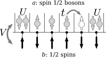
Figure 1: Schematic representation of the model. Spin-$1/2$ bosons (upper layer $a$) are moving through the lattice with hopping $t$ and are subject to on-site repulsion $U$. They interact antiferromagnetically with strength $V$ with the lower spin layer $b$. The lattice represented here is a 1D chain; the studied system is a 2D square lattice.

The system we consider includes two types of objects that are coupled antiferromagnetically (AF): spin-$1/2$ bosons which hop on a 2D square lattice and, on every site, a fixed spin-$1/2$ magnetic impurity. In the following, we will denote the bosons as particles of type $a$ and the fixed spins as particles of type $b$. An easy way to visualize this system is to use two layers, $a$ and $b$, one filled with bosons, the other with spins (Fig. 1). The Hamiltonian reads

$${\cal H} = -t\sum_{\langle i,j\rangle,\sigma}\left(a^{\dagger}_{i,\sigma}a^{\phantom{\dagger}}_{j,\sigma}+{\rm h.c.}\right)$$ (1)

$$+ \frac{U}{2}\sum_{i}n_{a,i}\left(n_{a,i}-1\right)$$ (2)

$$+ V\sum_{i}{\bf S}_{a,i}\cdot{\bf S}_{b,i}$$ (3)

The operators $a^{\dagger}_{i,\sigma}$ and $a_{i,\sigma}$ create or destroy an $a$-type boson of spin $\sigma$ on site $i$. The system is a 2D square lattice with $L^{2}$ sites where $L$ is the length of the lattice. There is always one $b$ spin per site and we will vary the number $N_{a}$ of $a$ bosons. The Hamiltonian includes a hopping term (Eq. 1) and an on site repulsion (Eq. 2) for the $a$ bosons. $n_{a,i}=\sum_{\sigma}n_{a,i,\sigma}=\sum_{\sigma}a^{\dagger}_{i,\sigma}a^{\phantom{\dagger}}_{i,\sigma}$ is the total number of bosons on site $i$. The hopping parameter $t$ sets the energy scale and the on-site repulsion energy is $U$.

The last term (Eq. 3) of the Hamiltonian is an antiferromagnetic coupling between the boson magnetic moment and the fixed $b$ spins. ${\bf S}_{a,i}=(S^{x}_{a,i},S^{y}_{a,i},S^{z}_{a,i})$ gives the spin of the bosons and its components are given by

$$S^{\alpha}_{a,i}=\sum_{\sigma,\sigma^{\prime}}a^{\dagger}_{i,\sigma}S^{\alpha}_{\sigma,\sigma^{\prime}}a^{\phantom{\dagger}}_{i,\sigma^{\prime}}$$ (4)

where the $S^{\alpha}_{\sigma,\sigma^{\prime}}$ are the three standard spin 1/2 matrices. The $b$ spins are also described by these matrices ${\bf S}_{b,i}=(S^{x}_{b,i},S^{y}_{b,i},S^{z}_{b,i})$. To specify a state of the system one should give the state $S^{z}_{b,i}=\pm 1/2$ of each $b$ spin and the number $n_{a,i,\sigma}$ of up or down $a$ bosons present on each site $i$. The conventional quantum number $s$ will be used when discussing the possible eigenvalues of angular momentum ${\bf S}^{2}=s(s+1)$.

The last term of the Hamiltonian is the Kondo interaction, here in the form used in the Kondo insulators where the moving particles interact with a network of magnetic moments. This is different from the original Kondo problem where the moving particles are coupled to a small number of magnetic “impurities” distributed randomly hewson93 and more similar to the “Kondo lattice” fazekas91 . Other differences with the original Kondo problem are that our moving particles are not free but interacting with each other and, of course, they are bosons and not fermions. Studying an equivalent spin 1 model would be interesting but is more demanding numerically. The spin 1/2 model allows us to compare with the results from fossfeig11 ; duan04 , which also propose an experimental realization of the model. Furthermore the qualitative physics should not be different with a spin 1 model.

To study this system, we used the quantum Monte Carlo SGF algorithm rousseau08 ; rousseau08-2 that allows exact calculations of physical observables at finite temperature on clusters of finite size (up to $L=14$). We are especially interested in one and two-body Green functions that are possible to calculate with the SGF algorithm. To extract the properties of the ground state, we used large inverse temperatures $\beta=1/kT$, up to $\beta t=25$.

We studied the one-body Green functions for the bosons $G_{a,\sigma}(R)$,

$$G_{a,{\sigma}}(R)=\frac{1}{2L^{2}}\sum_{i}\langle a^{\dagger}_{i,\sigma}a^{\phantom{\dagger}}_{i+R,\sigma}+a^{\dagger}_{i+R,\sigma}a^{\phantom{\dagger}}_{i,\sigma}\rangle.$$ (5)

The condensed fraction $\rho(k=0)$ is the Fourier transform at $k=0$, $\rho(k=0)=\sum_{R,\sigma}G_{a,{\sigma}}(R)/L^{2}$. The superfluid density $\rho_{s}$ can be measured using the standard relation with fluctuations of the winding number $\rho_{s}=\langle W^{2}\rangle/4t\beta$ as the total number of bosons is conserved ceperley89 .

We also studied anticorrelated two-body Green functions which describe exchange of particles or spins at long distances, which then correspond to opposite, anticorrelated movements. They are generally important for multispecies Hamiltonians with repulsive interactions where exchanges are the dominant effects in the strongly interacting regimes kuklov03 . In this case, they are conveniently expressed in terms of spin degrees of freedom

$$G_{aa}(R) = \frac{1}{2L^{2}}\sum_{i}\langle a^{\dagger}_{i,\uparrow}a^{\phantom{\dagger}}_{i,\downarrow}a^{\phantom{\dagger}}_{i+R,\uparrow}a^{\dagger}_{i+R,\downarrow}+{\rm h.c.}\rangle$$ (6)

$$= \frac{1}{2L^{2}}\sum_{i}\langle S^{+}_{a,i}S^{-}_{a,i+R}+{\rm h.c.}\rangle$$

$$G_{bb}(R) = \frac{1}{2L^{2}}\sum_{i}\langle S^{+}_{b,i}S^{-}_{b,i+R}+{\rm h.c.}\rangle$$ (7)

$$G_{ab}(R) = \frac{1}{2L^{2}}\sum_{i}\langle a^{\dagger}_{i,\uparrow}a^{\phantom{\dagger}}_{i,\downarrow}S^{-}_{b,i+R}+{\rm h.c.}\rangle$$ (8)

$$= \frac{1}{2L^{2}}\sum_{i}\langle S^{+}_{a,i}S^{-}_{b,i+R}+{\rm h.c.}\rangle$$

As $(S^{+}_{i}S^{-}_{i+R}+S^{-}_{i}S^{+}_{i+R})=2(S^{x}_{i}S^{x}_{i+R}+S^{y}_{i}S^{y}_{i+R})$, they correspond to the spin correlations in the $x-y$ plane.

Adding the spin-spin correlations along the $z$ axis (which are diagonal quantities) to the correlations in the $xy$ plane that were obtained through Green functions, we obtain the complete spin-spin correlations. For example,

$$S_{aa}(R)=\frac{1}{L^{2}}\sum_{i}\langle{\bf S}_{a,i}\cdot{\bf S}_{a,i+R}\rangle.$$ (9)

Similar definitions hold for correlations $S_{bb}(R)$ between the $b$ spins and for correlations $S_{ab}(R)$ between bosons and spins. We will denote by ${\bf S}_{\rm tot}=\sum_{i}({\bf S}_{a,i}+{\bf S}_{b,i})$ the total spin, or total magnetization, of the system, which is expressed as a sum of spin correlations functions

$$S^{2}_{\rm tot}=\sum_{R}\left[S_{aa}(R)+2S_{ab}(R)+S_{bb}(R)\right]$$

III Phase Diagram

We first show the phase diagram in the $(t/U,\mu/U)$ plane at $T=0$ for a fixed value of $V/U=0.05$ (Fig. 2). For small values of $V/U$, some of the transitions in the system are predicted to be first order fossfeig11 . At $T=0$, using a canonical simulation, the chemical potential is given by the energy difference $\mu(N_{a})=E(N_{a}+1)-E(N_{a})$ where $N_{a}$ is the number of bosons. This allows to draw the boundaries of the $n$th Mott lobe with $n$ bosons of type $a$ per site by measuring the energy of the system with $N_{a}=nL^{2},nL^{2}+1$, and $nL^{2}-1$ particles. In the $t/U=0$ limit, an analytical calculation yields fossfeig11 $\mu_{0\rightarrow 1}=-3V/4$, $\mu_{1\rightarrow 2}=U-V/4$, $\mu_{2\rightarrow 3}=2U-V/4$, where $\mu_{n\rightarrow n+1}$ is the value at which the density changes from $n$ to $n+1$. In Fig. 2, we exhibit the $\rho=1$ and $\rho=2$ insulating Mott lobes. Outside of these Mott lobes, the system is superfluid and Bose condensed, as we will show below. The first Mott lobe is paramagnetic and the rest of the phase diagram has ferromagnetic correlations of the bosons.

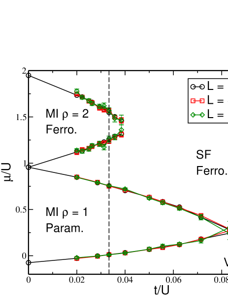
Figure 2: Phase diagram for several system sizes $L$. The insulating phase at $\rho=1$ is paramagnetic while the other phases are ferromagnetic. The dashed line indicates the cut in Figure 10.

Compared to other studies of spin-$1/2$ bosons or mixtures of particles deforges11 , the Mott lobes are larger. As expected, the presence of the Kondo interaction favours insulating behaviour: The tip of the $\rho=1$ Mott lobe is located around $t/U\simeq 0.08$ for $V/U=0.05$ whereas it is located around $t/U\simeq 0.06$ for $V=0$. As $V/U$ is increased up to 0.25, the tip shifts further to $t/U\simeq 0.10$ (see Fig. 12). This robustness is not surprising since, for $\rho=1$, the Mott gap is equal to $U+V/2$ fossfeig11 in the $t=0$ limit.

Analysing the Green functions at $\rho=1$, we observe that they all decrease rapidly to zero with distance in the Mott phase and there is no phase coherence (Fig.3 (a)). This is expected for the one-body Green functions but is also the case for the anticorrelated Green functions. In the $t=0$ limit, to minimize the AF energy between the spins and bosons, the magnetic moment of the boson forms a singlet with the spin located at the same site. As these singlets are formed, there is a unique Mott state in the $t=0$ limit and there is no possibility to exchange bosons of different spins kuklov03 . This behaviour is probably maintained throughout the $\rho=1$ Mott lobe, even at $t\neq 0$. This is verified by the value of $G_{ab}(0)\simeq-0.5$ which shows the on-site antiferromagnetic correlation of the magnetic moments and will be confirmed below by direct measurements of the magnetic correlations.

In the superfluid phase at $\rho=1$ (Fig.3 (b)), on the other hand, all the Green functions show long range order. The long range order of the one-body Green function $G_{a,\sigma}$ shows that the system is Bose condensed. The non zero value of $G_{aa}$ shows that, in addition to the individual movement of the particles, exchange moves are important degrees of freedom for this phase. $G_{bb}$ is non zero, which shows that the spins are correlated. This correlation is mediated by the movement of the bosons as the spins are not directly linked to each other. This is confirmed by the observation that the boson-spin Green function, $G_{ab}$, is also non zero. While $G_{aa}$ and $G_{bb}$ are positive, which signals ferromagnetic behaviour, $G_{ab}$ is negative which is expected since the coupling between bosons and spins is AF. The picture that emerges from these results is that the bosons and the spins form ferromagnetic phases but that these two species are coupled in an antiferromagnetic way (Fig.4).

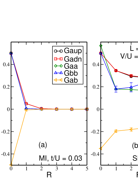
Figure 3: The one-body and the anticorrelated Green functions versus distance $R$ in the Mott insulator (a) and superfluid phase (b) for $\rho=1$. (a) all movement is suppressed as the particles form singlets. (b) movement of individual particles as well as anticorrelated exchanges are observed.

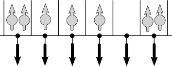
Figure 4: The magnetic order that appears in the system. While the bosons and the spins form ferromagnetic layers, these two layers are coupled antiferromagnetically.

For $\rho=2$, the Mott phase behaves differently from $\rho=1$ (Fig. 5 (a)). The individual movement of particles are still suppressed: $G_{a,\sigma}$ goes to zero with distance. However exchange movements are present and, consequently, there are couplings between the spins as is seen from the anticorrelated Green functions taking finite values at large distances. This can be understood by noting that the ground state in the $t=0$ limit is not unique fossfeig11 . This degeneracy will be lifted by a non zero hopping term and give a ground state with ferromagnetic correlations between the bosons. The magnetic order present in this phase is then similar to the one observed in the superfluid phase.

The $\rho=2$ superfluid phase (Fig. 5 (b)) shows the same qualitative behaviour as the $\rho=1$ SF phase. However the dominant behaviour in this case is the anticorrelated movements of bosons whereas they were individual movements of bosons at $\rho=1$. This is expected since, in a strongly correlated system, particles can move with a partner while individual movement is suppressed. Of course, as the density increases, the correlations become more prominent.

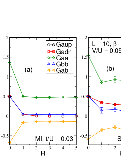
Figure 5: The one-body and the anticorrelated Green functions versus distance $R$ in the Mott insulator (a) and superfluid (b) phases for $\rho=2$. (a) Individual movement are suppressed but anticorrelated moves are possible in the Mott phase. (b) All kind of movements are present in the superfluid phase.

IV Quantum Phase transitions

We now analyse the nature of the phase transitions between the Mott and the superfluid phases by examining the behaviour of the superfluid density. In the Mott lobe $\rho_{s}=0$; as $t/U$ is increased at fixed $\rho=1$ and $V/U=0.05$, we observe a seemingly continuous transition from the MI to the SF (Fig. 6). We fit the curves near the transition with a form $\rho_{s}\propto(t/U-t/U_{c})^{\beta}$ (Fig. 6) and found $\beta\simeq 0.33$. It is however difficult to distinguish a continuous transition with a small $\beta$ coefficient (which gives a large slope close to the transition) from a discontinuous one on such finite size systems. The condensate density $\rho(k=0)$ shows a similar behaviour (Fig. 7), as expected in two dimensions in the zero temperature limit where both $\rho_{s}$ and $\rho(k=0)$ are non zero in the superfluid phase. A continuous transition is in disagreement with the MF analysis from fossfeig11 that predicts a first order, discontinuous, transition when $V/U<0.1$, which is the case here. To confirm this result, we calculated $\rho(\mu)$ in the canonical ensemble and did not find a negative compressibility region which would have been a clear sign of a discontinuous transition batrouni00 . We also observe no sign of a discontinuity at the tip of the $\rho=1$ Mott lobe, if there is one, as predicted in fossfeig11 , it is too small to discern for the system sizes accessible to us. In Fig. 8, we show the evolution of this behaviour for a given size as $t/U$ is increased. As $V/U$ becomes larger the behaviour becomes smoother and the transition still appears continuous.

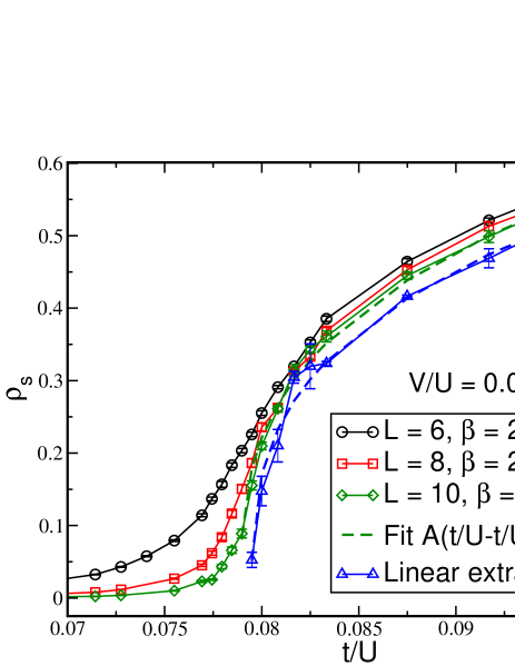
Figure 6: Superfluid density, $\rho_{s}$, versus $t/U$ in the first Mott lobe. We observe a continuous behavior for $\rho_{s}$. The blue curve with triangles represents a linear extrapolation to $L=\infty$ of the results obtained for the three sizes $L=6,\,8,\,10$. The curves for $L=10$ and the extrapolated one have been fitted with a power law behavior $\rho_{s}\propto(t/U-t/U_{c})^{\beta}$ (dashed lines). In both cases, we found $t/U_{c}\simeq 0.79$ and $\beta\simeq 0.33$.

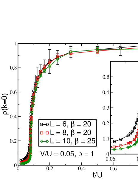
Figure 7: Condensate fraction, $\rho(k=0)$, versus $t/U$ in the first Mott lobe. The shape is very similar to figure 6, confirming the order of the transition.

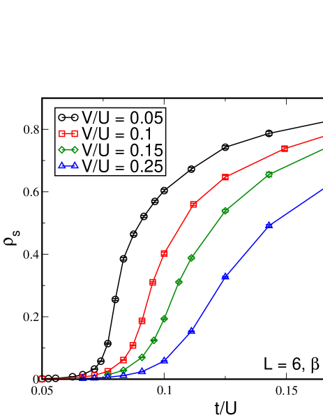
Figure 8: Superfluid density, $\rho_{s}$, versus $t/U$ in the first Mott lobe, for different ratio $V/U$. As we increase this ratio, $\rho_{s}$ becomes smoother, compared to Fig. 6 and the transition remains second order.

In Fig. 9 we show $\rho_{s}$ as a function of $t/U$ for the $\rho=2$ Mott-SF transition and do not observe a discontinuity between the two phases: the transition is continuous for all $V/U$.

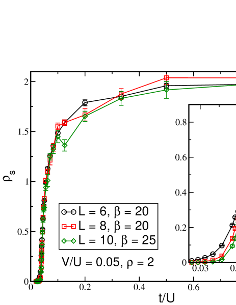
Figure 9: Superfluid density, $\rho_{s}$, versus $t/U$ in the second Mott lobe. As for the $\rho=1$ case (Fig. 6), we do not observe any discontinuity in $\rho_{s}$ and the transition is second-order.

In figure 10, we examine the dependence of $\rho$ and $\rho_{s}$ on the chemical potential $\mu$ along the dashed line in Fig. 2. We observe the conventional incompressible Mott plateaux where $d\rho/d\mu=0$. The superfluid density goes to zero continuously as these plateaux are approached, showing that the transition for the $\rho=1$ Mott is, as mentioned earlier, continuous. $\rho(\mu)$ is also continuous and has a positive slope, there is thus no sign of a phase separation close to the transition.

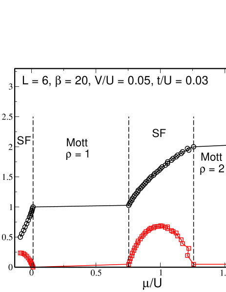
Figure 10: Cut of figure 2 for $t/U=0.03$, showing the total density, $\rho$, and the superfluid density, $\rho_{s}$, as functions of $\mu/U$. All the transitions are continuous.

V Magnetic properties

We now study in more detail the magnetic properties of the system. We plot $S_{\alpha\beta}(L/2)$ at the largest possible distance $L/2$. For a sufficiently large system this converges to the square of the magnetization of a given layer. We also study the on-site correlation to see if singlets are formed between the $a$ and $b$ layers, and the total spin of the system $S^{2}_{\rm tot}/L^{4}$.

In Fig. 11 we plot these quantities as functions of $t/U$ for $\rho=1$. We observe that in the Mott phase, the magnetic correlations are always zero. $S_{ab}(0)=-3/4$ signals the formation of a singlet. As the $a$ and $b$ particles form a singlet on each site, the absence of magnetic correlations between sites is reasonable. In the superfluid phase, on the other hand, we observe that we no longer have a singlet phase as $S_{ab}(0)$ departs from the value observed in the Mott phase. We also observe, as anticipated earlier, that ferromagnetic correlations develop between the $a$ bosons, between the $b$ spins and antiferromagnetic correlations persist between the two types of particles (corresponding to the positive values of $S_{aa}(L/2)$ and $S_{bb}(L/2)$ and the negative value of $S_{ab}(L/2)$). Deep in the superfluid, the magnetic correlations take their maximum possible value $|S_{\alpha\beta}(L/2)|\rightarrow 1/4$. It should be remarked that the correlation between the $b$ spins is mediated by the itinerant $a$ bosons, as there are no direct connections between the spins themselves. This is similar to the coupling between localized spins provided by the RKKY interaction ruderman54 ; kasuya56 ; yosida57 in fermionic systems, although it is always ferromagnetic in our case. Within error bars, we have $S_{aa}(L/2)=S_{bb}(L/2)=-S_{ab}(L/2)$ and, accordingly, the value of the total spin $S^{2}_{\rm tot}/L^{4}$ is zero. This was predicted in reference fossfeig11 in the high and low $t/U$ limits but we see here that this seems to be the case also for intermediate values. We then have very different magnetic behaviour (independent singlets in the Mott, magnetic order in the SF) with the same $S_{\rm tot}$. One should remarks that, whereas the antiferromagnetic correlations between bosons and spins are imposed by the Hamiltonian and were expected, the ferromagnetism of the bosons layer appears spontaneously. There is no term that directly favors the development of FM correlations between bosons compared to other spin textures.

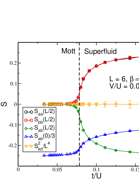
Figure 11: Magnetic correlations versus $t/U$ for $\rho=1$ and $V/U=0.05$. The dashed line marks the transition between the Mott and the superfluid phases. There is no magnetic order in the Mott phase where the $a$ and $b$ spins form singlets, as shown by the values of $S_{ab}(0)$. The superfluid phase shows the magnetic behaviour depicted in Fig.4: intra-species ferromagnetic correlations and inter-species antiferromagnetic correlations. At large $t$, the magnetic correlations tend to their maximum values.

Increasing $V$, we observe the same qualitative behaviour with some quantitative changes (Fig. 12). As mentioned earlier, the Mott-SF transition is shifted towards lower values of $U$ as the Kondo interaction is added to the repulsion between particles, which is visible in the behaviour of $\rho_{s}$. The appearance of the superfluidity and of the magnetic correlations is once again simultaneous and corresponds to the disappearance of the spin singlets. Finally we remark that the magnetic correlations tend to their maximum values but that those will be reached for much larger values of $t/U$. This is understandable as the singlets are more difficult to break at large $V$ which makes it more difficult to develop intersite correlations.

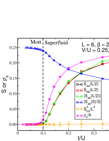
Figure 12: Magnetic correlations and $\rho_{s}$ versus $t/U$ for $\rho=1$ and $V/U=0.25$. The physical behaviour is the same as in the $V/U=0.05$ case (Fig. 11) but it is more difficult to establish the magnetic correlations with this larger value of $V$.

For $\rho=2$, deep in the Mott phase, the $a$ spins located on the same site form a total $s_{a}\approx 1$ moment, which gives $S_{aa}(0)=s_{a}(s_{a}+1)\approx 2$. This spin is then coupled antiferromagnetically to a $b$ spin which is shown by the value of $S_{ab}(0)\approx-1$, giving a total spin-$1/2$ and, consequently, two degenerate states on each site (Fig. 13). The kinetic term lifts the degeneracy between these states and we obtain the magnetic order which is observed in the SF regions and also even in the Mott lobe. Analytically fossfeig11 , it was predicted that $S_{bb}(R\neq 0)=1/36\simeq 0.0278$. For the largest value of the interaction used in our simulations $U=100t$, we observe $S_{bb}(L/2)=0.028\pm 0.001$ and, as can be seen in Fig. 13, we reached the regime where $S_{bb}(L/2)$ saturates at this non zero value.

In the superfluid phase, the system behaves very much as for $\rho=1$. $S_{aa}(0)$ and $S_{ab}(0)$ depart from their Mott phase value and increase slightly. $S_{aa}(L/2)$, $S_{bb}(L/2)$, and $S_{ab}(L/2)$ go to their extreme possible values 1, 1/4 and -1/2, respectively.

It is predicted fossfeig11 that $S^{2}_{\rm tot}=(L^{2}/2)(L^{2}/2+1)\approx L^{4}/4$ in the strong and weak coupling limits. We observe that $S^{2}_{\rm tot}/L^{4}$ always takes a value compatible with 1/4, for any value of $t/U$. As for $\rho=1$, we observe two different behaviours for the same common value of $S^{2}_{\rm tot}/L^{4}$.

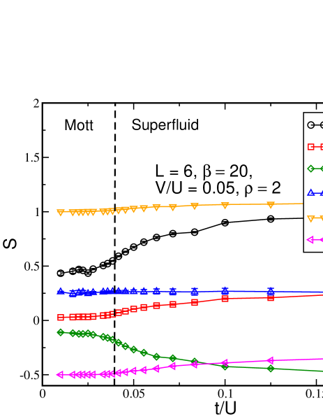
Figure 13: Magnetic correlations versus $t/U$ for $\rho=2$ and $V/U=0.05$. The dashed line marks the transition between the Mott and the superfluid phases. The same magnetic order is present in the Mott and the superfluid phases although there are two different limiting regimes with stronger (for $t/U\gg 1$) or weaker (for $t/U\ll 1$) $b$ spin correlations. The magnetic behaviour is the one sketched in Fig. 4. The total spin seems constant $S^{2}_{\rm tot}/L^{4}\simeq 1/4$.

VI Thermal effects

We analysed the behaviour of the observed phases at finite temperature. First we looked at the superfluid density to determine the extent of the superfluid phase as the temperature is increased. The thermal phase transition between the superfluid phase and the normal liquid is of the BKT type. We performed different finite size analyses to determine the critical temperature $T_{c}$ at which $\rho_{s}$ becomes zero. First we used linear extrapolations of $\rho_{s}$ as a function of $1/L$ for different values of $1/T$. Then we used Nelson and Kosterlitz’s result nelson77 $\rho_{s}(T_{c})=kT/\pi t$ to calculate the temperature $T_{c}(L)$ at which our curves intersect $kT/\pi T$ before looking at the $1/L\rightarrow 0$ extrapolation (Fig. 14). Finally we used the recently proposed method by Hsieh et al. hsieh13 . All three methods gave similar results for the system sizes accessible to us.

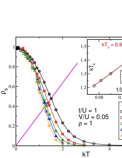
Figure 14: Superfluid density, $\rho_{s}$, versus $T$ for several sizes $L$ with $t/U=1$ and $V/U=0.05$. We calculate the intersection between the curves and $kT/\pi t$ to obtain $T_{c}(L)$. We then extrapolate linearly (see inset) the value of $T_{c}(L)$ to the large size limit to obtain the estimate of the transition temperature shown in Fig. 16.

There is no transition between the Mott phase and the normal liquid, as the Mott phase exists only at zero temperature, strictly speaking. We calculated the fluctuation of the number of particles $\kappa=\langle n_{a,i}^{2}\rangle-\langle n_{a,i}\rangle^{2}$ which exhibits a plateau at small $kT$ before increasing at higher $kT$. We identify the crossover temperature between the Mott and the liquid behaviour as the temperature where $\kappa$ departs from this low $T$ value by more than $5\%$. We checked that this definition is valid by comparing with a measure of $\rho(\mu)$ and finding the $T$ at which the Mott “plateaux” disappear in $\rho(\mu)$.

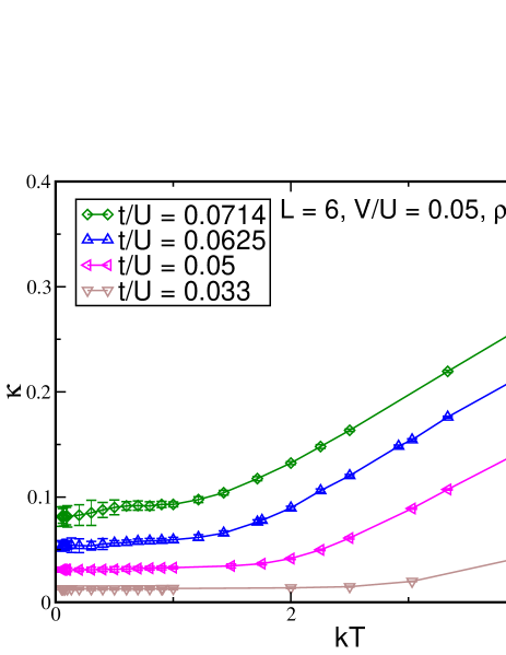
Figure 15: The local density fluctuation $\kappa=\langle n_{a,i}^{2}\rangle-\langle n_{a,i}\rangle^{2}$ versus $kT$ for different temperatures. We see that $\kappa$ is almost constant at low $kT$ in the Mott region. We defined the crossover temperature between the Mott and the liquid behaviour as the temperature for which $\kappa$ departs from its low $T$ value by more than 5%.

Putting these results together, we obtain the phase diagrams shown in Fig. 16 for $\rho=1$ and $\rho=2$. We placed at $T=0$ the point of the quantum phase transition observed in Sec. IV.

We now turn to the magnetic behaviour at finite temperature. In the Mott phase at $\rho=1$, there is no magnetic order at $T=0$ and this behaviour persists at finite temperature. In the Mott phase at $\rho=2$, the magnetic couplings that lead to a ferromagnetic phase are weak and the magnetic order disappears for low temperatures $kT\simeq 0.3$ on an $L=6$ system. As the system is well described, in the Mott phase, by a Heisenberg model, we do not expect to observe magnetic order at finite temperature in the thermodynamic limit.

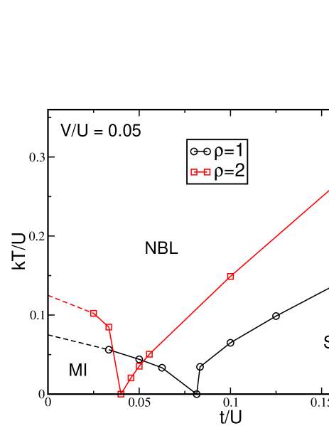
Figure 16: The phase diagrams for $\rho=1$ and $\rho=2$ as a function of $t/U$ and $kT/U$ at $V/U=0.05$. There are three different regions in each diagram: a Mott region (MI), the normal Bose liquid (NBL) and the superfluid region (SF). The SF-NBL limit is a BKT transition. The MI-NBL limit is a crossover between weakly and highly compressible regimes.

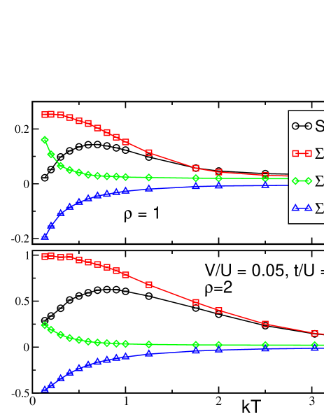
Figure 17: Magnetisation of the whole system ($S_{\rm tot}$) and sums over all distances of boson-boson ($S_{aa}$), spin-spin ($S_{bb}$) and boson-spin $(S_{ab}$) magnetic correlations for $\rho=1$ in the superfluid phase. The total magnetisation $S_{\rm tot}$ is zero at $T=0$ but rises when $T$ is increased. As the bosons decouple from the spin, when $kT>V$, and no longer form singlets with those, they develop ferromagnetic correlations. Top panel: $\rho=1$, bottom panel: $\rho=2$.

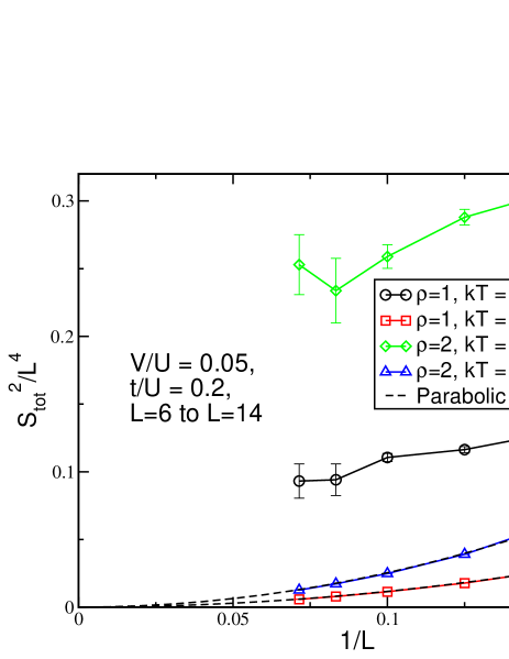
Figure 18: Extrapolation of the magnetization as a function of the size. At high temperature ($kT=4.55$) the magnetization extrapolates to zero. At the temperatures where we observed the peaks of the moment in Fig. 17 the magnetization does not seem to extrapolate to zero. The data for $\rho=2,kT=0.9$ have been divided by 2 for better visibility.

The behaviour in the superfluid regime is much more interesting. What we observe is that the magnetic ordering is reinforced when we increase the temperature from $T=0$. We find that the total magnetisation $S_{\rm tot}$ increases before decreasing again and reaching zero in the high temperature regime (see Fig. 17). The increase of the total magnetisation is due to a strong decrease of the boson-spin $S_{ab}$ correlations. This is easily understood as the coupling $V$ between bosons and spins takes a small value ($V/U=0.05$). Thermal excitations break the correlations between spins and bosons. The AF correlation between those two species disappears and the spins are then disordered as the bosons no longer mediate an intersite coupling. As the bosons become independent of the spins, they form a FM superfluid with a larger total magnetisation. Once again, the mechanism for this FM ordering is not clear but it is obviously mediated by the hopping of bosons, the only effect that can couple distant particles in this system. As the hopping $t$ is larger than $V$ these remaining FM correlations disappear only at larger temperatures. For example, for $\rho=1$ (Fig. 17) the AF correlations $S_{ab}$ and the spin-spin correlations $S_{bb}$ have almost disappeared for $kT=1$ whereas the FM correlations $S_{aa}$ become negligible only for $kT>3$.

A non zero magnetisation should not be present at finite temperature in two dimensions as it contradicts the Mermin-Wagner theorem mermin66 . We looked at the evolution of the magnetisation with sizes for different temperatures (Fig. 18) to check if it decays to zero.

At high temperature ($kT=4.55$) the total magnetisation indeed goes to zero. With no correlations between sites, $S^{2}_{\rm tot}$ scales as $L^{2}$, as the only remaining contributions are on site terms. Hence the observed behaviour where $S^{2}_{\rm tot}/L^{4}\propto 1/L^{2}$. However, at intermediate temperature, close to the maxima of $S^{2}_{\rm tot}$ observed in Fig. 17, we do not find a clear decay of the magnetisation with size. Data obtained for $L=12$ and $L=14$ have large error bars and it is difficult to draw a conclusion for the thermodynamic limit, but the behaviour does not seem to correspond to an exponential decay of the magnetic correlations with distance.

Our interpretation of these data is that, in the superfluid phase, we have a quasi-long range order of the different Green functions. We are then also expecting a quasi-long range order for the magnetic correlations between the bosons as they are directly related to the anticorrelated Green functions. This would explain the surprisingly large values of $S_{\rm tot}^{2}$ on our small size systems. A similar behaviour was found in another spin 1/2 bosons model at finite temperature deforges12 .

VII Conclusion

We have studied a Bosonic Kondo-Hubbard model with an AF interaction between spin-$1/2$ bosons and fixed spins. We have drawn the phase diagram of the system and found that the presence of the Kondo interaction with the spins facilitates the localisation of the particles into Mott phases. We have shown that exchange moves are taking place in Mott phases with density larger than one. Studying the nature of the phase transition, we have always observed continuous transitions, contrary to the MF prediction fossfeig11 that a discontinuous transition is present at the tip of the $\rho=1$ Mott lobe for low enough $V$.

The magnetic properties of the system are particularly interesting. At zero temperature, the total magnetization of the system is always constant but different behaviours can nevertheless be observed. In the $\rho=1$ Mott phase, we have observed on-site singlets between the bosons and the spins, with no long range order. On the contrary, in the superfluid, we have a FM order of the bosons and the spins and an AF order between them. At $\rho=2$ we always have this same magnetic behaviour for all interactions but with two limiting regimes in the Mott and superfluid phases. Notably, we observed the very small value of the spin-spin correlations at large $U$ that was predicted analytically.

At finite temperature, we determined the boundary of the superfluid phase and found the crossover temperature between the Mott and liquid regions. More interestingly, we found that, in the superfluid phase, the total magnetisation is increased due to the fact that the bosons decouple from the spins. This is unexpected and is certainly not present in the thermodynamic limit but should be observed on finite size systems.

The underlying physics of the boson Kondo Hamiltonian studied here has significant similarities, but also several differences, from the fermionic case. For fermions at commensurate filling ($\rho=1$), although there is a singlet-antiferromagnetic phase transition, both magnetic phases are insulating, whereas bosons at weak coupling are superfluid. The nature of the magnetic order is also somewhat different. In the fermionic case, ordering of the local spins separated by a distance ${\bf r}$ is mediated by a Rudermann-Kittel-Kasuya-Yoshida interaction which has a modulation cos(${\bf k_{F}}\cdot{\bf r}$) where ${\bf k_{F}}=(\pi,\pi)$ is the Fermi wavevector at $\rho=1$. In contrast, the order in the bosonic case studied here is ferromagnetic. There is much past and current interest in the Kondo Hamiltonian for fermions for various sorts of dilution and randomness in order to model novel quantum phase transitions and also chemical doping of heavy fermion materials wang06 ; seo14 ; assaad02 . It would be interesting to study analogous effects in the boson-Kondo Hamiltonian.

- (1) A.C. Hewson, “The Kondo Problem to Heavy Fermions”, Cambridge (1993).
- (2) H. Tsunetsugu, M. Sigrist, and K. Ueda, Rev. Mod. Phys. 69, 809 (1997).
- (3) L. Wang, K. S. D. Beach, and A. W. Sandvik, Phys. Rev. B 73, 014431 (2006).
- (4) F.F. Assaad, Phys. Rev. B 65, 115104 (2002).
- (5) S. Seo, Xin Lu, J-X. Zhu, R. R. Urbano, N. Curro, E. D. Bauer, V. A. Sidorov, L. D. Pham, Tuson Park, Z. Fisk, and J. D. Thompson, Nature Phys. 10, 120 (2014).
- (6) K. R. Shirer, A. C. Shockley, A. P. Dioguardi, J. Crocker, C. H. Lin, N. apRoberts Warren, D. M. Nisson, P. Klavins, J. C. Cooley, Y. F. Yang, and N. J. Curro. Proc. Nat. Acad. of Sciences, 109, E3067 (2012).
- (7) G. Wirth, M. Ölschläger, and A. Hemmerich, Nature Physics 7, 147 (2011).
- (8) T. Müller, S. Fölling, A. Widera, and I. Bloch, Phys. Rev. Lett. 99, 200405 (2007).
- (9) D. Clément, N. Fabbri, L. Fallani, C. Fort, and M. Inguscio, New J. Phys. 11, 103030 (2009).
- (10) M. Feldbacher, C. Jurecka, F.F. Assaad, and W. Brenig, Phys. Rev. B 66, 045103 (2002).
- (11) T. Yanagisawa and Y. Shimoi, Phys. Rev. Lett. 74, 4939 (1995).
- (12) P. Fazekas and K. Itai, Physica B 230, 428 (1997).
- (13) L. Duan, Europhys. Lett. 67, 721 (2004).
- (14) M. Foss-Feig and A.-M. Rey, Phys. Rev. A 84, 053619 (2011).
- (15) P. Fazekas and E. Müller-Hartmann, Z. für Physik B 85, 285 (1991).
- (16) V.G. Rousseau, Phys. Rev. E 77, 056705 (2008).
- (17) V.G. Rousseau, Phys. Rev. E 78, 056707 (2008).
- (18) D.M. Ceperley and E.L. Pollock, Phys. Rev. B 39, 2084 (1989).
- (19) L. de Forges de Parny, F. Hébert, V.G. Rousseau, R.T. Scalettar, and G.G. Batrouni, Phys. Rev. B 84, 064529 (2011).
- (20) G. G. Batrouni and R. T. Scalettar, Phys. Rev. Lett. 84, 1599 (2000).
- (21) A. B. Kuklov and B. V. Svistunov, Phys. Rev. Lett. 90, 100401 (2003).
- (22) M.A. Ruderman and C. Kittel, Phys. Rev. 96, 99 (1954).
- (23) T. Kasuya, Prog. Theor. Phys. 16, 45 (1956).
- (24) K. Yosida, Phys. Rev. 106, 893 (1957).
- (25) D.R. Nelson and J.M. Kosterlitz, Phys. Rev. Lett. 39, 1201 (1977).
- (26) Yun-Da Hsieh, Ying-Jer Kao and A. W. Sandvik, J. Stat. Mech. P09001 (2013).
- (27) N.D. Mermin and H. Wagner, Phys. Rev. Lett. 17, 1133 (1966).
- (28) L. de Forges de Parny, F. Hébert, V. G. Rousseau, and G. G. Batrouni, Eur. Phys. J. B 85, 169 (2012).