Entropic Wasserstein Gradient Flows

Abstract

This article details a novel numerical scheme to approximate gradient flows for optimal transport (i.e. Wasserstein) metrics. These flows have proved useful to tackle theoretically and numerically non-linear diffusion equations that model for instance porous media or crowd evolutions. These gradient flows define a suitable notion of weak solutions for these evolutions and they can be approximated in a stable way using discrete flows. These discrete flows are implicit Euler time stepping according to the Wasserstein metric. A bottleneck of these approaches is the high computational load induced by the resolution of each step. Indeed, this corresponds to the resolution of a convex optimization problem involving a Wasserstein distance to the previous iterate. Following several recent works on the approximation of Wasserstein distances, we consider a discrete flow induced by an entropic regularization of the transportation coupling. This entropic regularization allows one to trade the initial Wasserstein fidelity term for a Kullback-Leibler divergence, which is easier to deal with numerically. We show how Kullback-Leibler first order proximal schemes, and in particular Dykstra’s algorithm, can be used to compute each step of the regularized flow. The resulting algorithm is both fast, parallelizable and versatile, because it only requires multiplications by the Gibbs kernel $e^{-c/\gamma}$ where $c$ is the ground cost and $\gamma>0$ the regularization strength. On Euclidean domains discretized on an uniform grid, this corresponds to a linear filtering (for instance a Gaussian filtering when $c$ is the squared Euclidean distance) which can be computed in nearly linear time. On more general domains, such as (possibly non-convex) shapes or on manifolds discretized by a triangular mesh, following a recently proposed numerical scheme for optimal transport, this Gibbs kernel multiplication is approximated by a short-time heat diffusion. We show numerical illustrations of this method to approximate crowd motions on complicated domains as well as non-linear diffusions with spatially-varying coefficients.

1 Introduction

1.1 Optimal Transport

Optimal transport: from theory to applications

In the last 20 years or so, optimal transport (OT) has emerged as a foundational tool to analyze diverse problems at the interface between variational analysis, partial differential equations and probability. We refer to the book of Villani [64] for an introduction to these topics. It took more time for this notion to become progressively mainstream in various applications, which is largely due to the high computation cost of the corresponding (static) linear program of Kantorovich [44] or to the dynamical formulation of Benamou and Brenier [10]. However, one can now found many relevant uses of OT in very diverse fields such as astrophysics [41], computer vision [54], computer graphics [16], image processing [68], statistics [13] and machine learning [31], to name a few.

Entropic regularization

In order to obtain fast approximations of optimal transport distances (a.k.a. Wasserstein distances), there has been a recent revival of the so-called entropic regularization method. Cuturi [31] presented this scheme in the machine learning community as a fully parallelizable algorithm which can make the method scalable to large problems. He shows that this corresponds to the application of the well-known iterative diagonal scaling algorithm, which is sometime referred to as Sinkhorn’s algorithm [58, 60, 59] or IPFP [34]. This method is also closely related to Schrodinger’s problem [56] of projecting a Gibbs distribution on fixed marginal constraints, see [55, 47] for recent mathematical accounts on this problem.

The major interest of this entropic approximation is that it allows one to re-cast various OT-related problems as optimizations over the space of probabilities endowed with the Kulback-Leibler divergence. The geometry of this space, as well as the availability of efficient first-order optimization methods, makes this novel formulation numerically more friendly than the original linear program formulation. The price to pay for such simple and efficient approaches is the presence of an extra amount of smoothing (in fact a blurring by the Gibbs kernel) on the obtained results.

Variational problems involving OT

These methods have been used to solve various variational optimization problem involving the Wasserstein distance. For instance the computation of Wasserstein barycenters, initially proposed in [3], has been approximated by entropic regularization in [32]. A more general class of problems, including multi-marginal transport (see [53] for recent results on this topic) as well as generalized Euler’s flows (see [20] for a weak formulation of Euler’s equations), partial transport (as defined in [40]) and capacity-constrained transport (as defined in [42]) have been approximated by entropic smoothing in [11].

Our work goes in the same direction of applying entropic regularization to speed up the computation of OT-related problems. Instead of considering here the minimization of functionals involving the Wasserstein distance, we consider here the minimization of convex functions according to the Wasserstein distance.

1.2 Previous Works

Wasserstein flows – theory

It is natural to derive various partial differential equations (PDE’s) as gradient flows of certain energy functionals. While it is most of time assumed that the flow follows the gradient as defined through the $L^{2}$ topology on some Hilbert space of functions, it is sometime desirable to consider more complicated metrics. This allows one to capture different PDE’s and also sometime to give a precise meaning to weak solutions of these PDE’s. One of the most striking example is the computation of gradient flows over spaces of probability distributions (i.e. positive and normalized measures) according to the topology defined by the Wasserstein metric. In this setting, the gradient descent cannot be understood directly as an infinitesimal explicit descent in the direction of some gradient, but rather as a limit of an implicit Euler step, as detailed in Section 2.2. This idea corresponds to the notion of gradient flows in metric spaces exposed in the book [4].

The pioneer paper of Jordan, Kinderlehrer and Otto [43] shows how one recovers Fokker-Planck diffusions of distributions when one minimizes entropy functionals according to the $W_{2}$ Wasserstein metric. The corresponding method are often referred to as‘JKO flows” in reference to these authors. Since then, many non-linear PDE’s have been derived as gradient flows for Wasserstein metrics, including the porous medium equation [51], the heat equation on manifolds [38], degenerate parabolic PDE’s [1], Keller-Segel equation [14] and higher order PDE’s [23]. It is also possible to define a suitable notion of minimizing flow that cannot be written as PDE’s due to the non-differentiability of the energy functional, a striking example being the model of crowd motion with congestion proposed by [49],

Wasserstein flows – numerics

The use of Wasserstein methods to discretize non-linear evolutions is an emerging field of research. The major difficulty lies in the high computational cost induced by the resolution of each step.

The case of 1-D densities is simpler because the optimal transport metric is a flat metric when re-parameterized using inverse cumulative functions. This idea is used in [45, 14, 15, 2, 48]. In higher dimension, a first class of approaches uses an Eulerian representation of the discretized density (i.e. on a fixed grid). The resulting problem can be solved using interior point methods for convex energies [23] or some sort of linearization in conjunction with finite elements [22] or finite volumes [24] schemes. A second class of approaches rather uses a Lagrangian representation, which is well adapted to optimal transport where the thought after solution is obtained by warping the density at the previous iterate. This idea is at the heart of several schemes, using discretized warpings [25], particules systems [67], moving meshes [21] and a consistent discretization of the gradients of convex functions (i.e. optimal transports) [12].

In this article, we use an Eulerian discretization and intend at approximating flows for energies that are already convex in the usual (Euclidean) sense. The main goal is to provide a fast and quite versatile discretization scheme through the use of an entropic smoothing method.

First order scheme with respect to Bregman divergences

First order proximal optimization schemes have been recently popularized in image processing and machine learning, due to their simplicity and the low computational cost of each iteration. Each step typically requires the computation of proximal operators, which are defined as strictly convex optimization sub-problems, corresponding to an implicit step according to the $L^{2}$ distance. We refer to the book [7] for an overview of this large class of methods and recent developments. Note that these $L^{2}$ proximal methods have been used to solve the dynamical formulation of OT [10, 52].

Many of these proximal algorithms have been extended when one replaces the $L^{2}$ metric by more general Bregman divergences. The prototypical algorithm (although rarely applicable in its original form) that has been extended to this divergence setting is the so-called proximal point algorithm [37] (see [46] for an extension to more general, possibly non-smooth, divergences) which corresponds to iteratively applying the proximal operator of the function to be minimized.

Iterative projections on convex sets is probably the simplest yet useful example of proximal methods. It has been extended to the general setting of Bregman’s divergences by Bregman [18]. This scheme actually computes the projection on the intersection of convex sets if these sets are affine, which is a restrictive assumption. The natural extension of iterative projections to generic closed convex sets is the so-called Dykstra’s algorithm [36, 30], which can be interpreted as a block-coordinate optimization on the dual problem. Dykstra’s method has been extended to the special case of half-spaces in [26] and to generic closed convex sets in [9, 19]. Actually, as we show in Section 3.2, this result extends to arbitrary proper lower-semicontinuous convex functions (that are not necessarily indicators of closed convex sets). Note that such an extension is well-known for the case of the $L^{2}$ metric [6].

While in this paper we only make use of Dykstra’s algorithm, it should be noted that many more proximal splitting algorithms are available in this Bregman’s divergences setting, such as Douglas-Rachford and ADMM [65], primal-dual algorithms [27] and hybrid proximal point algorithms [61]

1.3 Contributions

In this paper, we present a novel numerical scheme to compute approximations of discrete gradient flows for Wasserstein metrics. The approximation is performed by an entropic smoothing of the original OT distance. Each step is computed as the resolution of a convex but possibly non-smooth optimization problem involving a Kulback-Leibler divergence to some Gibbs kernel. We thus propose in Section 3 to solve it using an extension of Dykstra’s algorithm to this class of problems, for which we prove the convergence to the solution. Our main finding is that this scheme is both simple to implement and competitive in term of computational speed, since it only requires multiplications with the Gibbs kernel, which, for many practical scenarios, can be achieved in nearly linear time. We illustrate in Secton 4 this point by applications to a crowd motion model involving a non-smooth congestion term and to non-linear diffusions with spatially varying coefficients. Lastly, Section 5 presents a generalization of the proposed algorithm to the case were several couplings are optimized. We show the usefulness of this generalization to compute the gradient flow of a Wasserstein attraction term with congestion and to compute evolution of several coupled densities.

The code to reproduce the numerical part of this article is available online

1.4 Notations

In the following we consider either vectors $p\in\mathbb{R}^{N}$ ($N$ being the number of discretization points) that are usually in the probability simplex

$$\Sigma_{N}\stackrel{{\scriptstyle\mbox{\tiny def.}}}{{=}}\left\{p\in\mathbb{R}_{+}^{N}\;;\;\textstyle\sum_{i=1}^{N}p_{i}=1\right\}$$ (1)

and couplings, that are matrices $\pi\in\mathbb{R}_{+}^{N\times N}$. We denote $\langle p,\,q\rangle=\sum_{i=1}^{N}p_{i}q_{i}$ the canonical inner product on $\mathbb{R}^{N}$ and similarly on $\mathbb{R}^{N\times N}$.

For some set $\mathcal{C}\subset\mathbb{R}^{Q}$ (typically $Q=N$ or $Q=N\times N$), we define its indicator function as

$$\forall\,a\in\mathbb{R}^{Q},\quad\iota_{\mathcal{C}}(a)\stackrel{{\scriptstyle\mbox{\tiny def.}}}{{=}}\left\{\begin{array}[]{l}0\quad\text{if}\quad a\in\mathcal{C},\\ +\infty\quad\text{otherwise}.\end{array}\right.$$

To ease notations, we define $\odot$ and $\frac{\cdot}{\cdot}$ as being entry-wise operations, i.e. $a\odot b\stackrel{{\scriptstyle\mbox{\tiny def.}}}{{=}}(a_{i}b_{i})_{i}$ and $\frac{a}{b}\stackrel{{\scriptstyle\mbox{\tiny def.}}}{{=}}(a_{i}/b_{i})_{i}$. We denote as $\mathds{1}\stackrel{{\scriptstyle\mbox{\tiny def.}}}{{=}}(1,\ldots,1)^{T}\in\mathbb{R}^{N}$ the vector filled with ones. We define

$$\forall\,\ell\in\mathbb{N},\quad[\ell]_{2}\stackrel{{\scriptstyle\mbox{\tiny def.}}}{{=}}\left\{\begin{array}[]{l}1\quad\text{if}\quad\ell\text{ is odd, }\\ 2\quad\text{if}\quad\ell\text{ is even. }\end{array}\right.$$ (2)

We define minus the entropy on both vectors and couplings (and we make this distinction on purpose to ease the description of the proposed methods) as

$$\forall\,p\in\mathbb{R}^{N},\quad{\bar{E}}(p) \stackrel{{\scriptstyle\mbox{\tiny def.}}}{{=}}\sum_{i=1}^{N}p_{i}(\log(p_{i})-1)+\iota_{\mathbb{R}^{+}}(p_{i}),$$ (3)

$$\forall\,\pi\in\mathbb{R}^{N\times N},\quad E(\pi) \stackrel{{\scriptstyle\mbox{\tiny def.}}}{{=}}\sum_{i,j=1}^{Q}\pi_{i,j}(\log(\pi_{i,j})-1)+\iota_{\mathbb{R}^{+}}(\pi_{i,j}),$$ (4)

with the convention that $0\log(0)=0$.

We define the Kulback-Leibler divergence on both vectors and couplings as

$$\forall\,(p,q)\in\mathbb{R}_{+}^{N}\times\mathbb{R}_{+,*}^{N},\quad{\overline{\operatorname{KL}}}(p|q) \stackrel{{\scriptstyle\mbox{\tiny def.}}}{{=}}\sum_{i=1}^{Q}p_{i}\log\left(\frac{p_{i}}{q_{i}}\right)-p_{i}+q_{i},$$ (5)

$$\forall\,(\pi,\xi)\in\mathbb{R}_{+}^{N\times N}\times\mathbb{R}_{+,*}^{N\times N},\quad\operatorname{KL}(\pi|\xi) \stackrel{{\scriptstyle\mbox{\tiny def.}}}{{=}}\sum_{i,j=1}^{Q}\pi_{i,j}\log\left(\frac{\pi_{i,j}}{\xi_{i,j}}\right)-\pi_{i,j}+\xi_{i,j}.$$ (6)

2 Entropic Discrete JKO Flows

In this article, we consider discrete flows (i.e. evolutions are discretized in time) of discrete probability distributions (i.e. the space is also discretized, and we deal with finite dimensional problems). More precisely, we consider a computational grid $\{x_{i}\}_{i=1}^{N}$ of $N$ points, which can be understood for instance as an uniform grid in a sub-set of $\mathbb{R}^{d}$ (in the numerical illustrations of Section 4 we consider $d=2$) or as vertices of a triangulation of a surface. We thus consider discrete probability measures on this set of points, which can be understood as sums of Dirac masses located at the $x_{i}$’s locations, and which we represent in the following as vectors $p\in\Sigma_{N}$ in the simplex as defined in (1).

2.1 Entropic Regularization of Wasserstein Distance

Discretized optimal transport of such discrete measure is defined according to some ground cost $c\in\mathbb{R}^{N\times N}$. A typical scenario is when $x_{i}\in\mathbb{R}^{d}$ are points in the Euclidean space and one considers $c_{i,j}=|\!|x_{i}-x_{j}|\!|^{\alpha}$, corresponding to the definition of Wasserstein distances. The case $\alpha=1$ corresponds to Monge’s original problem, and $\alpha=2$ to the so-called $W_{2}$ metric, which is by far the most studied case because of its geometrical properties [64]. A natural extension is to consider points $x_{i}$ on a smooth manifold $\mathcal{M}$ and to define $c_{i,j}=d_{\mathcal{M}}(x_{i},x_{j})^{\alpha}$ where $d_{\mathcal{M}}$ is the geodesic distance on the manifold.

Following several recent works (see Sections 1.2), the entropic-regularized transportation distance between $(p,q)\in\Sigma_{N}^{2}$ for a ground cost $c\in\mathbb{R}^{N\times N}$ is

$$W_{\gamma}(p,q)\stackrel{{\scriptstyle\mbox{\tiny def.}}}{{=}}\underset{\pi\in\Pi(p,q)}{\min}\;\langle c,\,\pi\rangle+\gamma E(\pi)$$

for some regularization parameter $\gamma\geqslant 0$, where the set of couplings with prescribed marginals $(p,q)$ is

$$\Pi(p,q)\stackrel{{\scriptstyle\mbox{\tiny def.}}}{{=}}\left\{\pi\in\mathbb{R}_{+}^{N\times N}\;;\;\pi\mathds{1}=p,\pi^{T}\mathds{1}=q\right\}.$$

The case $\gamma=0$ corresponds to the classical, un-regularized, optimal transport, and is a linear program. The case $\gamma>0$ corresponds to a strictly convex minimization problem, where $E$ plays the role of a barrier function of the positive octant making the optimization problem better conditioned numerically. But there is more than merely a strict-convexification of the original functional, otherwise one could have settle for more classical log-barrier routinely used in interior-point methods [50]. Algebraic properties of the entropy, and its close relationship with the Kulback-Leibler (KL) divergence (5) (see Section 3.2 for a precise statement) indeed enables closed-form solutions for the various marginal projections problems encountered in OT problems (see for instance Proposition 1).

It is important to remind that $W_{\gamma}$ is not a distance for $\gamma>0$, and we refer to Section Discussion and Conclusion for a discussion on the impact of this deficiency.

2.2 JKO Stepping

Following the initial work of [43] (which gives the name of the method, “JKO flows”), it is possible to discretize various non-linear PDE’s as a gradient flow of a functional $f$ using implicit gradient step with respect to a Wasserstein distance. Our method relies on the idea of replacing the initial Wasserstein metric by its entropic regularized approximation.

A entropically regularized JKO iteration is an implicit descent descent step with respect to the $W_{\gamma}$ “metric”. To be consistent with notations introduced in the remaining parts of this article, we thus refer to it as a proximal operator according to $W_{\gamma}$, and its definition reads, for $\tau>0$,

$$\forall\,q\in\mathbb{R}^{N},\quad\operatorname{Prox}_{\tau f}^{W_{\gamma}}(q)\stackrel{{\scriptstyle\mbox{\tiny def.}}}{{=}}\underset{p\in\Sigma_{N}}{\operatorname{argmin}}\;W_{\gamma}(p,q)+\tau f(p).$$ (7)

Note that since $p\mapsto W_{\gamma}(p,q)$ is a strictly convex and coercive function, this operator is uniquely defined.

Starting from some fixed discrete density $p_{t=0}\in\Sigma_{N}$, one defines the discrete JKO follow as

$$\forall\,t>0,\quad p_{t+1}\stackrel{{\scriptstyle\mbox{\tiny def.}}}{{=}}\operatorname{Prox}_{\tau_{t}f}^{W_{\gamma_{t}}}(p_{t}),$$ (8)

where $\tau_{t}>0$ is the step size, $\gamma_{t}>0$ the entropic regularization parameter. Note that we allow here these parameters to vary during the iterations, although we use fixed parameters in the numerical sections 4 and 5.

When $c_{i,j}=d_{\mathcal{M}}(x_{i},x_{j})^{2}$ (the geodesic distance squared on some smooth manifold $\mathcal{M}$), $f$ is smooth and $\gamma=0$ (no entropic regularization), a formal computation shows that this scheme discretizes, as $(\tau,1/N)\rightarrow 0$, the PDE

$$\frac{\partial p}{\partial t}=\operatorname{div}_{\mathcal{M}}\left(p\nabla_{\mathcal{M}}(f^{\prime}(p))\right),$$

where $\operatorname{div}_{\mathcal{M}}$ and $\nabla_{\mathcal{M}}$ are the gradient and divergence operators on the manifold $\mathcal{M}$, and $f^{\prime}$ is the differential of $f$ (the gradient for the $L^{2}$ metric on $\mathcal{M}$). We refer to [38] for a proof of this relationship when $f$ is an entropy on a manifold.

For instance, in the case where $f(p)={\bar{E}}(p)+\langle p,\,w\rangle$, this discrete flow thus discretizes a linear diffusion-advection on the manifold

$$\frac{\partial p}{\partial t}=\Delta_{\mathcal{M}}(p)+\operatorname{div}_{\mathcal{M}}(pz)\quad\text{where}\quad z=\nabla_{\mathcal{M}}(w).$$

so that the mass get advected by the vector field $z$.

2.3 KL Proximal Operators

In order for the method that we propose to be applicable, the function $f$ must be convex and should be “simple” in the sense that one should be able to compute easily its proximal operator for the KL divergence. Similarly to (7), this proximal operator is defined as

$$\forall\,q\in\mathbb{R}^{N},\quad\operatorname{Prox}_{\tau f}^{{\overline{\operatorname{KL}}}}(q)\stackrel{{\scriptstyle\mbox{\tiny def.}}}{{=}}\underset{p\in\mathbb{R}_{+}^{N}}{\operatorname{argmin}}\;{\overline{\operatorname{KL}}}(p|q)+\tau f(p).$$ (9)

Note that since $p\mapsto{\overline{\operatorname{KL}}}(p|q)$ is a strictly convex and coercive function, this operator is uniquely defined. Section (4) shows two examples of such “simple” functions: an indicator of a box constraint (for crowd movement) and generalized entropies (for non-linear diffusions).

The underlying rationale behind the framework we propose in this article is that, while it is in general impossible to directly compute the operator $\operatorname{Prox}_{\tau f}^{W_{\gamma}}$, there are many functionals for which $\operatorname{Prox}_{\tau f}^{{\overline{\operatorname{KL}}}}$ is accessible either in closed form, or through a fast and precise algorithm. We will thus trade the application of a single implicit $W_{\gamma}$ proximal step by the iterative application of several KL implicit proximal steps. Note that, in particular, $f$ does not need to be smooth, which is crucial to model non-PDE evolutions such as crowd movements with congestion [49].

The main property of the KL proximal operator are recalled in Appendix A.

3 A Bregman Proximal Splitting Approach

In this section, we show how to re-formulate a single entropic regularized JKO step in order to introduce a KL divergence penalty. This is useful to allows for the application of generalized first order proximal methods.

3.1 Reformulation as a KL Minimization

We consider a single time step $t$, and denoting $q\stackrel{{\scriptstyle\mbox{\tiny def.}}}{{=}}p_{t}$ the previous iterate of the flow, one can re-write the JKO stepping operator (7) as

$$\operatorname{Prox}_{\tau f}^{W_{\gamma}}(q)=\pi\mathds{1}$$

where $\pi\in\mathbb{R}^{N\times N}$ solves the following strictly convex optimization problem

$$\underset{\pi}{\min}\;\langle c,\,\pi\rangle+\gamma E(\pi)+\tau f(\pi\mathds{1})+\iota_{\mathcal{C}_{q}}(\pi)$$ (10)

where we introduced the constraint set

$$\mathcal{C}_{q}\stackrel{{\scriptstyle\mbox{\tiny def.}}}{{=}}\left\{\pi\in\mathbb{R}^{N\times N}\;;\;\pi^{T}\mathds{1}=q\right\}.$$

The initial formulation (10) can be re-cast as

$$\underset{\pi}{\min}\;\operatorname{KL}(\pi|\xi)+\varphi_{1}(\pi)+\varphi_{2}(\pi)\quad\text{where}\quad\left\{\begin{array}[]{l}\varphi_{1}(\pi)\stackrel{{\scriptstyle\mbox{\tiny def.}}}{{=}}\iota_{\mathcal{C}_{q}}(\pi),\\ \varphi_{2}(\pi)\stackrel{{\scriptstyle\mbox{\tiny def.}}}{{=}}\frac{\tau}{\gamma}f(\pi\mathds{1}),\end{array}\right.$$ (11)

where we defined the Gibbs kernel $\xi$ as

$$\xi\stackrel{{\scriptstyle\mbox{\tiny def.}}}{{=}}e^{-c/\gamma}\in\mathbb{R}_{+,*}^{N\times N}.$$

3.2 Dykstra Algorithm with Bregman Divergences

Bregman divergence and proximal map

In order to give a more general treatment of optimization problems of the form (11), that can be useful beyond the particular context of this article, we consider a generic Bregman divergence $\operatorname{D}_{\Gamma}$, defined on some convex set $\mathcal{D}$.

We follow [9] and define a Bregman divergence (see for instance) as

$$\forall\,(\pi,\xi)\in\mathcal{D}\times\text{int}(\mathcal{D}),\quad\operatorname{D}_{\Gamma}(\pi|\xi)=\Gamma(\pi)-\Gamma(\xi)-\langle\nabla\Gamma(\xi),\,\pi-\xi\rangle.$$

where $\Gamma$ is a strictly convex function, smooth on $\operatorname{int}(\mathcal{D})$ where $\mathcal{D}=\operatorname{dom}(\Gamma)$ such that its Legendre transform

$$\Gamma^{*}(\rho)=\underset{\pi\in\mathcal{D}}{\max}\;\langle\pi,\,\rho\rangle-\Gamma(\pi),$$

is also smooth and strictly convex. In particular, one has that $\nabla\Gamma$ and $\nabla\Gamma^{*}$ are bijective maps between $\operatorname{int}(\mathcal{D})$ and $\operatorname{int}(\operatorname{dom}(\Gamma^{*}))$ such that $\nabla\Gamma^{*}=\nabla\Gamma^{-1}$.

For $\Gamma=|\!|\cdot|\!|^{2}$, one recovers the Euclidean norm $\operatorname{D}_{\Gamma}=|\!|\cdot|\!|^{2}$. One has $\operatorname{KL}=\operatorname{D}_{\Gamma}$ for $\Gamma(\pi)=E(\pi)$, which is cased we used to tackle (11). Note that in general, $\operatorname{D}_{\Gamma}$ is not symmetric and does not satisfy the triangular inequality, so that it is not a distance. We refer to [9] for a table detailing many examples of Bregman’s divergences.

Let us write the general form of problem (11) as

$$\underset{\pi\in\mathcal{D}}{\min}\;\operatorname{D}_{\Gamma}(\pi|\xi)+\varphi_{1}(\pi)+\varphi_{2}(\pi)$$ (12)

where $\varphi_{1},\varphi_{2}$ are two proper, lower-semicontinuous convex functions defined on $\mathcal{D}$. We also assume that the following qualification constraint holds

$$\operatorname{ri}(\operatorname{dom}(\varphi_{1}))\cap\operatorname{ri}(\operatorname{dom}(\varphi_{2}))\cap\operatorname{ri}(\operatorname{dom}(\Gamma))\neq\emptyset.$$ (13)

where $\operatorname{ri}$ is the relative interior and $\operatorname{dom}(\varphi)=\left\{\pi\;;\;\varphi(\pi)\neq+\infty\right\}$.

We define the proximal map of a convex function $\varphi$ according to this divergence as

$$\operatorname{Prox}^{\operatorname{D}_{\Gamma}}_{\varphi}(\pi)\stackrel{{\scriptstyle\mbox{\tiny def.}}}{{=}}\underset{\tilde{\pi}\in\mathcal{D}}{\operatorname{argmin}}\;\operatorname{D}_{\Gamma}(\tilde{\pi}|\pi)+\varphi(\tilde{\pi}).$$ (14)

We assume that $\varphi$ is coercive, so that $\operatorname{Prox}^{\operatorname{D}_{\Gamma}}_{\varphi}(\pi)$ is always uniquely defined by strict convexity. Furthermore, one has $\operatorname{Prox}^{\operatorname{D}_{\Gamma}}_{\varphi}(\pi)\in\operatorname{int}(\mathcal{D})$, see [9].

Dykstra’s iterations

Dykstra’s algorithm starts by initializing

$$\pi^{(0)}\stackrel{{\scriptstyle\mbox{\tiny def.}}}{{=}}\xi\quad\text{and}\quad v^{(0)}=v^{(-1)}\stackrel{{\scriptstyle\mbox{\tiny def.}}}{{=}}0.$$

One then iteratively defines, for $\ell>0$

$$\pi^{(\ell)} \stackrel{{\scriptstyle\mbox{\tiny def.}}}{{=}}\operatorname{Prox}^{\operatorname{D}_{\Gamma}}_{\varphi_{[\ell]_{2}}}(\nabla\Gamma^{*}(\nabla\Gamma(\pi^{(\ell-1)})+v^{(\ell-2)})),$$ (15)

$$v^{(\ell)} \stackrel{{\scriptstyle\mbox{\tiny def.}}}{{=}}v^{(\ell-2)}+\nabla\Gamma(\pi^{(\ell-1)})-\nabla\Gamma(\pi^{(\ell)}),$$ (16)

where $[\ell]_{2}$ is defined in (2). Note that the iterates satisfies $\pi^{(\ell)}\in\operatorname{int}(\mathcal{D})$, so that the algorithm is well defined.

The iterates $\pi^{(\ell)}$ of this algorithm are known to converge to the solution of (12) in the case where $\varphi_{1}$ and $\varphi_{2}$ are indicators of convex sets, see [9]. This corresponds to the case where $\operatorname{Prox}^{\operatorname{D}_{\Gamma}}_{\varphi_{i}}$ for $i=1,2$ are projectors according to the Bregman divergence.

Convergence proof

This convergence result in fact caries over to the more general setting where $(\varphi_{1},\varphi_{2})$ are arbitrary proper and lower-semicontinuous convex functions. The proof follows from the fact that Dykstra’s iterations correspond to an alternate block minimization algorithm on the dual problem. This idea was suggested to us by Antonin Chambolle and Jalal Fadili.

Proposition 1.

If condition (13) holds, then $\pi^{(\ell)}$ converges to the solution of (12).

Proof.

The dual problem to (12) reads

$$\underset{u_{1},u_{2}}{\max}\;-\varphi_{1}^{*}(u_{1})-\varphi_{2}^{*}(u_{2})-\Gamma^{*}(\alpha-u_{1}-u_{2})-C(\xi)$$ (17)

where the constant is $C(\xi)\stackrel{{\scriptstyle\mbox{\tiny def.}}}{{=}}\langle\alpha,\,\xi\rangle-\Gamma(\xi)$ and where we defined $\alpha\stackrel{{\scriptstyle\mbox{\tiny def.}}}{{=}}\nabla\Gamma(\xi)$.

Duality means that under the domain qualification hypothesis (13), the minimum value of (12) and the maximum value of (17) are the same, and that the primal solution $\pi$ can be recovered from the dual one $(u_{1},u_{2})$ as

$$\pi=\nabla\Gamma^{*}(-u_{1}-u_{2}).$$ (18)

Starting from $(u_{1}^{(0)},u_{2}^{(0)})=(0,0)$, the alternate block optimization on (17) defines a sequence $(u_{1}^{(\ell)},u_{2}^{(\ell)})$, where, denoting $i=[\ell]_{2}$ (as defined in (2)) and $j=3-i\in\{1,2\}$, the update at iteration $\ell$ reads

$$u_{j}^{(\ell)}\stackrel{{\scriptstyle\mbox{\tiny def.}}}{{=}}u_{j}^{(\ell-1)}\quad\text{and}\quad u_{i}^{(\ell)}\stackrel{{\scriptstyle\mbox{\tiny def.}}}{{=}}\underset{u_{i}}{\operatorname{argmax}}\;-\varphi_{i}^{*}(u_{i})-\Gamma^{*}(q-u_{i})$$ (19)

where we defined $q\stackrel{{\scriptstyle\mbox{\tiny def.}}}{{=}}\alpha-u_{j}^{(\ell-1)}$.

Since in (17) the coupling term $\Gamma^{*}(\alpha-u_{1}-u_{2})$ between $(u_{1},u_{2})$ is smooth, a classical result ensures that $(u_{1}^{(\ell)},u_{2}^{(\ell)})$ converges to the solution $(u_{1}^{\star},u_{2}^{\star})$ of (17), see for instance [28].

The primal problem associated to the dual maximization (19) is

$$\underset{\pi_{i}}{\min}\;\Gamma(\pi_{i})-\langle q,\,\pi_{i}\rangle+\varphi_{i}(\pi_{i})=\operatorname{D}_{\Gamma}(\pi_{i}|\nabla\Gamma^{*}(q))+\varphi_{i}(\pi_{i})+C$$ (20)

where $C\in\mathbb{R}$ is a constant. The primal-dual relationship between the solutions of (19) and (20) reads

$$\pi_{i}=\nabla\Gamma^{*}(q-u_{i}).$$ (21)

Equations (19) and (21) show that one has

$$u_{i}^{(\ell)}=\alpha-u_{j}^{(\ell-1)}-\nabla\Gamma\circ\operatorname{Prox}_{\varphi_{i}}^{\operatorname{D}_{\Gamma}}\left(\nabla\Gamma^{*}(\alpha-u_{j}^{(\ell-1)})\right).$$ (22)

We now perform the following change of variables $(u_{1}^{(\ell)},u_{2}^{(\ell)})\rightarrow(\pi^{(\ell)},v^{(\ell)})$

$$\pi^{(\ell)}=\left\{\begin{array}[]{l}\nabla\Gamma^{*}(\alpha-u_{1}^{(\ell)}-u_{2}^{(\ell-1)})\quad\text{if}\quad[\ell]_{2}=1,\\ \nabla\Gamma^{*}(\alpha-u_{1}^{(\ell-1)}-u_{2}^{(\ell)})\quad\text{if}\quad[\ell]_{2}=2,\end{array}\right.\quad\text{and}\quad v^{(\ell)}=-u_{[\ell]_{2}}^{(\ell)}.$$

One then verifies that these variables satisfy the relationship (16) and that (22) is equivalent to (15). This shows by recursion that $(\pi^{(\ell)},v^{(\ell)})$ corresponds to Dykstra’s variables. The convergence of $(u_{1}^{(\ell)},u_{2}^{(\ell)})$ toward $(u_{1}^{\star},u_{2}^{\star})$ implies that $\pi^{(\ell)}$ converges to $\pi^{\star}\stackrel{{\scriptstyle\mbox{\tiny def.}}}{{=}}\nabla\Gamma^{*}(\alpha-u_{1}^{\star}-u_{2}^{\star})$ which is the solution of (12) thanks to the primal-dual relationship (18). ∎

3.3 Dykstra’s Algorithm for $\operatorname{KL}$ divergence

We now consider the case where $\Gamma=E$, $\operatorname{D}_{\Gamma}=\operatorname{KL}$. To ease the notations, we make the change of variables $z^{(\ell)}\stackrel{{\scriptstyle\mbox{\tiny def.}}}{{=}}\nabla\Gamma(v^{(\ell)})$. One has that $\nabla\Gamma=\log$ and $\nabla\Gamma^{*}=\exp$ and thus one has the iterates

$$\pi^{(0)} \stackrel{{\scriptstyle\mbox{\tiny def.}}}{{=}}\xi\quad\text{and}\quad z^{(0)}=z^{(-1)}\stackrel{{\scriptstyle\mbox{\tiny def.}}}{{=}}\mathds{1}$$ (23)

$$\forall\,\ell>0,\quad\pi^{(\ell)} \stackrel{{\scriptstyle\mbox{\tiny def.}}}{{=}}\operatorname{Prox}^{\operatorname{KL}}_{\varphi_{[\ell]_{2}}}(\pi^{(\ell-1)}\odot z^{(\ell-2)}),$$ (24)

$$z^{(\ell)} \stackrel{{\scriptstyle\mbox{\tiny def.}}}{{=}}z^{(\ell-2)}\odot\frac{\pi^{(\ell-1)}}{\pi^{(\ell)}}.$$ (25)

Recall here that $\odot$ and $\frac{\cdot}{\cdot}$ denotes entry-wise operations.

3.4 KL Proximal Operator for JKO Stepping

In order to be able to apply iterations (24) and (25), one needs to be able to compute the proximal operator for the $\operatorname{KL}$ divergence of $\varphi_{1}$ and $\varphi_{2}$.

The following proposition shows that these proximal operators for the $\operatorname{KL}$ divergence can be indeed computed in closed form as long as one can compute in closed for the proximal operator of $f$ for the ${\overline{\operatorname{KL}}}$ divergence.

Proposition 1.

For any $\pi\in\mathbb{R}_{+}^{N\times N}$, one has

$$\operatorname{Prox}_{\varphi_{1}}^{\operatorname{KL}}(\pi)=\pi\mathop{\operator@font diag}\nolimits\left(\frac{q}{\pi^{T}\mathds{1}}\right)\quad\text{and}\quad\operatorname{Prox}_{\varphi_{2}}^{\operatorname{KL}}(\pi)=\mathop{\operator@font diag}\nolimits\left(\frac{\operatorname{Prox}_{\frac{\tau}{\gamma}f}^{{\overline{\operatorname{KL}}}}(\pi\mathds{1})}{\pi\mathds{1}}\right)\pi$$ (26)

Proof.

The computation of $\operatorname{Prox}_{\varphi_{1}}^{\operatorname{KL}}$ is obtained by combining (50) and (45) in the special case $M=1$. The computation of $\operatorname{Prox}_{\varphi_{2}}^{\operatorname{KL}}$ is obtained by applying (49) in the special case of $M=1$ coupling. ∎

3.5 Dykstra Algorithm for JKO Stepping

Writing down the first order optimality conditions with respect to $\pi$ for problem (10) shows that there exists $(a,b)\in(\mathbb{R}_{+}^{N})^{2}$ such that the optimal $\pi$ satisfies $\pi=\mathop{\operator@font diag}\nolimits(a)\xi\mathop{\operator@font diag}\nolimits(b)$. It means that, just as for the classical entropic regularization of optimal transport [31], the optimal coupling $\pi$ is a diagonal scaling of the initial Gibbs kernel $\xi$. This remark actually not only holds for the optimal $\pi$, but it also holds for each iterate $\pi^{(\ell)}$ constructed by iterations (24) and (25) that defines $(\pi^{(\ell)},z^{(\ell)})\in(\mathbb{R}_{+}^{N})^{2}$.

The following proposition makes use of this remark and shows how to actually implement numerically iterations (24) and (25) of the method in a fast and parallel way using only matrix-vector multiplications against the kernel $\xi$.

Proposition 2.

The iterates of Dykstra’s algorithm can be written as

$$\pi^{(\ell)}=\mathop{\operator@font diag}\nolimits(a^{(\ell)})\xi\mathop{\operator@font diag}\nolimits(b^{(\ell)})\quad\text{and}\quad z^{(\ell)}=u^{(\ell)}v^{(\ell),T}$$ (27)

(i.e. $z^{(\ell)}$ is a rank-1 matrix) where $(a^{(\ell)},b^{(\ell)},u^{(\ell)},v^{(\ell)})\in(\mathbb{R}_{+,*}^{N})^{4}$, with the initialization

$$a^{(0)}=b^{(0)}=u^{(0)}=v^{(0)}=\mathds{1}.$$ (28)

For odd $\ell$, the update of $(a^{(\ell)},b^{(\ell)})$ reads

$$a^{(\ell)}=a^{(\ell-1)}\odot u^{(\ell-2)}\quad\text{and}\quad b^{(\ell)}=\frac{q}{\xi^{T}(a^{(\ell)})},$$ (29)

while for even $\ell$ it reads

$$b^{(\ell)}=b^{(\ell-1)}\odot v^{(\ell-2)}\quad\text{and}\quad a^{(\ell)}=\frac{p^{(\ell)}}{\xi(b^{(\ell)})},$$ (30)

where we defined

$$p^{(\ell)}\stackrel{{\scriptstyle\mbox{\tiny def.}}}{{=}}\operatorname{Prox}_{\frac{\tau}{\gamma}f}^{\operatorname{KL}}(a^{(\ell-1)}\odot u^{(\ell-2)}\odot\xi(b^{(\ell)})).$$ (31)

The update of $(u^{(\ell)},v^{(\ell)})$ is always

$$u^{(\ell)}=u^{(\ell-2)}\odot\frac{a^{(\ell-1)}}{a^{(\ell)}}\quad\text{and}\quad v^{(\ell)}=v^{(\ell-2)}\odot\frac{b^{(\ell-1)}}{b^{(\ell)}}.$$ (32)

Proof.

One verifies that the format (27) holds for the initialization (28) and that it is maintained by the update formulas (26). Formulas (29), (30) and (32) are obtained by identifying the different terms when plugging the format (27) into the update formulas (26). ∎

The Pseudo-code 1 recaps all the successive steps needed to compute the full JKO flow (8) with entropic smoothing. This resolution thus only requires to iteratively apply, until a suitable convergence criterion is met, the update rules (29), (30) and (32). In practice, we found that monitoring the violation of the constraint $\mathcal{C}_{q}$ to be both a simple and efficient way to enforce a stopping criterion This criterion allows furthermore to precisely enforce mass conservation, i.e. $p_{t}\in\Sigma_{N}$ stays normalized to unit mass, which is important in many practical cases.

The crux of the method, that is extensively used in the numerical section (see in particular Section 4.1) is that one only needs to know how to apply the kernel $\xi$ and its adjoint $\xi^{T}$ (which are in most practical situations equals), which can be achieved either exactly or approximately in fast and highly parallelizable manner.

1. Initialize $t=0$ and $p_{t=0}$.

2. Initialize $\ell=1$ and set

   $$a^{(0)}=b^{(0)}=u^{(0)}=v^{(0)}=\mathds{1}.$$

3. Setting $q\stackrel{{\scriptstyle\mbox{\tiny def.}}}{{=}}p_{t}$, update $(a^{(\ell)},b^{(\ell)})$ using (29) is $\ell$ is odd, and using (30) if $\ell$ is even.

4. Update $(u^{(\ell)},v^{(\ell)})$ using (32).

5. If $|\!|b^{(\ell)}~\odot\xi^{T}(a^{(\ell)})-q|\!|>\varepsilon$ or if $\ell$ is odd, set $\ell\leftarrow\ell+1$ and go back to step 3.

6. Set $p_{t+1}=p^{(\ell)}$ as defined by (31), $t\leftarrow t+1$ and go back to step 2.

Pseudo-code 1 Iterations computing the full JKO flow. The inputs are the initial density $p_{t=0}$, the parameters $(\gamma,\tau)$ and the tolerance $\varepsilon$. The outputs are the iterates $(p_{t})_{t>0}$.

4 Numerical Results

We now illustrate the usefulness and versatility of our approach to compute approximate solutions to various non-linear diffusion processes. The videos showing the time evolutions displayed in the figures bellow are available online.

4.1 Exact and Approximate Kernel Computation

As already highlighted in Section 3.5, our method is efficient if one can compute in a fast way the multiplication $\xi p$ between the Gibbs kernel $\xi=e^{-c/\gamma}$ and a vector $p\in\mathbb{R}^{N}$. In the general case, this is intractable because this is a full matrix-vector multiplication. Even if $\xi$ usually has an exponential decay away from the diagonal, precisely capturing this decay is important to achieved transportation of mass effects. In particular, truncating the kernel to obtain a sparse matrix is prohibited.

Translation invariant metrics

The simplest setting is when the sampling points $(x_{i})_{i=1}^{N}$ (as defined in Section 2) correspond to an uniform grid discretization of a translation invariant distance, i.e. $c_{i,j}=D(x_{i}-x_{j})^{\alpha}$ for some function $D:\mathbb{R}^{d}\rightarrow\mathbb{R}$. In this case, $\xi$ is simply a discrete convolution against the kernel $D(\cdot)^{\alpha}$ sampled on an uniform grid. For instance, when $D(\cdot)=|\!|\cdot|\!|$ and $\alpha=2$, $\xi$ is simply a convolution with a Gaussian kernel of width $\gamma$. When using periodic or Neumann boundary conditions, it is thus possible to implement this convolution in $O(N\log(N))$ operations using Fast Fourier Transforms (FFT’s). There also exists a flurry of linear time approximate convolutions, the most popular one being Deriche’s factorization with IIR filters [35]. We used this method to generate Figures 1 and 6. The other figures require a more advanced treatment because the kernel is not translation invariant. We now detail this approach.

Riemannian metrics

Unfortunately, many case of practical interest correspond to diffusions inside non-convex domains, or even on non-Euclidean domains, typically a Riemannian manifold $\mathcal{M}$ (possibly with a boundary). In this setting, the natural choice for the ground cost $c$ is to set $c_{i,j}=d_{\mathcal{M}}(x_{i},x_{j})^{\alpha}$, where $d_{\mathcal{M}}$ is the geodesic distance on the manifold. A major issue is that computing this matrix $c$ is costly, for instance it would take $O(N^{2}\log(N))$ using Fast-Marching technics [57] on a grid or a triangulated mesh of $N$ points. Even storing this non-sparse matrix can be prohibitive, and applying it at each step of the Dykstra algorithm would require $O(N^{2})$ operations. Inspired by the “geodesic in heat” method of [29], it has recently been proposed by [62] to speed up these computations by approximating the kernel $\xi$ by a Laplace or a heat kernel $\tilde{\xi}$ (depending on wether $\alpha=1$ or $\alpha=2$). This means that $c$ does not need to be pre-computed and stored, and that, as explained bellow, one can apply it on the fly at each iteration using a fast sparse linear solver. In the numerical tests, we have used this approximation.

To this end, one only needs to have at its disposal a discrete approximation $\Delta_{\mathcal{M}}$ of the Laplacian operator on the manifold $\mathcal{M}$. This is easily achieved using axis-aligned finite differences for manifold discretized on a rectangular grid, and this is the case for Figures 2. When considering a discretized manifold $\mathcal{M}$ which is a triangulated surface (as this is the case for Figure 3), one can use piecewise linear $P_{1}$ finite elements, and the operator $\Delta_{\mathcal{M}}$ is then the popular Laplacian with cotangent weights, see [17].

Following [62], the kernel $\xi$ is then approximated using $L\in\mathbb{N}^{*}$ steps of implicit Euler time discretization of the resolution of the heat equation on $\mathcal{M}$ until time $\gamma$, i.e.

$$\xi\approx\tilde{\xi}\stackrel{{\scriptstyle\mbox{\tiny def.}}}{{=}}\left(\mathrm{Id}-\frac{\gamma}{L}\Delta_{\mathcal{M}}\right)^{-L}$$ (33)

where $(\cdot)^{-L}$ means that one iterates $L$ times matrix inversion.

When $L=1$, and ignoring discretization errors, the result of Varadhan [63] shows that in the limit of small $\gamma$, $\tilde{\xi}$ converges to the kernel $\xi$ obtained when using $\alpha=1$ (i.e. “$W_{1}$” optimal transport). As $L$ increases, $\tilde{\xi}$ converges to the heat kernel, which can be shown, also using [63] to be consistent with the case $\alpha=2$ (i.e. “$W_{2}$” optimal transport). In the numerical tests, we have used $L=10$.

Numerically, the computation of matrix/vector multiplications $\tilde{\xi}p$ appearing the Dykstra updates thus requires the resolution of $L$ linear systems. Since these matrix/vector multiplications are computed many times during the iterations, a considerable speed-up is achieved by first pre-computing a sparse Cholesky factorization of $\mathrm{Id}-\frac{\gamma}{L}\Delta_{\mathcal{M}}$ and then solving the $L$ linear systems by back-substitution [33]. Although there is no theoretical guarantees, we observed numerically that each step typically has a linear time complexity because the factorization is indeed highly sparse. We refer to [29] for an experimental analysis of this class of Laplacian solvers.

4.2 Crowd Motion Model

To model crowd motion, we follow [49], where a congestion effect (not too many peoples can be at the same position) is enforced by imposing that the density $p$ of peoples follows a JKO flow with the functional $f$ defined as

$$\forall\,p\in\mathbb{R}^{N},\quad f(p)\stackrel{{\scriptstyle\mbox{\tiny def.}}}{{=}}\iota_{[0,\kappa]^{N}}(p)+\langle w,\,p\rangle$$ (34)

where $\kappa\geqslant|\!|p_{t=0}|\!|_{\infty}$ is the congestion parameter (the smaller, the more congestion) and $w\in\mathbb{R}^{N}$ is a potential (the mass should move along the gradient of $w$).

$t=0$	$t=10$	$t=20$	$t=30$	$t=40$

Fig. 1: Display of the influence of the congestion parameter $\kappa$ on the evolution (the driving potential $w$ is displayed on the upper-right corner of Figure 2). From top to bottom, the parameters are set to $\kappa/|\!|p_{t=0}|\!|_{\infty}\in\{1,2,4\}\}$.

For such a function, the KL proximal operator is easy to compute, as detailed in the following proposition.

Proposition 2.

One has

$$\forall\,p\in\mathbb{R}^{N},\quad\operatorname{Prox}_{\sigma f}^{{\overline{\operatorname{KL}}}}(p)=\min(p\odot e^{-\sigma w},\kappa)$$ (35)

where the min should be understood components-wise.

Proof.

The formula when $w=0$ is easy to show, and one then apply (46) in the case $M=1$. ∎

Note that it is of course possible to consider a $\kappa$ that is spatially varying to model a non-homogeneous congestion effect.

Figure 1 shows the influence of the congestion parameter $\kappa$. This figure is obtained for the quadratic Euclidean cost $c_{i,j}=|\!|x_{i}-x_{j}|\!|^{2}$ on a $N=200\times 200$ uniform grid with Neumann boundary conditions. The kernel $\xi$ is computed using a fast Gaussian filtering on this grid as detailed in Section 4.1.

Figure 2 shows various evolutions for different potentials $w$ (guiding the crowd to the exit) on a manifold $\mathcal{M}$ which is a sub-set of a square in $\mathbb{R}^{2}$. This means that locally the Riemannian metric is Euclidean, but since the domain is non-convex, the transport is defined according to a geodesic distance $d_{\mathcal{M}}$ which is not the Euclidean distance. The discretization is achieved using the approximate heat kernel (33) with $L=10$ and on a grid of $N=100\times 100$ points.

$t=0$	$t=10$	$t=20$	$t=30$	$t=40$	$\cos(w)$

Fig. 2: Display of crowd evolution for $\kappa=|\!|p_{t=0}|\!|_{\infty}$. The rightmost column display equispaced level-sets of the driving potential $w$.

Lastly Figure 3 shows the evolution on a triangulated mesh of $20000$ vertices, which is also implemented using the same heat kernel, but this time on a 3-D triangulation using piecewise linear finite elements (hence a discrete Laplacian with cotangent weights [17]).

$\cos(w)$	$t=0$	$t=15$	$t=30$	$t=45$

Fig. 3: Display of the evolution $p_{t}$ on a triangulated surface. From top to bottom, the congestion parameter is set to $\kappa/|\!|p_{t=0}|\!|_{\infty}\in\{1,6\}\}$.

4.3 Anisotropic Diffusion Kernels

We consider the crowd motion functional (34) over measures defined on $\mathcal{M}=\mathbb{R}^{2}$ now equipped with a Riemannian manifold structure defined by some tensor field $T(x)\in\mathbb{R}^{d\times d}$ of symmetric positive matrices. We use the heat kernel approximation detailed in Section 4.1. The kernel (33) thus corresponds to a discretization of an anisotropic diffusion, which are routinely used to perform image restoration [66]. As the anisotropy (i.e. the maximum ratio between the maximum and minium eigenvalues) of the tensors increases, the corresponding linear PDE becomes ill-posed, and traditional discretizations using finite differences are inconsistent, leading to unacceptable artifacts. We thus use the adaptive anisotropic stencils recently proposed in [39] to define the sparse Laplacian matrix discretizing the manifold Laplacian $\Delta_{\mathcal{M}}u(x)=\text{div}(T(x)\nabla u(x))$. This discrete Laplacian is able to cope with highly anisotropic tensor fields. This is illustrated in Figure 4, which shows the impact of the anisotropy on the trajectory of the mass. The potential $w$ creates an horizontal movement of the mass, but the circular shape of the tensor orientations forces the mass to rather follow a curved trajectory. Ultimately, mass accumulates on the left side and the congestion effect appears.

$t=0$	$t=15$	$t=30$	$t=45$	$t=60$	$\cos(w),T$

Fig. 4: Display of the evolution $p_{t}$ using anisotropic diffusion kernels. The right column displays in the background the level-sets of $w$ and the tensor field $T(x)$ displayed as red ellipsoids. An ellipsoid at point $x$ is oriented along the principal axis of $T(x)$, and the length/width ratio is proportional to the anisotropy of $T(x)$. The metric thus favors mass movements along the direction of the ellipsoids. The anisotropy (ratio between maximum and minimum eigenvalues of $T(x)$) is set respectively from top to bottom to $\{2,10,30\}$ in each of the successive rows.

4.4 Non-linear Diffusions

To model non-linear diffusion equations, we consider (possibly space-varying) generalized entropies

$$f(p)\stackrel{{\scriptstyle\mbox{\tiny def.}}}{{=}}\sum_{i}b_{i}e_{m_{i}}(p_{i})\quad\text{where}\quad\forall\,m\geqslant 1,e_{m}(s)\stackrel{{\scriptstyle\mbox{\tiny def.}}}{{=}}\left\{\begin{array}[]{l}s(\log(s)-1)\quad\text{if}\quad m=1,\\ s\frac{s^{m-1}-m}{m-1}\quad\text{if}\quad m>1.\end{array}\right.$$ (36)

Here $(b_{i})_{i=1}^{N}$ is a set of weights $b_{i}\geqslant 0$ that enable a specially varying diffusion strength, while $(m_{i})_{i=1}^{N}$ is a set of exponents that enable to make the evolution more non-linear at certain locations. Note that the case $m=1$ corresponds to minus the entropy defined in (3).

In the case of constant weights $b$ and exponents $m$, the gradient flows of these functionals lead to non-linear diffusions of the form $\partial_{t}p=\Delta p^{m}$. The case $m=1$ is the usual linear heat diffusion, as considered in the initial work of [43]. The case $m=2$ is the so-called porous medium equation [51], where diffusion is slower in areas where the density $p$ is small. In particular, solutions might have a compact support that evolves in time, on contrary to the linear heat diffusion where mass can travel with infinite speed.

The following proposition, whose proof follows from writing the first order condition of (14), details how to compute the proximal operator of $h$.

Proposition 3.

The proximal operator of $f$ satisfies

$$\operatorname{Prox}_{\sigma f}^{{\overline{\operatorname{KL}}}}(r)=(\operatorname{Prox}_{\sigma b_{i}e_{m_{i}}}^{{\overline{\operatorname{KL}}}}(r_{i}))_{i=1}^{N}.$$

For $m=1$, the proximal operator of $e_{1}$ reads

$$\forall\,s>0,\quad\operatorname{Prox}_{\sigma e_{1}}^{{\overline{\operatorname{KL}}}}(s)=s^{\frac{1}{1+\sigma}}.$$ (37)

If $m\neq 1$, then for any $s>0$, $\operatorname{Prox}^{\operatorname{KL}}_{\sigma e_{m}}(s)=\psi$ is the unique positive root of the equation

$$\log(\psi)+m\sigma\frac{\psi^{m-1}-1}{m-1}=\log(s)$$ (38)

In the numerical applications, we compute $\operatorname{Prox}^{\operatorname{KL}}_{\sigma e_{m}}$ by using a few steps of Newton iterations to solve (38), which can be parallelized over all the grid’s locations. Figure 5 shows examples of the energy $e_{m}$ and the corresponding proximal maps $\operatorname{Prox}^{\operatorname{KL}}_{\sigma e_{m}}$. They act as pointwise non-linear thresholding operators that are applied iteratively on the probability distribution being computed. In some sense, the congestion term (34) and the corresponding proximal operator (35) can be understood as a limit of this model as $m\rightarrow+\infty$.

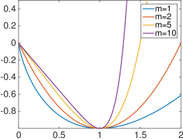
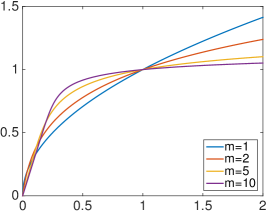
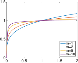
$e_{m}$	$\operatorname{Prox}^{\operatorname{KL}}_{\sigma e_{m}},\sigma=1$	$\operatorname{Prox}^{\operatorname{KL}}_{\sigma e_{m}},\sigma=3$

Fig. 5: Display of the graphs of functions $e_{m}$ and $\operatorname{Prox}^{\operatorname{KL}}_{\sigma e_{m}}$ for some values of $(\sigma,m)$.

Figure (6) shows illustration of the models in the case where either $b$ or $m$ is varying, thus producing a spatially varying flow. The initial distribution $p_{t=0}$ is computed as a white noise realization, where the pixels are independently and identically drawn according to a uniform distribution on $[0,1]$ (and then $p$ is normalized to unit mass).

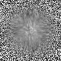
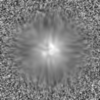
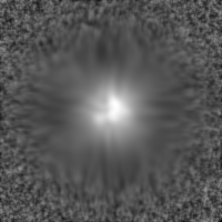
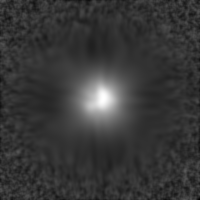
$t=0$	$t=10$	$t=20$	$t=30$	$t=40$

Fig. 6: Non-linear diffusion by gradient flow on the generalized entropies (36). Top row: fixed $m_{i}=1.4$ and varying weights $b_{i}\in[1,20]$ (1 in the boundary, 20 in the center). Bottom row: fixed $b_{i}=1$ and varying exponents $m_{i}\in[1,2]$ (1 in the boundary, $2$ in the center).

4.5 Non-convex Functionals

It is formally possible to apply Dykstra’s algorithm detailed in Section 3.4 to a non-convex function $f$, if one is able to compute in closed form the proximal operator (14) (which then might be a multi-valued map). Of course there is no hope for the resulting non-convex Dykstra’s algorithm to converge in general to the global minimizer of the non-convex optimization (11). Even worse, to the best of our knowledge, there is currently no proof that the non-convex Dykstra’s algorithm converges to a stationary point of the energy, even in the case of an Euclidean divergence. However, we found that applying Dykstra’s algorithm to non-convex functions works remarkably well in practice. Note that the closely related Douglas-Rachford (DR) algorithm is known to converge in some particular non-convex cases [5]. DR is known to perform very well on several non-convex optimization problems such as phase retrieval [8].

To test this non-convex setting, we replace the congestion box constraint (34) by the non-convex function

$$f(p)\stackrel{{\scriptstyle\mbox{\tiny def.}}}{{=}}\iota_{\{0,\kappa\}^{N}}+\langle w,\,p\rangle.$$ (39)

This function enforces that the thought after solution is binary, so that each value $p_{i}$ is in $\{0,\kappa\}$. The proximal operator of this non-convex function can be computed explicitly using

$$\forall\,i\in\{1,\ldots,N\},\quad\operatorname{Prox}_{\sigma\iota_{\{0,\kappa\}^{N}}}^{{\overline{\operatorname{KL}}}}(p)_{i}=\left\{\begin{array}[]{l}0\quad\text{if}\quad p_{i}<\kappa/e,\\ \{0,\kappa\}\quad\text{if}\quad p_{i}=\kappa/e,\\ \kappa\quad\text{if}\quad p_{i}>\kappa/e,\end{array}\right.$$

where $e=\exp(1)$. Note that $\operatorname{Prox}_{\sigma\iota_{\{0,\kappa\}^{N}}}^{{\overline{\operatorname{KL}}}}(p)_{i}$ is multi-valued at $p_{i}=\kappa/e$, and numerically one needs to chose one of the two values. Figure 7 shows a comparison of the evolutions obtained with the convex and non-convex functionals. The non-convex one suffers from binary noise artefacts, which could be partly due to the non-convexity, but also to the amplification of discretization errors by the proximal mapping which is not Lipschitz continuous.

$t=0$	$t=10$	$t=20$	$t=30$	$t=40$

Fig. 7: Display of crowd evolution for $\kappa=|\!|p_{t=0}|\!|_{\infty}$. Top row: convex function (34). Bottom row: non-convex function (39).

5 More General Functionals

In order to highlight the power of the proposed entropic regularization approach, we show here how to adapt the algorithm detailed in Section 3 in order to deal with more involved functionals. These functionals require the introduction of several couplings, which in turn necessitates to develop a generic iterative scaling procedure derived from Dykstra’s algorithm. This new method has its own interest, beyond the computation of Wasserstein gradient flows.

5.1 A Generic Diagonal Scaling Algorithm

In order to tackle a more general class of functions $f$, we consider here a generalization of problem (11) where one wants to optimize over a family $\pi=(\pi_{1},\ldots,\pi_{M})$ of $M$ couplings $\pi_{m}\in\mathbb{R}^{N\times N}$ a functional of the form

$$\underset{\pi\in(\mathbb{R}^{N\times N})^{M}}{\min}\;\operatorname{KL}_{\lambda}(\pi|\xi)+\varphi_{1}(\pi)+\varphi_{2}(\pi)\quad\text{where}\quad\left\{\begin{array}[]{l}\varphi_{1}(\pi)\stackrel{{\scriptstyle\mbox{\tiny def.}}}{{=}}\psi_{1}(\pi\mathds{1}),\\ \varphi_{2}(\pi)\stackrel{{\scriptstyle\mbox{\tiny def.}}}{{=}}\psi_{2}(\pi^{T}\mathds{1}),\end{array}\right.$$ (40)

where, for $\lambda\in\mathbb{R}_{+}^{M}$, $\operatorname{KL}_{\lambda}$ is the weighted KL divergence (see also (44))

$$\forall\,(\pi,\xi)\in(\mathbb{R}^{N\times N})^{M}\times(\mathbb{R}^{N\times N})^{M},\quad\operatorname{KL}_{\lambda}(\pi|\xi)=\sum_{m=1}^{M}\lambda_{m}\operatorname{KL}(\pi_{m}|\xi_{m})$$

and where we denoted, with a slight abuse of notations, the collection of left and right marginals as

$$\pi\mathds{1}=(\pi_{1}\mathds{1},\ldots,\pi_{M}\mathds{1})\in(\mathbb{R}^{N})^{M}\quad\text{and}\quad\pi^{T}\mathds{1}=(\pi_{1}^{T}\mathds{1},\ldots,\pi_{M}^{T}\mathds{1})\in(\mathbb{R}^{N})^{M}$$

and $\psi_{i}:(\mathbb{R}^{N})^{M}\rightarrow\mathbb{R}$ are convex functions for which one can compute the proximal operator $\operatorname{Prox}^{{\overline{\operatorname{KL}}}_{\lambda}}_{\psi_{i}}$ according to the ${\overline{\operatorname{KL}}}_{\lambda}$ divergence.

We wish to apply Dykstra’s iterations (24) and (25) to (40). This requires to compute the proximal operator of the functions $\varphi_{i}$. The following proposition details how to achieve this using the proximal operator of the functions $\psi_{i}$ alone.

Proposition 3.

We denote, for $i=1,2$, $\pi^{[i]}\stackrel{{\scriptstyle\mbox{\tiny def.}}}{{=}}\operatorname{Prox}^{\operatorname{KL}_{\lambda}}_{\varphi_{i}}(\pi)$. We denote, for $m=1,\ldots,M$, $\tilde{p}_{m}^{[1]}\stackrel{{\scriptstyle\mbox{\tiny def.}}}{{=}}\pi_{m}\mathds{1}$ and $\tilde{p}_{m}^{[2]}\stackrel{{\scriptstyle\mbox{\tiny def.}}}{{=}}\pi_{m}^{T}\mathds{1}$. One has

$$\forall\,m\in\{1,\ldots,M\},\quad\pi_{m}^{[1]} =\mathop{\operator@font diag}\nolimits\left(\frac{p_{m}^{[1]}}{\tilde{p}_{m}^{[1]}}\right)\pi_{m}\quad\text{and}\quad\pi_{m}^{[2]}=\pi_{m}\mathop{\operator@font diag}\nolimits\left(\frac{p_{m}^{[2]}}{\tilde{p}_{m}^{[2]}}\right)$$

$$\quad\text{where}\quad\forall\,i\in\{1,2\},\quad(p^{[i]})_{m} =\operatorname{Prox}^{{\overline{\operatorname{KL}}}_{\lambda}}_{\psi_{i}}\left((\tilde{p}^{[i]})_{m}\right).$$

Proof.

This corresponds to an application of formulas (49) and (50). ∎

The following proposition, which is similar to Proposition 2, explains how to implement the iterations of Dykstra’s algorithm using only multiplications with the kernels $(\xi_{m})_{m}$.

Proposition 4.

The iterates $\pi^{(\ell)}=(\pi_{1}^{(\ell)},\ldots,\pi_{M}^{(\ell)})$ of Dykstra’s algorithm can be written as

$$\forall\,m\in\{1,\ldots,M\},\quad\pi_{m}^{(\ell)}=\mathop{\operator@font diag}\nolimits(a_{m}^{(\ell)})\xi_{m}\mathop{\operator@font diag}\nolimits(b_{m}^{(\ell)})\quad\text{and}\quad z_{m}^{(\ell)}=u_{m}^{(\ell)}v_{m}^{(\ell),T}.$$

with the initialization

$$\forall\,m\in\{1,\ldots,M\},\quad a_{m}^{(0)}=b_{m}^{(0)}=u_{m}^{(0)}=v_{m}^{(0)}\stackrel{{\scriptstyle\mbox{\tiny def.}}}{{=}}\mathds{1}.$$

We define, $\forall\,m\in\{1,\ldots,M\}$,

$$\tilde{a}_{m}^{(\ell-1)} \stackrel{{\scriptstyle\mbox{\tiny def.}}}{{=}}a_{m}^{(\ell-1)}\odot u_{m}^{(\ell-2)}\quad\text{and}\quad\tilde{b}_{m}^{(\ell-1)}\stackrel{{\scriptstyle\mbox{\tiny def.}}}{{=}}b_{m}^{(\ell-1)}\odot v_{m}^{(\ell-2)},$$

$$(p_{m})_{m} \stackrel{{\scriptstyle\mbox{\tiny def.}}}{{=}}\operatorname{Prox}^{{\overline{\operatorname{KL}}}_{\lambda}}_{\psi_{[\ell]_{2}}}((\tilde{p}_{m})_{m})\quad\text{where}\quad\tilde{p}_{m}\stackrel{{\scriptstyle\mbox{\tiny def.}}}{{=}}\left\{\begin{array}[]{l}\tilde{a}_{m}^{(\ell-1)}\odot\xi_{m}(\tilde{b}_{m}^{(\ell-1)})\quad\text{if}\quad[\ell]_{2}=1,\\ \tilde{b}_{m}^{(\ell-1)}\odot\xi_{m}^{T}(\tilde{a}_{m}^{(\ell-1)})\quad\text{if}\quad[\ell]_{2}=2.\end{array}\right.$$

The update reads, $\forall\,m\in\{1,\ldots,M\}$,

$$a_{m}^{(\ell)} \stackrel{{\scriptstyle\mbox{\tiny def.}}}{{=}}\left\{\begin{array}[]{l}p_{m}\odot[\xi_{m}(\tilde{b}_{m}^{(\ell-1)})]^{-1}\quad\text{if}\quad[\ell]_{2}=1\\ \tilde{a}_{m}^{(\ell-1)}\quad\text{if}\quad[\ell]_{2}=2\end{array}\right.$$

$$b_{m}^{(\ell)} \stackrel{{\scriptstyle\mbox{\tiny def.}}}{{=}}\left\{\begin{array}[]{l}\tilde{b}_{m}^{(\ell-1)}\quad\text{if}\quad[\ell]_{2}=1\\ p_{m}\odot[\xi_{m}^{T}(\tilde{a}_{m}^{(\ell-1)})]^{-1}\quad\text{if}\quad[\ell]_{2}=2\end{array}\right.$$

$$u_{m}^{(\ell)} \stackrel{{\scriptstyle\mbox{\tiny def.}}}{{=}}u_{m}^{(\ell-2)}\odot\frac{a_{m}^{(\ell-1)}}{a_{m}^{(\ell)}}\quad\text{and}\quad v_{m}^{(\ell)}\stackrel{{\scriptstyle\mbox{\tiny def.}}}{{=}}v_{m}^{(\ell-2)}\odot\frac{b_{m}^{(\ell-1)}}{b_{m}^{(\ell)}}.$$

5.2 Wasserstein Attraction with Congestion

We now give a first concrete example of functional $f$ for which the formulation (40) should be used in place of (11).

Instead of advecting the mass of $p_{t}$ according to a fixed potential $w$ as it is considered in the functional (34), it is possible to make it evolve toward a “target” distribution $r\in\Sigma_{N}$ by minimizing the Wasserstein distance between $p_{t}$ and $r$. It thus consists in considering the gradient flow of the function

$$\forall\,p\in\Sigma_{N},\quad f(p)=W_{\gamma}(r,p)+h(p)+\iota_{\Sigma_{N}}(p),$$ (41)

where $h(p)$ is a function for which one can compute its ${\overline{\operatorname{KL}}}$ proximal operator as defined in (9).

We now denote $q\stackrel{{\scriptstyle\mbox{\tiny def.}}}{{=}}p_{t}$ the previous iterate, and aim at solving a single JKO step (10). It is not possible to compute in closed form the ${\overline{\operatorname{KL}}}$ proximal operator of the function $f$ defined in (41), so that the algorithm detailed in Section 3 is not directly applicable.

Instead, we re-formulate (10) as a KL minimization of the form (40) involving $M=2$ couplings $\pi=(\pi_{1},\pi_{2})\in(\mathbb{R}^{N\times N})^{2}$ and kernels $\xi=(\xi_{1},\xi_{2})\stackrel{{\scriptstyle\mbox{\tiny def.}}}{{=}}(e^{-c/\gamma},e^{-c/\gamma})$. This encodes implicitly the solution $p=\pi_{1}\mathds{1}=\pi_{2}\mathds{1}$ of (10) using the solution $\pi=(\pi_{1},\pi_{2})$ of (40) when introducing the functions

$$\psi_{1}(p_{1},p_{2}) =\iota_{\mathcal{D}}(p_{1},p_{2})+h(p_{1})\quad\text{where}\quad\mathcal{D}=\left\{(p_{1},p_{2})\;;\;p_{1}=p_{2}\right\},$$

$$\psi_{2}(p_{1},p_{2}) =\iota_{\{q,r\}}(p_{1},p_{2}),$$

and the weights $\lambda=(1,\tau)\in\mathbb{R}_{+}^{2}$. The following proposition details how to compute the proximal operator of these functionals. It is important to remind that that these functionals as well as their respective proximal operators operate on vectors of $\mathbb{R}^{N}$, not on couplings.

Proposition 5.

One has

$$\operatorname{Prox}^{{\overline{\operatorname{KL}}}_{\lambda}}_{\psi_{1}}(p_{1},p_{2}) =(p,p)\quad\text{where}\quad p=\operatorname{Prox}^{{\overline{\operatorname{KL}}}}_{\frac{1}{1+\tau}h}\left(p_{1}^{\frac{1}{1+\tau}}\odot p_{2}^{\frac{\tau}{1+\tau}}\right)$$ (42)

$$\operatorname{Prox}^{{\overline{\operatorname{KL}}}_{\lambda}}_{\psi_{2}}(p_{1},p_{2}) =(q,r)$$ (43)

Proof.

The computation of $\operatorname{Prox}^{{\overline{\operatorname{KL}}}_{\lambda}}_{\psi_{1}}$ follows from (47). The computation of $\operatorname{Prox}^{{\overline{\operatorname{KL}}}_{\lambda}}_{\psi_{2}}$ follows from (45). ∎

With these proximal maps at hands, and with the formula for the iterations detailed in Proposition 4, one can solve for each JKO step by computing the optimal $(\pi_{1},\pi_{2})$ using $q\stackrel{{\scriptstyle\mbox{\tiny def.}}}{{=}}p_{t}$ and then updating $p_{t+1}\stackrel{{\scriptstyle\mbox{\tiny def.}}}{{=}}\pi_{1}\mathds{1}=\pi_{2}\mathds{1}$.

Numerical Illustrations

In order to introduce some congestion, we consider here the function $h(p)=\iota_{[0,\kappa]^{N}}$, as in (34), and its KL proximal operator is computed as detailed in (35).

Figure 8 shows some examples of such a JKO flows computed on a rectangular grid of $N=100\times 100$ points. The right hand side column shows the target distribution $r$. Note that the flow $p_{t}$ typically does not converge toward $r$ as $t\rightarrow+\infty$, because of the congestion effect.

$t=0$	$t=10$	$t=20$	$t=30$	$t=40$	$r$

Fig. 8: Examples of gradient flows for the Wasserstein attraction toward the density $r$ displayed on the right column. The congestion parameter is set to $\kappa=|\!|p_{t=0}|\!|_{\infty}$.

5.3 Multiple Densities Evolutions

A natural extension of the JKO flow (8) is to describe the evolution of a finite family of densities $p_{t}=(p_{i,t})_{i}$ by minimizing a function $f((p_{i})_{i})$, where one defines the transport distance as the sum of independent Wasserstein distances

$$W_{\gamma}((p_{i})_{i},(q_{i})_{i})\stackrel{{\scriptstyle\mbox{\tiny def.}}}{{=}}\sum_{i}W_{\gamma}(p_{i},q_{i}).$$

The function $f$ thus introduce a coupling between densities during the evolution. For simplicity we consider in the following the case of $2$ densities.

Wasserstein pairwise attraction

We first consider the case where the coupling is a Wasserstein attraction between the two densities

$$f(p_{1},p_{2})=\alpha W(p_{1},p_{2})+h_{1}(p_{1})+h_{1}(p_{2})$$

where the functions $h_{i}$ are “simple” so that one can compute easily $\operatorname{Prox}_{h_{i}}^{{\overline{\operatorname{KL}}}}$.

Denoting $q=(q_{1},q_{2})\stackrel{{\scriptstyle\mbox{\tiny def.}}}{{=}}(p_{1,t},p_{2,t})$ the previous iterate at time $t$, the solution $p=p_{t+1}$ to the JKO step (10) can be written as

$$p=(p_{1},p_{2})=(\pi_{1}\mathds{1},\pi_{2}\mathds{1})=(\pi_{3}^{T}\mathds{1},\pi_{3}^{T}\mathds{1}),$$

where one needs to solve for $M=3$ couplings $(\pi_{1},\pi_{2},\pi_{3})$ the problem (40) with the functionals

$$\psi_{1}(a_{1},a_{2},a_{3}) =\iota_{\mathcal{D}}(a_{1},a_{3})+\iota_{\{q_{2}\}}(a_{2})+\frac{\tau}{\gamma}h_{1}(a_{1}),$$

$$\psi_{2}(a_{1},a_{2},a_{3}) =\iota_{\mathcal{D}}(a_{2},a_{3})+\iota_{\{q_{1}\}}(a_{1})+\frac{\tau}{\gamma}h_{2}(a_{2})$$

with KL weights $\lambda=(1,1,\tau\alpha)$. The proximal operators of these functions are easy to compute as detailed in the following proposition.

Proposition 4.

For $i\in\{1,2\}$, denoting $j=3-i\in\{1,2\}$, one has

$$(b_{m})_{m}=\operatorname{Prox}_{\psi_{i}}^{{\overline{\operatorname{KL}}}_{\lambda}}(a_{m})_{m}\quad\text{where}\quad b_{i}=b_{3}=\operatorname{Prox}_{h_{i}}(a_{i}^{\frac{1}{1+\tau\alpha}}\odot a_{3}^{\frac{\tau}{1+\tau\alpha}}),\quad b_{j}=q_{j}.$$

Proof.

The expression for $(b_{i},b_{3})$ is obtained by using (47). The expression for $b_{j}$ is obtained by using (45). ∎

In the numerical example, we used $h_{i}(p_{i})\stackrel{{\scriptstyle\mbox{\tiny def.}}}{{=}}\iota_{[0,\kappa]^{N}}(p_{i})+\langle w_{i},\,p_{i}\rangle$ for potentials $(w_{1},w_{2})\in\mathbb{R}^{N}\times\mathbb{R}^{N}$. The $\operatorname{KL}$ proximal operator of these functions can be computed as detailed in Proposition 2. Figure 9 displays the results obtained on a rectangular grid of $N=200\times 200$ points.

$t=0$	$t=10$	$t=20$	$t=30$	$t=40$

Fig. 9: Evolution with a pairwise attraction between two densities, with congestion parameter $\kappa=|\!|p_{1,t=0}|\!|_{\infty}=|\!|p_{2,t=0}|\!|_{\infty}$. Display of both $p_{1,t}$ (red) and $p_{2,t}$ (green), yellow indicates a mixing. Top row: $\alpha=1$. Bottom row: $\alpha=3$.

Summation couplings

Another way to introduce some interaction between $p_{1}$ and $p_{2}$ is to consider a coupling on the sum

$$f(p_{1},p_{2})\stackrel{{\scriptstyle\mbox{\tiny def.}}}{{=}}h(p_{1}+p_{2})+\langle p_{1},\,w_{1}\rangle+\langle p_{2},\,w_{2}\rangle.$$

for some function $h$ for which one can compute easily $\operatorname{Prox}_{h}^{\operatorname{KL}}$.

In this case, the solution $p=p_{t+1}$ to the JKO step (10) can be written as $p=(p_{1},p_{2})=(\pi_{1}\mathds{1},\pi_{2}\mathds{1})$ where the $M=2$ couplings $(\pi_{1},\pi_{2})$ solves problem (40) with the functionals

$$\psi_{1}(a_{1},a_{2}) =\frac{\tau}{\gamma}f(a_{1},a_{2}),$$

$$\psi_{2}(a_{1},a_{2}) =\iota_{\{q_{1},q_{2}\}}(a_{1},a_{2})$$

and weights $\lambda=(1,1)$. The proximal operators of the functions are easy to compute as detailed in the following proposition.

Proposition 5.

One has

$$\operatorname{Prox}_{\psi_{1}}^{{\overline{\operatorname{KL}}}_{\lambda}}(a_{1},a_{2}) =\frac{\operatorname{Prox}_{\frac{\tau}{\gamma}h}(\tilde{a}_{1}+\tilde{a}_{2})}{\tilde{a}_{1}+\tilde{a}_{2}}\odot(\tilde{a}_{1},\tilde{a}_{2})$$

$$\operatorname{Prox}_{\psi_{2}}^{{\overline{\operatorname{KL}}}_{\lambda}}(a_{1},a_{2}) =(q_{1},q_{2}).$$

where $\tilde{a}_{i}=a_{i}\odot e^{-\frac{\tau}{\gamma}w_{i}}$

Proof.

The expression for $\operatorname{Prox}_{\psi_{1}}^{{\overline{\operatorname{KL}}}_{\lambda}}$ is obtained by combining (46) and (49). The expression for $\operatorname{Prox}_{\psi_{2}}^{{\overline{\operatorname{KL}}}_{\lambda}}$ is obtained by using (45). ∎

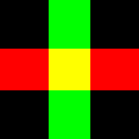
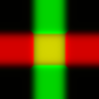
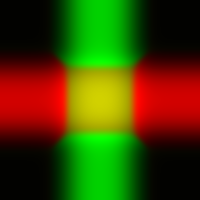
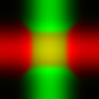
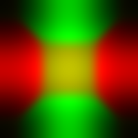
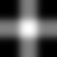
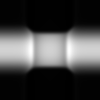
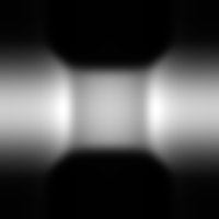
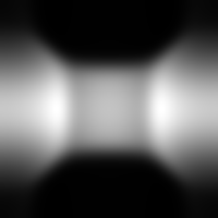
$t=0$	$t=10$	$t=20$	$t=30$	$t=40$

Fig. 10: Evolution with a summation coupling $E(p_{1}+p_{2})$. Top row: display of both $p_{1}$ (red) and $p_{2}$ (green), yellow indicates a mixing. Middle row: display of $p_{1}+p_{2}$, which evolves according to a linear heat diffusion. Bottom row: display of $p_{1}$.

As a first example, we consider an entropic coupling $h=E$, with $w_{1}=w_{2}=0$. Its proximal operator is computed in (37). A formal computation shows that, for the Euclidean $W_{2}$ transport on $\mathbb{R}^{d}$, the corresponding discrete JKO steps (8) is intended at approximating the non-linear PDE over $p_{t}=(p_{1,t},p_{2,t})$

$$\forall\,i\in\{1,2\},\quad\forall\,t>0,\quad\partial_{t}p_{i,t}=\operatorname{div}\left(\frac{p_{i,t}}{p_{1,t}+p_{2,t}}\nabla p_{i,t}\right).$$

This shows that while $p_{t}$ follows a non-linear coupled diffusion, $p_{1,t}+p_{2,t}$ follows a linear heat diffusion. Figure 10 shows a numerical illustration on a regular grid of $N=200\times 200$ points.

As a second example, we consider a congestion coupling $h=\iota_{[0,\kappa]^{N}}$. Its proximal operator is computed in (35). Figure 11 shows a numerical illustration on a regular grid of $N=200\times 200$ points. It shows two densities, initially supported on non-overlapping squares, moving in opposite directions under potentials $(w_{1},w_{2})$ such that $\nabla w_{1}=(1,0)^{T}$ and $\nabla w_{2}=(-1,0)^{T}$ (constant horizontal gradients). A congestion shock is created by the overlap of the densities, which in turn forces the support of the densities to be deformed and vertically enlarged.

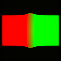
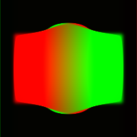
$t=0$	$t=10$	$t=20$	$t=30$	$t=40$

Fig. 11: Evolution with a summation coupling $\iota_{[0,\kappa]^{N}}(p_{1}+p_{2})$ where $\kappa=|\!|p_{1,t=0}|\!|_{\infty}=|\!|p_{2,t=0}|\!|_{\infty}$. Top row: display of both $p_{1,t}$ (red) and $p_{2,t}$ (green), yellow indicates a mixing. Middle row: display of $p_{1,t}+p_{2,t}$. Bottom row: display of $p_{1,t}$.

Discussion and Conclusion

In this paper, we have presented a novel algorithm to compute approximate discrete gradient flows according to an entropic smoothing of the Wasserstein distance. The main interest of the method is its speed, simplicity and versatility. This is achieved because the iterations only require (beside pointwise multiplications, divisions and exponentiations) to compute the successive applications of a “convolution-like” operator corresponding to the Gibbs kernel associated to the metric.

A natural question is to explore whether the discrete flow defined by (8) has a continuous limit when $\tau_{t}=\tau\rightarrow 0$. If one uses a fixed $\gamma_{t}=\gamma>0$, this is not the case, because $W_{\gamma}$ does not satisfies $W_{\gamma}(p,p)=0$. More precisely, one has that

$$\underset{q}{\operatorname{argmin}}\;W_{\gamma}(p,q)=\xi\left(\frac{p}{\xi^{T}(p)}\right),$$

so that the limit for small $\tau$ of $p_{t+1}$ defined by (8) is a blurred (i.e. multiplied by $\xi$) version of $p_{t}$. Instead of using a fixed value for $\gamma_{t}$, choosing $\gamma_{t}=\gamma(\tau_{t})$ for some carefully chosen function of $\tau_{t}$ could allow the discrete flow to converge to the usual Wasserstein flow. We leave the analysis of this asymptotic setting to a future work.

Aknowledgements

This work has been supported by the European Research Council (ERC project SIGMA-Vision). I would like to acknowledge stimulating discussions with Marco Cuturi, Justin Solomon, Jean-David Benamou, Guillaume Carlier and Quentin Merigot. I would like to thank Guillaume Carlier for suggesting to apply the method to multiple densities (Section 5.3). I would like to thank Jean-Marie Mirebeau for giving me access to his code for anisotropic diffusion. I would like to thank Antonin Chambolle and Jalal Fadili for suggesting me the proof strategy of Proposition 1.

Appendix A KL Proximal Calculus

The following proposition details some useful property of the ${\overline{\operatorname{KL}}}$ proximal operator (9). This enables a powerful “proximal calculus” by combining these rules, which eases and simplifies the implementation of the algorithms. Note that we also consider generalized KL divergence over sets $(p_{1},\ldots,p_{M})$ of $M$ densities according to some weight $\lambda\in\mathbb{R}_{+}^{M}$

$$\forall\,(p_{m})_{m},(q_{m})_{m},\quad{\overline{\operatorname{KL}}}_{\lambda}((p_{m})_{m}|(q_{m})_{m})\stackrel{{\scriptstyle\mbox{\tiny def.}}}{{=}}\sum_{m=1}^{M}\lambda_{m}{\overline{\operatorname{KL}}}(p_{m}|q_{m}).$$ (44)

Proposition 6.

For $f(p_{1},\ldots,p_{M})\stackrel{{\scriptstyle\mbox{\tiny def.}}}{{=}}\iota_{\{(q_{1},\ldots,q_{M})\}}(p_{1},\ldots,p_{M})$, one has

$$\operatorname{Prox}_{f}^{{\overline{\operatorname{KL}}}_{\lambda}}(p_{1},\ldots,p_{M})=(q_{1},\ldots,q_{M}).$$ (45)

For $f(p_{1},\ldots,p_{M})\stackrel{{\scriptstyle\mbox{\tiny def.}}}{{=}}h(p_{1},\ldots,p_{M})+\sum_{i=1}^{M}\langle w_{i},\,p_{i}\rangle$, one has

$$\operatorname{Prox}_{f}^{{\overline{\operatorname{KL}}}_{\lambda}}(p_{1},\ldots,p_{M})=\operatorname{Prox}_{h}^{{\overline{\operatorname{KL}}}_{\lambda}}(p_{1}\odot e^{-w_{1}/\lambda_{1}},\ldots,p_{M}\odot e^{-w_{M}/\lambda_{M}}).$$ (46)

For $f(p_{1},\ldots,p_{M})\stackrel{{\scriptstyle\mbox{\tiny def.}}}{{=}}\iota_{\mathcal{D}}(p_{1},\ldots,p_{M})+h(p_{1},\ldots,p_{M})$ where

$$\mathcal{D}\stackrel{{\scriptstyle\mbox{\tiny def.}}}{{=}}\left\{(p_{1},\ldots,p_{M})\;;\;p_{1}=\ldots=p_{M}\right\},$$

one has

$$\operatorname{Prox}_{f}^{{\overline{\operatorname{KL}}}_{\lambda}}(p_{1},\ldots,p_{M})=(p,\ldots,p)\!\quad\text{where}\quad\!p=\operatorname{Prox}_{\frac{1}{\sum_{i}\lambda_{i}}\tilde{h}}^{\operatorname{KL}}\left(p_{1}^{\tilde{\lambda}_{1}}\odot\ldots\odot p_{M}^{\tilde{\lambda}_{M}}\right),$$ (47)

where we denoted $\tilde{\lambda}_{i}\stackrel{{\scriptstyle\mbox{\tiny def.}}}{{=}}\lambda_{i}/\sum_{j}\lambda_{j}$ and $\tilde{h}(p)=h(p,\ldots,p)$.
For $f(p_{1},\ldots,p_{M})\stackrel{{\scriptstyle\mbox{\tiny def.}}}{{=}}h(p_{1}+\ldots+p_{M})$ and $\lambda\stackrel{{\scriptstyle\mbox{\tiny def.}}}{{=}}(1,\ldots,1)$, one has

$$\operatorname{Prox}_{f}^{{\overline{\operatorname{KL}}}_{\lambda}}(p_{1},\ldots,p_{M})=\frac{\operatorname{Prox}_{h}^{{\overline{\operatorname{KL}}}}(p_{1}+\ldots+p_{M})}{p_{1}+\ldots+p_{M}}(p_{1},\ldots,p_{M})$$ (48)

We define $f(\pi_{1},\ldots,\pi_{M})\stackrel{{\scriptstyle\mbox{\tiny def.}}}{{=}}h(\pi_{1}\mathds{1},\ldots,\pi_{M}\mathds{1})$. We denote

$$\forall\,m\in\{1,\ldots,M\},\quad p_{m}\stackrel{{\scriptstyle\mbox{\tiny def.}}}{{=}}\pi_{m}\mathds{1}\quad\text{and}\quad(\tilde{p}_{1},\ldots,\tilde{p}_{M})\stackrel{{\scriptstyle\mbox{\tiny def.}}}{{=}}\operatorname{Prox}_{h}^{{\overline{\operatorname{KL}}}_{\lambda}}(p_{1},\ldots,p_{M}).$$

One has

$$\operatorname{Prox}_{f}^{\operatorname{KL}_{\lambda}}(\pi_{1},\ldots,\pi_{M})=\left(\mathop{\operator@font diag}\nolimits\left(\frac{\tilde{p}_{m}}{p_{m}}\right)~\pi\right)_{m}$$ (49)

We define $f(\pi_{1},\ldots,\pi_{M})\stackrel{{\scriptstyle\mbox{\tiny def.}}}{{=}}h(\pi_{1}^{T}\mathds{1},\ldots,\pi_{M}^{T}\mathds{1})$. We denote

$$\forall\,m\in\{1,\ldots,M\},\quad p_{m}\stackrel{{\scriptstyle\mbox{\tiny def.}}}{{=}}\pi_{m}^{T}\mathds{1}\quad\text{and}\quad(\tilde{p}_{1},\ldots,\tilde{p}_{M})\stackrel{{\scriptstyle\mbox{\tiny def.}}}{{=}}\operatorname{Prox}_{h}^{{\overline{\operatorname{KL}}}_{\lambda}}(p_{1},\ldots,p_{M}).$$

One has

$$\operatorname{Prox}_{f}^{\operatorname{KL}_{\lambda}}(\pi_{1},\ldots,\pi_{M})=\left(\pi\mathop{\operator@font diag}\nolimits\left(\frac{\tilde{p}_{m}}{p_{m}}\right)\right)_{m}$$ (50)

Proof.

Proof of (45).   This is straightforward.
Proof of (46).   If follows from the relation

$${\overline{\operatorname{KL}}}_{\lambda}((q_{1},\ldots,q_{M})|(p_{1},\ldots,p_{M}))+\sum_{i=1}^{M}\langle w_{i},\,q_{i}\rangle$$

$$= {\overline{\operatorname{KL}}}_{\lambda}((q_{1},\ldots,q_{M})|(p_{1}\odot e^{-w_{1}/\lambda_{1}},\ldots,p_{M}\odot e^{-w_{M}/\lambda_{M}})).$$

Proof of (47).   We denote $(q_{m})_{m}\stackrel{{\scriptstyle\mbox{\tiny def.}}}{{=}}\operatorname{Prox}^{{\overline{\operatorname{KL}}}_{\lambda}}_{\psi_{1}}((p_{m})_{m})$, so that $q=q_{1}=\ldots=q_{M}$ solves

$$\underset{q}{\min}\;\sum_{m}\lambda_{m}{\overline{\operatorname{KL}}}(q|p_{m})+\tilde{h}(q).$$

The result follow from the relation

$$\sum_{m}\lambda_{m}{\overline{\operatorname{KL}}}(q|p_{m})=\textstyle\left(\sum_{m}\lambda_{m}\right){\overline{\operatorname{KL}}}\left(q|p_{1}^{\tilde{\lambda}_{1}}\odot\ldots\odot p_{M}^{\tilde{\lambda}_{M}}\right).$$

Proof of (48).   Denoting $(q_{m})_{m}=\operatorname{Prox}_{f}^{{\overline{\operatorname{KL}}}_{\lambda}}((p_{m})_{m})$, the first order optimality condition for $\operatorname{Prox}_{f}^{{\overline{\operatorname{KL}}}_{\lambda}}$ reads

$$\forall\,m\in\{1,\ldots,M\},\quad\log\left(\frac{q_{m}}{p_{m}}\right)+u=0$$

where $u\in\partial h(p_{1}+\ldots+p_{M})$. respectively summing and subtracting these equations lead to

$$q_{1}+\ldots+q_{M}=\operatorname{Prox}_{h}(p_{1}+\ldots+p_{M})\quad\text{and}\quad\frac{q_{1}}{p_{1}}=\ldots=\frac{q_{m}}{p_{m}}.$$

Solving for $(q_{1},\ldots,q_{m})$ in these equations leads to the desired solution.
Proof of (49).   The first order condition for $\tilde{\pi}$ being a solution of (14) states the existence of $(z_{m})_{m}\in\partial f(\tilde{p}_{1},\ldots,\tilde{p}_{M})$ where $\tilde{p}_{m}=\tilde{\pi}_{m}\mathds{1}$ such that

$$\lambda_{m}\log\left(\frac{\tilde{\pi}_{m}}{\pi_{m}}\right)+z_{m}\mathds{1}^{T}=0\;\Rightarrow\;\tilde{\pi}_{m}=\mathop{\operator@font diag}\nolimits(e^{-z_{m}/\lambda_{m}})\pi_{m}\;\Rightarrow\;\tilde{p}_{m}=\mathop{\operator@font diag}\nolimits(e^{-z_{m}/\lambda_{m}})p_{m},$$

which corresponds to the first order condition for $(\tilde{p}_{m})_{m}$ being a solution of (9) for the function $h$, i.e.

$$(\tilde{p}_{m})_{m}=\operatorname{Prox}_{h}^{{\overline{\operatorname{KL}}}}((p_{m})_{m}).$$

Finally, one obtains

$$\tilde{\pi}_{m}=\mathop{\operator@font diag}\nolimits(e^{-z_{m}/\lambda_{m}})\pi_{m}=\mathop{\operator@font diag}\nolimits\left(\frac{\tilde{p}_{m}}{p_{m}}\right)\pi_{m}$$

and hence the desired result.
Proof of (50).   It is obtained by transposing formula (49). ∎

References

- [1] M. Agueh. Existence of solutions to degenerate parabolic equations via the Monge-Kantorovich theory. PhD thesis, Georgia Institute of Technology, USA, 2002.
- [2] M. Agueh and M. Bowles. One-dimensional numerical algorithms for gradient flows in the -Wasserstein spaces. Acta Applicandae Mathematicae, 125(1):121–134, 2013.
- [3] M. Agueh and G. Carlier. Barycenters in the Wasserstein space. SIAM J. on Mathematical Analysis, 43(2):904–924, 2011.
- [4] L. Ambrosio, N. Gigli, and G. Savaré. Gradient flows: in metric spaces and in the space of probability measures. Springer, 2006.
- [5] A. Artacho, Borwein F. J., and J. M. Global convergence of a non-convex douglas-rachford iteration. J. Global Optimization, 57(3):1–17, 2012.
- [6] H. H. Bauschke and P. L. Combettes. A Dykstra-like algorithm for two monotone operators. Pacific Journal of Optimization, 4(3):383–391, 2008.
- [7] H. H. Bauschke and P. L. Combettes. Convex Analysis and Monotone Operator Theory in Hilbert Spaces. Springer-Verlag, New York, 2011.
- [8] H. H. Bauschke, P. L. Combettes, and D. R. Luke. Phase retrieval, error reduction algorithm, and Fienup variants: A view from convex optimization. J. Opt. Soc. Am. A, 19(7):1334–1345, 2002.
- [9] H. H. Bauschke and A. S. Lewis. Dykstra’s algorithm with Bregman projections: a convergence proof. Optimization, 48(4):409–427, 2000.
- [10] J.-D. Benamou and Y. Brenier. A computational fluid mechanics solution of the Monge-Kantorovich mass transfer problem. Numerische Mathematik, 84(3):375–393, 2000.
- [11] J-D. Benamou, G. Carlier, M. Cuturi, L. Nenna, and G. Peyré. Iterative bregman projections for regularized transportation problems. to appear in SIAM J. Sci. Comp., 2015.
- [12] J-D. Benamou, G. Carlier, Q. Mérigot, and E. Oudet. Discretization of functionals involving the Monge-Ampère operator. Preprint arXiv:1408.4536, 2014.
- [13] J. Bigot and T. Klein. Consistent estimation of a population barycenter in the Wasserstein space. Preprint arXiv:1212.2562, 2012.
- [14] A. Blanchet, V. Calvez, and J. A Carrillo. Convergence of the mass-transport steepest descent scheme for the subcritical patlak-keller-segel model. SIAM Journal on Numerical Analysis, 46(2):691–721, 2008.
- [15] A. Blanchet and G. Carlier. Optimal transport and Cournot-Nash equilibria. arXiv preprint arXiv:1206.6571, 2012.
- [16] N. Bonneel, M. van de Panne, S. Paris, and W. Heidrich. Displacement interpolation using Lagrangian mass transport. ACM Transactions on Graphics (SIGGRAPH ASIA’11), 30(6), 2011.
- [17] M. Botsch, L. Kobbelt, M. Pauly, P. Alliez, and B. Levy. Polygon Mesh Processing. Taylor & Francis, 2010.
- [18] L. M. Bregman. The relaxation method of finding the common point of convex sets and its application to the solution of problems in convex programming. USSR computational mathematics and mathematical physics, 7(3):200–217, 1967.
- [19] L.M. Bregman, Y. Censor, and S. Reich. Dykstra’s algorithm as the nonlinear extension of Bregman’s optimization method. Journal of Convex Analysis, 6:319–333, 1999.
- [20] Y. Brenier. The least action principle and the related concept of generalized flows for incompressible perfect fluids. J. of the AMS, 2:225–255, 1990.
- [21] C.J. Budd, M.J.P. Cullen, and E.J. Walsh. Monge-Ampère based moving mesh methods for numerical weather prediction, with applications to the eady problem. Journal of Computational Physics, 236:247–270, 2013.
- [22] M. Burger, J. A. Carrillo, and M-T. Wolfram. A mixed finite element method for nonlinear diffusion equations. Kinetic and Related Models, 3(1):59–83, 2010.
- [23] M. Burger, M. Franeka, and C-B. Schonlieb. Regularised regression and density estimation based on optimal transport. Appl. Math. Res. Express, 2:209–253, 2012.
- [24] J. A. Carrillo, A. Chertock, and Y. Huang. A finite-volume method for nonlinear nonlocal equations with a gradient flow structure. Communications in Computational Physics, 17:233–258, 1 2015.
- [25] J. A Carrillo and J. S. Moll. Numerical simulation of diffusive and aggregation phenomena in nonlinear continuity equations by evolving diffeomorphisms. SIAM Journal on Scientific Computing, 31(6):4305–4329, 2009.
- [26] Y. Censor and S. Reich. The Dykstra algorithm with Bregman projections. Communications in Applied Analysis, 2:407–419, 1998.
- [27] A. Chambolle and T. Pock. On the ergodic convergence rates of a first-order primal-dual algorithm. preprint, 2014.
- [28] P. G. Ciarlet. Introduction to Numerical Linear Algebra and Optimisation. Cambridge University Press, Cambridge, 1989. Originally published in French under the title, Introduction à l’analyse numérique matricielle et à l’optimisation in 1982.
- [29] K. Crane, C. Weischedel, and M. Wardetzky. Geodesics in heat: A new approach to computing distance based on heat flow. ACM Trans. Graph., 32(5):152:1–152:11, October 2013.
- [30] I. Csiszár. -divergence geometry of probability distributions and minimization problems. Ann. Probability, 3:146–158, 1975.
- [31] M. Cuturi. Sinkhorn distances: Lightspeed computation of optimal transport. In Advances in Neural Information Processing Systems (NIPS) 26, pages 2292–2300, 2013.
- [32] M. Cuturi and A. Doucet. Fast computation of Wasserstein barycenters. In Proceedings of the 31st International Conference on Machine Learning (ICML), JMLR W&CP, volume 32, 2014.
- [33] T. A. Davis. Direct Methods for Sparse Linear Systems. SIAM, 2006.
- [34] W. E. Deming and F. F. Stephan. On a least squares adjustment of a sampled frequency table when the expected marginal totals are known. Annals Mathematical Statistics, 11(4):427–444, 1940.
- [35] R. Deriche. Recursively implementing the Gaussian and its derivatives. Technical Report RR-1893, INRIA, 1993.
- [36] R. L. Dykstra. An iterative procedure for obtaining -projections onto the intersection of convex sets. Ann. Probab., 13(3):975–984, 1985.
- [37] J. Eckstein. Nonlinear proximal point algorithms using Bregman functions, with applications to convex programming. Mathematics of Operations Research, 18(1):202–226, 1993.
- [38] M. Erbar. The heat equation on manifolds as a gradient flow in the Wasserstein space. Annales de l’Institut Henri Poincaré, Probabilités et Statistiques, 46(1):1–23, 2010.
- [39] J. Fehrenbach and J-M. Mirebeau. Sparse non-negative stencils for anisotropic diffusion. Journal of Mathematical Imaging and Vision, 49(1):123–147, 2014.
- [40] A. Figalli. The optimal partial transport problem. Arch. Ration. Mech. Anal., 195(2):533–560, 2010.
- [41] U. Frisch, S. Matarrese, R. Mohayaee, and A. Sobolevski. Monge-Ampere-Kantorovitch (MAK) reconstruction of the early universe. Nature, 417(260), 2002.
- [42] K. Jonathan and R. J. McCann. Insights into capacity constrained optimal transport. Proc. Natl. Acad. Sci. USA, 110:10064–10067, 2013.
- [43] R. Jordan, D. Kinderlehrer, and O. Otto. The variational formulation of the Fokker-Planck equation. SIAM journal on mathematical analysis, 29(1):1–17, 1998.
- [44] L. Kantorovich. On the transfer of masses (in russian). Doklady Akademii Nauk, 37(2):227–229, 1942.
- [45] D. Kinderlehrer and N. J Walkington. Approximation of parabolic equations using the Wasserstein metric. ESAIM: Mathematical Modelling and Numerical Analysis, 33(04):837–852, 1999.
- [46] K.C. Kiwiel. Proximal minimization methods with generalized Bregman functions. SIAM J. Control Optim., 35(4):1142–1168, 1997.
- [47] C. Leonard. A survey of the Schrodinger problem and some of its connections with optimal transport. Discrete Contin. Dyn. Syst. A, 34(4):1533–1574, 2014.
- [48] D. Matthes and H. Osberger. Convergence of a variational lagrangian scheme for a nonlinear drift diffusion equation. Preprint arXiv:1301.0747, 2014.
- [49] B. Maury, A. Roudneff-Chupin, and F. Santambrogio. A macroscopic crowd motion model of gradient flow type. Mathematical Models and Methods in Applied Sciences, 20(10):1787–1821, 2010.
- [50] Y. Nesterov, A. Nemirovskii, and Y. Ye. Interior-point polynomial algorithms in convex programming, volume 13. SIAM, 1994.
- [51] F. Otto. The geometry of dissipative evolution equations: the porous medium equation. Communications in partial differential equations, 26(1-2):101–174, 2001.
- [52] N. Papadakis, G. Peyré, and E. Oudet. Optimal transport with proximal splitting. SIAM Journal on Imaging Sciences, 7(1):212–238, 2014.
- [53] B. Pass. On the local structure of optimal measures in the multi-marginal optimal transportation problem. Calc. Var. Partial Differential Equations, 43(3-4):529–536, 2012.
- [54] Y. Rubner, C. Tomasi, and L.J. Guibas. The earth mover’s distance as a metric for image retrieval. International Journal of Computer Vision, 40(2), 2000.
- [55] L. Ruschendorf and W. Thomsen. Closedness of sum spaces and the generalized Schrodinger problem. Theory of Probability and its Applications, 42(3):483–494, 1998.
- [56] E. Schrodinger. Uber die umkehrung der naturgesetze. Sitzungsberichte Preuss. Akad. Wiss. Berlin. Phys. Math., 144:144–153, 1931.
- [57] J.A. Sethian. Level Sets Methods and Fast Marching Methods. Cambridge University Press, 2nd edition, 1999.
- [58] R. Sinkhorn. A relationship between arbitrary positive matrices and doubly stochastic matrices. Ann. Math. Statist., 35:876–879, 1964.
- [59] R. Sinkhorn. Diagonal equivalence to matrices with prescribed row and column sums. Amer. Math. Monthly, 74:402–405, 1967.
- [60] R. Sinkhorn and P . Knopp. Concerning nonnegative matrices and doubly stochastic matrices. Pacific J. Math., 21:343–348, 1967.
- [61] M. V. Solodov and B. F. Svaiter. An inexact hybrid generalized proximal point algorithm and some new results on the theory of Bregman functions. Mathematics of Operations Research, 25(2):214–230, 2000.
- [62] J. Solomon, F. de Goes, G. Peyré, M. Cuturi, A. Butscher, A. Nguyen, T. Du, and L. Guibas. Convolutional Wasserstein distances: Efficient optimal transportation on geometric domains. Preprint, 2015.
- [63] S. R. S. Varadhan. On the behavior of the fundamental solution of the heat equation with variable coefficients. Communications on Pure and Applied Mathematics, 20(2):431–455, 1967.
- [64] C. Villani. Topics in Optimal Transportation. Graduate Studies in Mathematics Series. American Mathematical Society, 2003.
- [65] H. Wang and A. Banerjee. Bregman alternating direction method of multipliers. preprint arXiv:1306.3203, 2014.
- [66] J. Weickert. Anisotropic Diffusion in Image Processing. Teubner, Stuttgart, 1998.
- [67] M. Westdickenberg and J. Wilkening. Variational particle schemes for the porous medium equation and for the system of isentropic Euler equations. ESAIM: Mathematical Modelling and Numerical Analysis, 44(1):133–166, 2010.
- [68] G-S. Xia, S. Ferradans, G. Peyré, and J-F. Aujol. Synthesizing and mixing stationary Gaussian texture models. SIAM Journal on Imaging Sciences, 7(1):476–508, 2014.