Spatio-temporal Video Parsing for
Abnormality Detection

Abstract

Abnormality detection in video poses particular challenges due to the infinite size of the class of all irregular objects and behaviors. Thus no (or by far not enough) abnormal training samples are available and we need to find abnormalities in test data without actually knowing what they are. Nevertheless, the prevailing concept of the field is to directly search for individual abnormal local patches or image regions independent of another. To address this problem, we propose a method for joint detection of abnormalities in videos by spatio-temporal video parsing. The goal of video parsing is to find a set of indispensable normal spatio-temporal object hypotheses that jointly explain all the foreground of a video, while, at the same time, being supported by normal training samples. Consequently, we avoid a direct detection of abnormalities and discover them indirectly as those hypotheses which are needed for covering the foreground without finding an explanation for themselves by normal samples. Abnormalities are localized by MAP inference in a graphical model and we solve it efficiently by formulating it as a convex optimization problem. We experimentally evaluate our approach on several challenging benchmark sets, improving over the state-of-the-art on all standard benchmarks both in terms of abnormality classification and localization.

1 Introduction

With the rapid growth of video data, there is an increasing need not only for recognition of objects and their behavior, but in particular for detecting the rare, interesting occurrences of unusual objects or suspicious behavior in the large body of ordinary data. Finding such abnormalities in videos is crucial for applications ranging from automatic quality control to visual surveillance. Due to the large within-class variability, recognizing normal objects is already difficult. Abnormality detection in crowded scenes, however, features the additional challenge that there exist infinitely many ways for an object to appear in unusual context (irregular object instance) or to behave abnormally (unusual activity). Most of these abnormal instances are beforehand unknown, as this would for instance require predicting all the ways somebody could cheat or break a law. It is therefore simply impossible to learn a model for all that is abnormal or irregular. Consequently, recent work on abnormality detection [1] has focused on a setting where the training data contains only normal visual patterns. Thus a discriminative approach cannot be employed to directly localize irregularities in these benchmark datasets. But how can we find an abnormality without knowing what to look for? In spite of this fundamental problem, the main paradigm in abnormality detection is at present to independently classify individual video patches [2, 3] or regions [4].

If we want to avoid the ill-posed problem of having to decide locally and separately about the abnormality of each image region, we need to abandon the standard approach of object detection, which aims at detecting all objects in a scene independently from one another. Since abnormality detection is typically concerned with videos from a static camera as in surveillance or industrial inspection, robust background subtraction algorithms [5] can be used for foreground/background segregation. Our goal is then to find a set of spatio-temporal object hypotheses that jointly explain all foreground pixels. This means that normal object hypotheses, which can be learned from the training data, are spread over the spatio-temporal volume of a video in order to cover foreground pixels, while protruding into the background as little as possible. These hypotheses need to explain the appearance and behavior of the underlying video regions. As objects are mutually overlapping in crowded scenes, the spatio-temporal placement of the object hypotheses can only be determined jointly. Thus, our aim is to simultaneously select those object hypotheses, which are necessary for explaining the foreground and to identify for each selected hypothesis the best matching instance from the set of all normal training samples. Abnormal objects are then those hypotheses which are required for explaining the foreground, but which themselves cannot be explained by a normal training sample. Video parsing jointly infers all necessary object hypotheses, so that we can indirectly discover all abnormal objects present in a scene without actually knowing what to look for.

Our video parsing approach consists of two stages. In the first phase, we detect a large number of object candidates in each video frame and then group them temporally into spatio-temporal object hypotheses. This shortlist of hypotheses is a superset of all candidates that might be eventually needed for parsing the video, i.e., it has a low false negative and high false positive rate. The object candidates in individual frames are obtained by running a discriminative background classifier and keeping only those patterns which are very unlikely to be background. Subsequently, object candidates in individual frames are linked temporally according to their motion cues so as to establish the shortlist of spatio-temporal object hypotheses. In the second phase of video parsing, the goal is to select hypotheses from the shortlist that can explain the foreground, and to simultaneously find normal object instances that match those hypotheses. We formulate this as an inference problem in a graphical model whose goal is to maximize the probability of the foreground explanation in a video. The inference in the graphical model is cast as a convex optimization problem where the unknown variables indicate both, the selection of hypotheses from the shortlist and their corresponding normal object prototypes learned from the training videos. Correspondences between hypotheses and normal object prototypes are based upon their shape, location as well as their appearance and behavior. The probability of abnormality of each hypothesis necessary for explaining the foreground is then calculated using the results of inference. Beside identifying abnormal objects, video parsing also computes per-pixel probability of abnormality, which effectively segments abnormalities without having any training samples for them.

We evaluate our approach on novel benchmark datasets for abnormality detection that feature highly crowded scenes. As an example, the UCSD ped1 and ped2 anomaly detection and localization datasets [1] contain busy walkways teeming with walking pedestrians. Abnormalities are not staged, but they occur spontaneously and correspond to unusual objects (e.g., vehicles in a pedestrian zone) or behaviors (e.g., a person cycling across walkways) in the scene. The training data features only normal patterns with large intra-class variability, whereas the test set consists of normal and abnormal instances. Due to the small resolution of videos (a person in the scene is on average only $20$ pixels tall) and heavy occlusion between objects in the scene, learning models of visual patterns is difficult. We also increase the future utility of the UCSD ped1 dataset by completing the pixel-wise ground-truth annotation for all videos in the test set that previously existed only for a small subset. The experimental results show a significant performance gain of our spatio-temporal video parsing approach in comparison to other state-of-the-art methods for abnormality detection.

2 Related Work

We discuss here the previous work on abnormality detection in videos. The related problem of object recognition and tracking in crowded scenes [6, 7] aims at recognizing and tracking objects of a known class in a scene, whereas our goal is to detect abnormal objects, all of them being instances of an unknown class. Therefore, object recognition and tracking are beyond the scope of this paper and the details on these topics can be found in [8]. Majority of the work on abnormality detection relies on the extraction of semi-local features from video [9, 10, 11, 12, 13], that are then used to train a normalcy model. Abnormalities are detected if the normalcy model does not fit the data. Some approaches [14, 4] are based on manually specifying constraints that define the condition of normalcy, whereas other methods [3, 15, 16, 17, 18, 19] learn the normalcy model directly from data in unsupervised way.

The approach of Adam et al. [20] focuses on individual activities occurring only in selected parts of a scene. Kim and Grauman [21] detect abnormalities using a spatio-temporal Markov random field that adapts to abnormal activities in videos. Loy et al. [22] use active learning methodology to integrate human feedback into the detection of abnormal events and behaviors. Unsupervised topic models are used for detection of abnormal behaviors in [23, 24]. Hospedales et al. [25] propose a semi-supervised multi-class topic model to classify and localize the subtle behavior in cluttered videos. Mahadevan et. al [1] detect unusual objects in crowded scenes by jointly modeling the dynamics and appearance with mixtures of dynamic textures. Li et al. [26] use the mixture of dynamic textures at multiple scales to detect abnormalities in a conditional random field framework.

Kratz and Nishino [27] develop a statistical model of local motion patterns in very crowded scenes to find abnormalities as local volumes with a large motion variation. Benezeth et al. [28] use low-level features to learn the co-occurrence matrix of normal behavior, and apply Markov random field to find deviating behaviors. Cong et al. [29] use sparse reconstruction cost implemented on a normal dictionary of local spatio-temporal patches to detect local and global abnormalities. Saligrama et al. [30] propose optimal decision rules for detecting local spatio-temporal abnormalities. An efficient sparse combination learning framework that achieves decent performance in the detection phase is proposed by Lu et al. [31].

Instead of independently detecting abnormal regions in video as in other approaches, abnormalities are discovered indirectly after establishing a set of spatio-temporal hypotheses that provide complete explanation of the foreground. Previous approaches related to scene parsing differ in that a parametric scene [32, 33] or object model [34, 35, 36] or a non-parametric exemplar-based representation for objects [37, 38] can be constructed. In contrast to these methods we are not provided any training samples for the abnormalities we are searching for but we can leverage a foreground/background segregation. In contrast to our previous sequential video parsing [39] that parsed video frames only spatially, one after another, the approach proposed in this paper performs a joint spatio-temporal parsing of video frames. This methodological extension is used to resolve both the spatial and temporal dependencies between objects in a scene. The new convex formulation of the inference process that improves upon the previous locally optimal inference method allows us to efficiently aggregate evidence from different frames and decide about their abnormalities in a globally optimal manner.

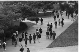
(a)

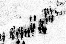
(b)

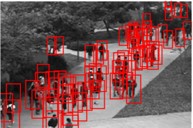
(c)

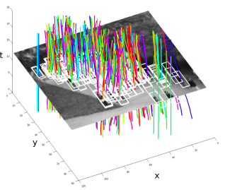
(d)

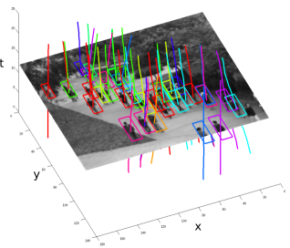
(e)

(f)

Figure 1: Successive stages of the video parsing: (a) Source frame of a video. (b) Foreground probability map that needs to be explained by video parsing. (c) Object candidates found by inverted background detector. (d) Spatio-temporal object hypotheses found by temporal grouping serve as an input to the video parsing. (e) Subset of spatio-temporal object hypotheses that is selected by video parsing to explain the foreground pixels. (f) Normal object prototypes found by video parsing to explain the selected object hypotheses. Best viewed in color.

3 Model for Spatio-temporal Video Parsing

In case of a stationary camera, the foreground/background segregation becomes feasible due to background subtraction. The foreground mask renders it then possible to turn the abnormality detection problem into a task of video parsing. The goal is thus to explain all the foreground of a video using object hypotheses and to explain each hypothesis by an object model learned from the set of normal training videos. The underlying statistical inference problem has to be tackled jointly for all hypotheses, since hypotheses can explain each other away. Abnormalities are then those hypotheses that are required to explain the foreground but which themselves cannot be explained by any prototype from the normal object model.

Foreground segmentation. Scenarios for abnormality detection often involve the analysis of videos from static cameras. Background in such videos is constant or changes slowly over time, hence it can be learned effectively from a video. The resulting background model can then be applied to find all foreground pixels in the video. The final foreground/background segmentation is represented by a binary variable $f_{j}^{t}\in\{0,1\}$ for all pixels $j$ in frame $t$.

Background subtraction assumes that each frame $I^{t}$ of a video can be expressed as the background model $B^{t}$ plus a sparse vector $I^{t}-B^{t}$ whose nonzero elements are the foreground pixels. After stacking successive video frames as columns in a matrix $I=\bigl{[}I^{t-\tau}\ \cdots\ I^{t}\bigr{]}$, we want to find the low-rank background model $B$ such that the sparsity inducing norm of the difference $I-B$ is the smallest possible. Following the approach of Wright et al. [5], we approximate the rank of the matrix $B$ by a nuclear norm $\|\cdot\|_{*}$ and use $\ell_{1}$ as the sparsity inducing norm, so that the background subtraction becomes the following convex optimization problem,

$$B=\operatornamewithlimits{argmin}_{\tilde{B}}\|\tilde{B}\|_{*}+\|I-\tilde{B}\|_{1}.$$ (1)

Now that we calculated the background model $B$, it can be used to find all foreground pixels $j$, $f_{j}^{t}=1$, as those that have a large discrepancy between the observation $I_{j}^{t}$ and the background model $B_{j}^{t}$. The probability that a pixel is foreground $P(f_{j}^{t}=1)$ is obtained by the sigmoid transformation of the difference of pixel’s intensity and background model,

$$P(f_{j}^{t}=1)=2\Bigl{(}1+\exp(-\lambda\|I_{j}^{t}-B_{j}^{t}\|)\Bigr{)}^{-1}-1.$$ (2)

Pixels with foreground probability greater than $0.5$ are considered as foreground, $f_{j}^{t}=1$, and others as background, $f_{j}^{t}=0$.

Shortlist of Object Hypotheses. For parsing the video, we need to specify a list of spatio-temporal object hypotheses that is sufficient for explaining foreground pixels in video. An input to our video parsing algorithm consists of the most suitable object hypotheses for the task of foreground explanation. In Sect. 6 we explain the procedure for creating a shortlist of object hypotheses that has a high recall, i.e. where the majority of true-positive object hypotheses is included in the shortlist. However, as the precision rate of the proposed shortlist is low, there will be many superfluous hypotheses that are then explained away by others during video parsing.

We assume that hypotheses from the shortlist span a time window $\{t-\tau,\dots,t\}$. Each hypothesis $h$ represents a spatio-temporal tube covering locations $l_{h}:=(l_{h}^{t-\tau}\ \dots\ l_{h}^{t})$. This is a trajectory of locations $l_{h}^{t}=(x_{h}^{t}\ y_{h}^{t}\ s_{h}^{t})^{\top}$, which specify the center $(x_{h}^{t},y_{h}^{t})$ and the scale $s_{h}^{t}$ of a candidate object $h$ at time $t$. The scale of an object represents its size relative to the size $(W,H)$ of the object model. The support region of an object hypothesis $h$ at time $t$ is the bounding box of size $(s_{h}^{t}W,\ s_{h}^{t}H)$, and the set of all pixels $j$ that belong to it is denoted by $\mathcal{S}_{h}^{t}$.

The goal of video parsing is then to select a subset from the shortlist of hypotheses that is both necessary and sufficient for explaining the foreground of a test video while, at same time, finding normal object prototypes that explain the hypotheses of the subset (see Fig. 1).

Figure 2: Probabilistic graphical model of the spatio-temporal video parsing. The left plate contains all spatio-temporal hypotheses $h$ with their descriptors $d_{h}$ and locations $l_{h}$. The right plate comprises all pixels $j$ with their foreground labels $f_{j}^{t}\in\{0,1\}$. By video parsing, we infer the set of hypotheses, $o_{h}\in\{0,1\}$, that are necessary for explaining the foreground, and jointly explain the selected hypotheses by the normal object prototypes $m_{h}\in\{1,\dots,K\}$. Finally, for each selected hypothesis $h$ we decide if it is abnormal, $a_{h}\in\{0,1\}$, and also mark foreground pixels that belong to abnormal objects, $a_{j}^{t}\in\{0,1\}$.

Spatio-temporal object descriptor. A spatio-temporal hypothesis $h$ matches its corresponding normal object prototype both in appearance and motion. Thus, we need a spatio-temporal descriptor $d_{h}$ to capture the essence of both appearance and motion of hypothesis $h$. We build a spatio-temporal descriptor $d_{h}:=\bigl{(}d_{h}^{t-\tau}\ \dots\ d_{h}^{t}\bigr{)}^{\top}$ by concatenating frame-wise descriptors $d_{h}^{t}$ calculated at each time $t$. Frame-wise object appearance is represented by the spatial derivatives of pixel’s intensity in the support region $\mathcal{S}_{h}^{t}$ of hypothesis $h$. Analogously, object motion is represented by the temporal derivatives of pixel’s intensity. The appearance and motion representations are combined into frame-wise descriptor,

$$d_{h}^{t}:=\Bigl{(}\frac{\partial I_{j}^{t}}{\partial x},\ \frac{\partial I_{j}^{t}}{\partial y},\ \frac{\partial I_{j}^{t}}{\partial t}\Bigr{)}_{j\in\mathcal{S}_{h}^{t}}.$$ (3)

Since the spatio-temporal descriptor $d_{h}$ is long and redundant, we build its compact representation by applying PCA transformation that projects onto eigen-space such that most of the signal variation is preserved (about $95\%$).

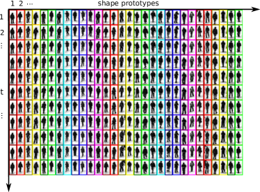
(a)

Figure 3: The normal object model consist of a set of spatio-temporal shape prototypes, each being a sequence that captures the temporal evolution of a particular shape. Prototypes are accompanied by the appearance and motion descriptors.

Activating hypotheses needed for parsing. Not all object hypotheses from the shortlist are needed to explain foreground pixels in video. Video parsing retains only the indispensable hypotheses that cannot be explained away by other hypotheses. Therefore, we use an indicator variable $o_{h}\in\{0,1\}$ for each hypothesis $h$ to designate the hypothesis as active/inactive. To initialize parsing, a discriminative classifier is trained to distinguish background spatio-temporal patterns from anything else. This background classifier computes the probability that hypothesis $h$ is background, $P(o_{h}=0|d_{h})$, which is then inverted to obtain the foreground probability. A hypothesis with high foreground probability can still become inactive if it gets explained away by others during video parsing.

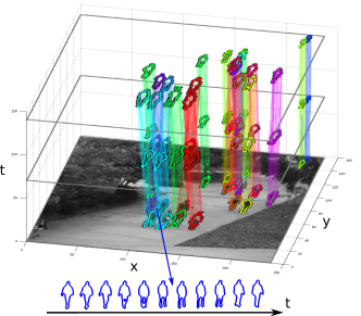
(a)

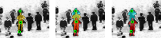
(b)

Figure 4: (a) Spatio-temporal tubes illustrate the hypotheses selected by video parsing. Normal shape contours that explain the hypotheses are shown overlaid. (b) Superfluous hypotheses are eliminated by the statistical inference of explaining away. The idea is the following: Object hypothesis (yellow) is used at the beginning of video parsing to explain the foreground pixel in the middle. Other object hypotheses (red and blue) are introduced later to explain the top and bottom pixels. However, the pixel in the middle is also explained by new hypotheses, so that the original (yellow) hypothesis is not needed anymore and it can be eliminated.

Matching with the object model. Video parsing jointly explains foreground pixels with object hypotheses, and active hypotheses $\{h:o_{h}=1\}$ with normal object prototypes learned from the training data. The object model consists of $K$ normal object prototypes that represent a diversity of normal object’s shape, appearance, and motion. Video parsing then determines for each selected hypothesis $h$ which of the $K$ prototypes best explains it. The prototype that video parsing associates with hypothesis $h$ is indicated by the variable $m_{h}\in\{1,\dots,K\}$. Sect. 5 explains in detail the learning of the normal object prototypes. For the time being, we assume that $K$ normal object prototypes are provided as input to the parsing algorithm.

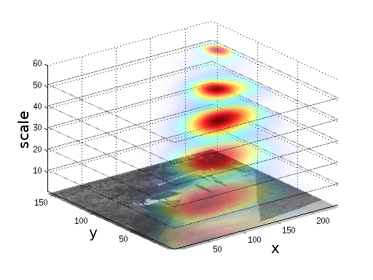
Figure 5: The distribution of locations of normal object prototypes estimated by the Parzen windows at multiple scales (represented as horizontal slices).

For each hypothesis $h$ the best prototype $m_{h}\in\{1,\dots,K\}$ from the learned object model is sought (Fig. 3). For abnormal objects all prototypes will obviously have high matching costs. Consequently, the probability that prototype $m_{h}$ is matched to a hypothesis $h$ in a query video depends on how similar they are in both appearance and motion, $\Delta(d_{h},d_{m_{h}})$. Here, $\Delta$ denotes a function that measures the distance of spatio-temporal descriptors in the corresponding feature space. Given the spatio-temporal descriptor $d_{h}$ of hypothesis $h$, the probability of matching prototype $m_{h}$ with the hypothesis $h$ is the Gibbs distribution,

$$P(m_{h}|d_{h})=\frac{1}{Z(d_{h})}\exp\bigl{(}-\beta\Delta(d_{h},d_{m_{h}})\bigr{)},$$ (4)

where $Z(d_{h})$ is the partition function used to normalize the probability distribution.

Moreover, normal objects typically occupy some location in a scene more often than other, and also tend to move at a certain speed. For example, cars are more likely to drive on roads than on sidewalks, whereas pedestrians are more likely to walk on sidewalks. Consequently, the probability of observing hypothesis $h$ that matches the prototype $m_{h}$ depends on its location $l_{h}^{t}$ and velocity $l_{h}^{t}-l_{h}^{t-1}$,

$$P(l_{h}|m_{h})\propto P_{m_{h}}^{loc}(l_{h}^{t})\cdot P_{m_{h}}^{vel}(l_{h}^{t}-l_{h}^{t-1}).$$ (5)

The normal location and velocity distributions $P_{\bullet}^{loc}$ and $P_{\bullet}^{vel}$ are learned for each of the $K$ object prototypes using the Parzen window density estimator (see Fig. 5).

Therefore, the probability that hypothesis $h$ matches to the normal object prototype $m_{h}$ is

$$P(m_{h}|o_{h},d_{h},l_{h})\propto o_{h}\cdot P(m_{h}|d_{h})\cdot P(l_{h}|m_{h}).$$ (6)

Explaining foreground pixels. Video parsing selects hypotheses, $\{h:o_{h}=1\}$, and finds corresponding normal object prototypes $m_{h}$ to explain the foreground. The foreground probability of a pixel $j$ depends on all hypotheses $h$ that overlap with pixel $j$. Given the support regions $\mathcal{S}_{h}^{t}$ of all hypotheses $h$, $\{h:j\in\mathcal{S}_{h}\}$ is the set of hypotheses that cover the pixel $j$. The probability that pixel $j$ is background is equal to the product of pixel’s background probabilities for each single hypothesis $h$ that contains the pixel $j$. Even if all hypotheses claim that pixel $j$ is background, $P\bigl{(}f_{j}^{t}=1|o_{h},m_{h},l_{h}\bigr{)}=0,\ \forall h$, we still allow it to be foreground with a small foreground probability $P_{0}>0$ . Thus, foreground probability of pixels $j$ given all hypotheses is

$$P(f_{j}^{t} =1|\{o_{h},m_{h},l_{h}\}_{h})=$$

$$1-(1-P_{0})\prod_{h}\Bigl{(}1-P(f_{j}^{t}=1|o_{h},m_{h},l_{h})\Bigr{)}.$$ (7)

The foreground probability given a single hypothesis $h$, $P(f_{j}^{t}=1|o_{h},m_{h},l_{h})$, depends on the shape of the corresponding normal object prototype $m_{h}$. In the training data, the prototype $m_{h}$ covers pixels $j^{\prime}$ with some probability $P_{m_{h}}(f_{j^{\prime}}^{t}=1)$. Thus, the foreground probability of pixel $j$ under hypothesis $h$ is obtained by taking its corresponding object prototype $m_{h}$ and “pasting” the foreground probability of $m_{h}$ at the location of $h$. The model now needs to be brought into the reference frame of $h$ by scaling and translating it, i.e. $l_{j}^{t}=s_{h}^{t}\cdot l_{j^{\prime}}^{t}+(x_{h}^{t}\ y_{h}^{t})^{\top}$. Then the foreground probability of pixel $j$ given $h$ becomes

$$P(f_{j}^{t}=1|o_{h},m_{h},l_{h})=o_{h}\cdot\mathbf{1}[j\in\mathcal{S}_{h}^{t}]$$

$$\cdot\sum_{j^{\prime}}\mathbf{1}[l_{j}^{t}=s_{h}^{t}\cdot l_{j^{\prime}}^{t}+(x_{h}^{t}\ y_{h}^{t})^{\top}]\cdot P_{m_{h}}(f_{j^{\prime}}^{t}=1).$$ (8)

Here $\mathbf{1}[\cdot]$ denotes the indicator function. In Eq. 8 the foreground probability of pixel $j$ is set to zero if hypothesis $h$ is inactive, $o_{h}=0$, or the pixel $j$ does not belong to the support region of hypothesis $h$, $j\notin\mathcal{S}_{h}^{t}$.

4 Inference by Foreground Parsing

The goal is now to estimate which of the hypotheses are actually needed for explaining the foreground and to find a matching normal object prototype for each hypothesis. For abnormal hypotheses Eq. 6 will yield low probabilities. If foreground $f_{j}^{t}=1$ is observed and the pixel is covered by a hypothesis $h$, and no other hypothesis can be found that could explain the presence of the foreground at that pixel, then the probability of activation of hypothesis $h$ increases. This leads to the statistical inference of explaining away. For an observed variable $f_{j}^{t}$ different hypotheses $h$ that share the same pixel $j$ become statistically dependent so that the absence of one hypothesis can dictate the presence of another (see Fig. 4).

4.1 Joint Inference by MAP

Based on the foreground segmentation mask $f_{j}^{t}$ and the shortlist of hypotheses $h$ with spatio-temporal descriptors $d_{h}$ and trajectories $l_{h}$, we need to jointly infer all hidden variables $\{o_{h},m_{h}\}_{h}$ in our graphical model (Fig. 2). Following a maximum a posteriori (MAP) approach yields a set of hypotheses that best explain the foreground and are themselves explained by the normal object prototypes,

$$\{\bar{o}_{h},\bar{m}_{h}\}_{h}=\max_{\{o_{h},m_{h}\}_{h}}P(\{o_{h},m_{h}\}_{h}|\{d_{h},l_{h}\}_{h},\{f_{j}^{t}\}_{j})$$

$$\propto\prod_{j}P\bigl{(}f_{j}^{t}|\{o_{h},m_{h},l_{h}\}_{h}\bigr{)}\prod_{h}P(o_{h}|d_{h})P(m_{h}|o_{h},d_{h},l_{h}).$$ (9)

Instead of explicitly maximizing the posterior probability, we take a negative logarithm of Eq. 4.1 and thereby obtain the energy function $J(\cdot)$ which is then minimized. Furthermore, we decompose the energy function $J(\cdot)$ into two terms, $J_{j}(\cdot)$ covering the explanation of foreground pixels $j$, and $J_{h}(\cdot)$, which involves the explanation of hypotheses $h$ by the normal object prototypes,

$$J(\{o_{h},m_{h}\}_{h}):=\underbrace{-\sum_{j}\log P(f_{j}^{t}|\{o_{h},m_{h},l_{h}\}_{h})}_{=:J_{j}(\{o_{h},m_{h}\}_{h})}$$

$$\underbrace{-\sum_{h}\Bigl{(}\log P(o_{h}|d_{h})+\log P(m_{h}|o_{h},d_{h},l_{h})\Bigr{)}}_{=:J_{h}(\{o_{h},m_{h}\}_{h})}.$$ (10)

To find the MAP solution, we introduce a parsing indicator $z_{h,k}\in\{0,1\}$, that equals one if hypothesis $h$ is active, $o_{h}=1$, and their corresponding normal object prototype is $m_{h}=k$,

$$z_{h,k}:=o_{h}\cdot\mathbf{1}[m_{h}=k],\ \forall h,\ \forall k\in\{1,\dots,K\}.$$ (11)

To keep the notation simple, let the vector $\mathbf{z}_{h}:=(z_{h,1},\dots,z_{h,K})^{\top}$ denote the parsing indicators of hypothesis $h$, and the vector $\mathbf{z}:=\{\mathbf{z}_{h}\}_{h}$ denote the parsing indicators of all hypotheses together. The following lemma now states that the hypotheses explanation $J_{h}(\cdot)$ can be expressed as a linear function of the parsing indicator $\mathbf{z}$.

Lemma 4.1

The hypotheses explanation term $J_{h}(\{o_{h},m_{h}\}_{h})$ in Eq. 10 is a linear function of the parsing indicator $\mathbf{z}$, i.e.

$$J_{h}(\{o_{h},m_{h}\}_{h})=\mathbf{b}^{\top}\mathbf{z}+b_{0},$$ (12)

where the parameter vector $\mathbf{b}=\{b_{h,k}\}_{h,k}$ and scalar $b_{0}$ do not depend on the parsing indicator $\mathbf{z}$. The proof of Lemma 4.1 is given in Appendix A.

To express the foreground explanation term $J_{j}(\cdot)$ as a function of the parsing indicator $\mathbf{z}$, we first define a function $\Phi_{f_{j}^{t}}(\cdot)$ that is parametrized by the foreground value $f_{j}^{t}$ of pixel $j$,

$$\Phi_{f_{j}^{t}}(x):=(1-f_{j}^{t})x-f_{j}^{t}\cdot\log\bigl{(}1-e^{-x}\bigr{)},\ x>0.$$ (13)

The introduced function $\Phi_{f_{j}^{t}}(\cdot)$ is convex as we show in the following lemma.

Lemma 4.2

The function $\Phi_{f_{j}^{t}}(x),\ x>0$ (Eq. 13) is convex for nonnegative values of the parameter $f_{j}^{t}$. The proof of Lemma 4.2 is given in Appendix B.

We also introduce a joint shape prototype vector $\bm{w}:=[\bm{w}_{1}^{\top}\cdots\bm{w}_{K}^{\top}]^{\top}$ that is obtained by concatenating all individual shape prototype vectors $\bm{w}_{k},\ k\in\{1,\dots,K\}$ (c.f. Fig. 3). The component $\bm{w}_{k,j^{\prime}}$ equals the negative logarithm of the background probability of pixel $j^{\prime}$ in the normal shape prototype $\bm{w}_{k}$,

$$\bm{w}_{k,j^{\prime}}=-\log\bigl{(}1-P_{k}(f_{j^{\prime}}^{t}=1)\bigr{)}.$$ (14)

The following lemma establishes a relationship between the foreground explanation term $J_{j}(\mathbf{z})$, the parsing indicator $\mathbf{z}$ and the joint shape prototype vector $\bm{w}$.

Lemma 4.3

The foreground explanation term $J_{j}(\cdot)$ is the sum over all pixels $j$ of convex functions $\Phi_{f_{j}^{t}}(\cdot)$ whose argument is a bilinear function of the parsing indicator $\mathbf{z}$ and the joint shape prototype $\bm{w}$,

$$J_{j}(\mathbf{z}) =\sum_{j}\Phi_{f_{j}^{t}}\bigl{(}\bm{w}^{\top}\mathbf{{C}}_{j}\mathbf{z}+c_{0}\bigr{)}.$$ (15)

The parameter matrices $\mathbf{{C}}_{j}$ and scalar $c_{0}$ do not depend on the parsing indicator $\mathbf{z}$ or joint shape prototype $\bm{w}$. The proof of Lemma 4.3 is given in Appendix C.

In Lemmas 4.3 and 4.1 we expressed the foreground and hypotheses explanation terms $J_{j}(\cdot)$ and $J_{h}(\cdot)$ as convex functions of the parsing indicator $\mathbf{z}$. Therefore, the video parsing objective function $J(\cdot):=J_{j}(\cdot)+J_{h}(\cdot)$ (Eq. 10) is a convex function of the parsing indicator $\mathbf{z}$. To efficiently solve the optimization problem, we relax the parsing indicator $\mathbf{z}$ to the positive simplex, $\mathbf{z}_{h}\succeq 0$ and $\mathbf{1}^{\top}\mathbf{z}_{h}\leq 1,\ \forall h$. The last inequality follows from Eq. 11 and the fact that $o_{h}\leq 1$.

The MAP inference in our video parsing model is thus equivalent to the following constrained convex optimization problem,

$$\operatornamewithlimits{argmin}_{\mathbf{z}}J(\mathbf{z})=\mathbf{b}^{\top}\mathbf{z}+b_{0}+\sum_{j}\Phi_{f_{j}^{t}}\bigl{(}\bm{w}^{\top}\mathbf{{C}}_{j}\mathbf{z}+c_{0}\bigr{)},$$

$$\text{s.t. }\mathbf{z}_{h}\succeq 0\text{ and }\mathbf{1}^{\top}\mathbf{z}_{h}\leq 1,\ \forall h.$$ (16)

After finding the optimal value of the parsing indicator $\mathbf{z}$, we calculate the hypothesis indicator $o_{h}$, and the matching normal object prototype $m_{h}$ of hypothesis $h$, as

$$o_{h} =\sum_{k=1}^{K}z_{h,k},$$ (17)

$$m_{h} =\operatornamewithlimits{argmax}_{k}z_{h,k}.$$ (18)

4.2 Solving the Convex Optimization Problem

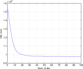
Figure 6: Values of the objective function $J(\mathbf{z})$ (Eq. 16) that are obtained as part of the convex optimization procedure that is used to solve the proposed video parsing problem.

In the previous section, we showed that the joint inference of variables $\{o_{h},m_{h}\}_{h}$ can be achieved by minimizing the MAP objective function $J(\mathbf{z})$ to obtain the parsing indicator $\mathbf{z}$ (Eq. 16), that belongs to the Cartesian product $\mathbf{{Z}}=\mathbf{{Z}}_{h}\times\dots\times\mathbf{{Z}}_{h}$ of positive simplexes,

$$\mathbf{{Z}}_{h}=\{\mathbf{z}_{h}:\mathbf{z}_{h}\succeq 0\text{ and }\mathbf{1}^{\top}\mathbf{z}_{h}\leq 1\}.$$ (19)

The function $J(\mathbf{z})$ is convex, smooth and bounded on the set $\mathbf{{Z}}$. The projected gradient method [40],

$$\mathbf{z}^{n+1}=\text{Proj}_{\mathbf{{Z}}}(\mathbf{z}^{n}-\alpha_{n}\nabla_{\mathbf{z}}J(\mathbf{z}^{n})),$$ (20)

converges to the global optimum of the convex optimization problem in Eq. 16, because of the Lipschitz-continuity of the first derivative of function $\Phi_{f_{j}^{t}}(\cdot)$ as stated in the following lemma.

Lemma 4.4

The first derivative of the function $\Phi_{f_{j}^{t}}(x)$ is $\rho$-Lipschitz continuous in argument $x\geq c_{0}$, i.e. there is a constant $\rho$ such that

$$\bigl{|}\Phi_{f_{j}^{t}}^{\prime}(x_{1})-\Phi_{f_{j}^{t}}^{\prime}(x_{2})\bigr{|}\leq\rho|x_{1}-x_{2}|,\ \forall x_{1},x_{2}\geq c_{0}.$$ (21)

The proof of Lemma 4.4 is given in Appendix D.

The projection $\text{Proj}_{\mathbf{{Z}}}(\cdot)$ requires each $\mathbf{z}_{h}$ to be projected onto the positive simplex $\mathbf{{Z}}_{h}$. The projection onto the positive simplex is calculated by applying the method of Duchi et al. [41]. The projected gradient method finds the solution of the video parsing after only few tens of iterations (Fig. 6).

4.3 From Inference to Abnormalities

Video parsing analyses the foreground in a video and identifies objects that have atypical appearance or behave suspiciously, to label these as abnormal. Abnormalities can also be localized on the level of pixels, where it leads to a segmentation of regions in the video that contain irregular spatio-temporal patterns. Subsequently, we see how both the object-level and pixel-level abnormalities can be detected in video, based on the inference results of our video parsing approach.

Object-level abnormalities. A hypothesis $h$ is an abnormal object, $a_{h}=1$, if it is indispensable for explaining the foreground, $\bar{o}_{h}=1$, but it does not have a matching normal object prototype, i.e., the best estimate $\bar{m}_{h}$ of a matching prototype is unlikely to explain the hypothesis (cf. Eq. 6),

$$P(a_{h}=1|o_{h}=\bar{o}_{h},m_{h}=\bar{m}_{h})$$

$$\propto\bar{o}_{h}P(o_{h}=1|d_{h})P(m_{h}\neq\bar{m}_{h}|o_{h}=\bar{o}_{h},d_{h},l_{h})$$ (22)

$$\propto\bar{o}_{h}P(o_{h}=1|d_{h})\Bigl{(}1-P(m_{h}=\bar{m}_{h}|d_{h})P(l_{h}|m_{h}=\bar{m}_{h})\Bigr{)}.$$ (23)

Pixel-level abnormalities. Similarly, a pixel $j$ is part of an abnormal object, $a_{j}^{t}=1$, if it is in the foreground, $f_{j}^{t}=1$, and at least one of the hypotheses that extend over this pixel, $\{h:j\in\mathcal{S}_{h}^{t}\}$, is abnormal,

$$P(a_{j}^{t}=1|f_{j}^{t},\{a_{h}\}_{h:j\in\mathcal{S}_{h}^{t}})$$

$$\propto f_{j}^{t}\cdot P(f_{j}^{t}=1)\cdot\max_{h:j\in\mathcal{S}_{h}^{t}}P(a_{h}=1|o_{h},m_{h}).$$ (24)

5 Learning an Object Model for Video Parsing

Parsing query videos for abnormality detection requires an object model. We use training videos that contain a large number of normal object samples but no abnormalities to train the normal object model that consists of prototypes representing the normal object shape, appearance, and motion. As ground truth locations of objects in the training videos are not provided, we infer them by video parsing. However, for video parsing we need to know the normal object prototypes. A standard approach for solving such a problem of mutual dependencies is expectation-maximization (EM) [42]. Given an initial estimate of the normal object prototypes, we use them to parse the training videos, i.e. discover hypotheses that best explain the foreground and are matched to the object prototypes (E-step). Thereafter, we update the object prototypes using the matched hypotheses (M-step). We find the object model by iterating the EM steps until convergence.

The goal of learning is to estimate the normal object shape prototypes $\{\bm{w}_{k}\}_{k}$ (Eq. 14) and their corresponding spatio-temporal descriptors $\{d_{k}\}_{k}$, $k\in\{1,\dots,K\}$. The objective function for learning is the same as for the inference (Eq. 16), except that it is now minimized jointly in terms of shape prototypes $\{\bm{w}_{k}\}_{k}$, their spatio-temporal descriptors $\{d_{k}\}_{k}$, as well as the parsing indicator $\mathbf{z}$ (Eq. 11),

$$\operatornamewithlimits{argmin}_{\{d_{k},\bm{w}_{k}\}_{k},\mathbf{z}}J(\mathbf{z},\{d_{k},\bm{w}_{k}\}_{k})=J_{h}(\mathbf{z},\{d_{k}\}_{k})+J_{j}(\mathbf{z},\{\bm{w}_{k}\}_{k}),$$

$$\text{ s.t. }\bm{w}_{k}\succeq 0,\ \forall k,\ \mathbf{z}_{h}\succeq 0\text{ and }\mathbf{1}^{\top}\mathbf{z}_{h}\leq 1,\ \forall h.$$ (25)

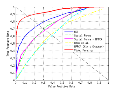
Figure 7: Frame-wise abnormality labeling on the UCSD ped1 dataset. Performance measures AUC and EER given in Tab. I are calculated from the ROC curves.

The hypotheses explanation term $J_{h}(\cdot)$ is a function of the parsing indicator $\mathbf{z}$ and the spatio-temporal descriptors $\{d_{k}\}_{k}$,

$$J_{h}(\mathbf{z},\{d_{k}\}_{k})=\beta\sum_{h}\sum_{k}z_{h,k}\Delta(d_{h},d_{k})+\tilde{\mathbf{b}}^{\top}\mathbf{z}+b_{0},$$ (26)

where the parameters $\tilde{\mathbf{b}}$ and $b_{0}$ do not depend on the parsing indicator $\mathbf{z}$ or the spatio-temporal descriptors $\{d_{k}\}_{k}$ (see the proof of Lemma 4.1 in Appendix A).

From Eq. 15 we see that the foreground explanation term $J_{j}(\cdot)$ depends in a convex way on both the parsing indicator $\mathbf{z}$ and the joint shape prototype vector $\bm{w}$.

Procedure for the object prototype learning. We now explain the EM algorithm used for solving the optimization problem of Eq. 25:

E-step. Given the object prototypes, we parse the training videos to infer the parsing indicator $\mathbf{z}$ (Eq. 16) that yields the hypothesis indicator $o_{h}$ for each hypothesis $h$, and its corresponding normal object prototype $m_{h}$ (Eq. 17 and 18).

M-step. We estimate the shape prototypes $\{\bm{w}_{k}\}_{k}$ and their spatio-temporal descriptors $\{d_{k}\}_{k}$ from the results of video parsing. As hypotheses overlap in training videos, the corresponding shape prototypes become mutually dependent and thus need to be learned jointly. We estimate the joint shape prototype vector $\bm{w}$ by the following convex optimization,

$$\bm{w}=\operatornamewithlimits{argmin}_{\tilde{\bm{w}}\succeq 0}J_{j}(\mathbf{z},\tilde{\bm{w}})=\sum_{j}\Phi_{f_{j}^{t}}(\tilde{\bm{w}}^{\top}\mathbf{{C}}_{j}\mathbf{z}+c_{0}).$$ (27)

The convex optimization problem of Eq. 27 can be solved efficiently by the projected gradient method that we used for solving the MAP inference problem (Eq. 20),

$$\bm{w}^{n+1}=\text{Proj}_{\mathbb{R}_{+}^{|w|}}(\bm{w}^{n}-\alpha_{n}\nabla_{\bm{w}}J_{j}(\mathbf{z},\bm{w}^{n})).$$ (28)

The spatio-temporal descriptors $\{d_{k}\}_{k},\ k\in\{1,\dots,K\}$ are estimated separately for each normal object prototype,

$$d_{k}=\operatornamewithlimits{argmin}_{\tilde{d}_{k}}\sum_{h}z_{h,k}\Delta(d_{h},\tilde{d}_{k}).$$ (29)

In case of a squared Euclidean distance function, $\Delta(d_{h},d_{k})=\|d_{h}-d_{k}\|^{2}$, there is a closed-form solution for $d_{k}$, given as an average of spatio-temporal descriptors $d_{h}$ of those hypotheses that are matched to prototype $k$ by video parsing,

$$d_{k}=\frac{\sum_{h}z_{h,k}d_{h}}{\sum_{h}z_{h,k}}.$$ (30)

The EM algorithm assumes uniform location and velocity distributions (Eq. 5) for normal object prototypes. However, after the EM algorithm is converged, we estimate the prototype’s location and velocity distributions from matched object hypotheses by the non-parametric Parzen windows.

TABLE I: Performance measures on the UCSD ped1 dataset

	frame-wise		pixel-wise partial		pixel-wise full
	AUC ($\%$)	EER ($\%$)	AUC ($\%$)	RD ($\%$)	AUC ($\%$)	RD ($\%$)
Social force [43]	67.5	31	19.7	21	-	-
MPPCA [21]	59	40	20.5	18	-	-
Social force + MPPCA	67	32	21.3	28	-	-
Adam [20]	65	38	13.3	24	-	-
Sparse [29]	86	19	46.1	46	-	-
LSA [30]	92.7	16	-	-	-	-
SCL [31]	91.8	15	63.8	59.1	-	-
MDT [1]	81.8	25	44.1	45	-	-
HMDT CRF [26]	-	17.8	66.2	64.8	82.7	74.5
SVP [39]	91	18	75.6	68	83.6	77
STVP	93.9	12.9	80.3	75.2	84.2	79.5

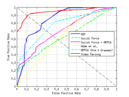
(a)

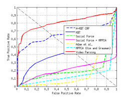
(b)

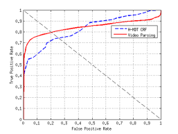
(c)

Figure 8: (a) Frame-wise abnormality labeling for the UCSD ped2 dataset. (b) Pixel-wise abnormality prediction evaluated by the partially annotated UCSD ped1 dataset. (c) Pixel-wise abnormality prediction that is evaluated using the full annotation of the complete UCSD ped1 dataset that we have assembled. In all of these cases our approach significantly improves upon the state-of-the-art, which can also be seen from the corresponding AUC and RD values provided in Tab. I and II.

$\begin{array}[]{cccc}\includegraphics[width=95.39693pt]{./figures/ped1_001_hi_110.png}&\includegraphics[width=95.39693pt]{./figures/ped1_001_mi_110.png}&\framebox{\includegraphics[width=95.39693pt]{./figures/ped1_001_aj_110.png}}&\includegraphics[width=95.39693pt]{./figures/ped1_001_nuno_110.png}\\ \includegraphics[width=95.39693pt]{./figures/ped1_031_hi_104a.png}&\includegraphics[width=95.39693pt]{./figures/ped1_031_mi_104.png}&\framebox{\includegraphics[width=95.39693pt]{./figures/ped1_031_aj_104.png}}&\includegraphics[width=95.39693pt]{./figures/ped1_031_nuno_104.png}\\ \includegraphics[width=95.39693pt]{./figures/ped1_018_hi_098.png}&\includegraphics[width=95.39693pt]{./figures/ped1_018_mi_098.png}&\framebox{\includegraphics[width=95.39693pt]{./figures/ped1_018_aj_098.png}}&\includegraphics[width=95.39693pt]{./figures/ped1_018_nuno_098.png}\\ \includegraphics[width=95.39693pt]{./figures/ped1_019_hi_112a.png}&\includegraphics[width=95.39693pt]{./figures/ped1_019_mi_112.png}&\framebox{\includegraphics[width=95.39693pt]{./figures/ped1_019_aj_112.png}}&\includegraphics[width=95.39693pt]{./figures/ped1_019_nuno_112.png}\end{array}$

Figure 9: Rows show results on different frames of the UCSD ped1 benchmark. Column i) the initialization of the video parsing by a shortlist of object hypotheses, column ii) hypotheses selected by video parsing with the best matching shape prototype colored according to abnormality probability $P(a_{h}^{t}=1)$, column iii) foreground pixel abnormality probabilities $P(a_{j}^{t}=1)$, column iv) results by the H-MDT CRF approach [26]. Best viewed in color.

Initialization. To start the EM algorithm, we need an initial estimate of the normal object model. After background subtraction, some foreground segments correspond to isolated normal objects that can be used to initialize our object prototypes. However, foreground/background segmentation produces also many foreground segments which correspond to interacting objects (doublets, triplets etc.). These segments are more complex and can be analyzed only by video parsing. Consequently, we need to infer which of the training foreground segments correspond to isolated normal objects and estimate object prototypes based upon them. We observe that isolated normal objects create compact clusters in the feature space. On the other hand, segments that are mixtures of two or more objects are diverse and spread out in the feature space. To detect isolated normal objects, we cluster all the foreground segments and then select compact clusters in the feature space that correspond to isolated objects. We use Ward’s method for agglomerative clustering to minimize the variance of clusters. Normal object prototypes are then computed as the centers of compact clusters.

6 Creating Initial Object Hypotheses

To initialize video parsing, we need a shortlist of spatio-temporal object hypotheses $h$ (Sect. 3). A spatio-temporal hypothesis $h$ consists of a sequence of object candidates in individual frames that are linked temporally. In this section we explain a method for producing per-frame object candidates and group them temporally based on their motion to obtain the shortlist of Sect. 3. Thereafter, we explain how to fill-in per-frame candidates that were missed during temporal grouping.

Temporal grouping of per-frame object candidates. To detect per-frame object candidates, we apply an inverted background detector that is trained to distinguish background patterns from everything else. The inverted background detector is trained on background and normal foreground segments obtained from training videos by background subtraction. The discriminative appearance-based classifier retains in each frame the object candidates that are least likely to be background. The standard non-maximum suppression (NMS) then removes some of the candidates based on the overlap criteria. The discriminative classifier is trained using a linear SVM [44] with frame-wise descriptor of Eq. 3 extracted from background/foreground segments of training videos.

We then employ agglomerative clustering to perform a temporal grouping of candidates. This yields spatio-temporal hypotheses $h$, which are sequences of per-frame candidates. As usual, the clustering starts with singleton clusters (each candidate being a cluster). Then, in each round of the recursive clustering, those groups of per-frame object candidates which are most similar based on their motion and which do not share the same frames are grouped. The motion of a candidate is represented by the set of trajectories obtained by tracking the edge points inside the support region of a candidate. For tracking the feature points we use optical flow vectors that are previously computed by the method of [45]. We now define similarity of two object candidates as the ratio of the number of feature point trajectories that are shared by two candidates over the total number of trajectories in two candidates. As the result of temporal grouping, we obtain a shortlist of spatio-temporal hypotheses $h$.

Filling-in missing candidates by Kalman filter. The inverted background detector used for producing object candidates in each frame typically has a number of missed detections. These are the frames in which none of the object candidates is associated with a hypothesis $h$. We fill-in the missed object detections with the contextual help of other per-frame candidates that belong to the same hypothesis $h$. Therefore, the location of a missed object candidate $l_{h}^{t}$ at time $t$ is estimated from the available object candidate locations at times $\{t_{1},t_{2},\dots\}$ by a non-causal Kalman filter.

The shortlist of object hypotheses established by temporal grouping has a high recall at the cost of low precision. By maximizing the recall, the shortlist includes all relevant hypotheses, while still maintaining a reasonable total number thereof (about one hundred). Since hypotheses are created by bottom-up grouping, there will, however, be many spurious hypotheses that can only be eliminated by video parsing.

7 Experimental Evaluation

We use three standard state-of-the-art benchmark sets for evaluating our video parsing approach and comparing its performance to the other state-of-the-art methods. We first analyze the detection results of our approach on the UCSD benchmark sets ped1 and ped2, then we present additional results on the UMN benchmark set. We apply the standard evaluation protocol of the datasets.

7.1 Evaluation on the UCSD Anomaly Datasets

7.1.1 Datasets Description

We use the challenging UCSD anomaly datasets ped1 and ped2, that were recently proposed by Mahadevan et al. [1] for measuring the performance of abnormality detection algorithms. Both datasets consist of videos recorded in crowded walkway scenes that also feature lots of challenging abnormal instances which are objects with unusual appearance or behavior. The UCSD ped1 set contains $34$ training and $36$ test videos that are all $200$ frames long. Due to the low resolution of ped1 videos, the pedestrians who walk towards and away from the camera are only $10-25$ pixels high. In the UCSD ped2 dataset there are $16$ training and $12$ test videos that have a variable length (at most $180$ frames). Pedestrians in these videos are about $30$ pixels high. Videos from both benchmark sets are very crowded, so that object heavily occlude one another.

Abnormalities in the UCSD datasets are not staged but occur naturally in the scene and can be grouped into: i) objects that do not fit to the context of the scene, such as a car on a crowded walkway, or ii) objects that look normal but behave in unusual way, such as people that cycle or skateboard across the walkway or walk in the lawn. Abnormalities from the UCSD benchmark sets include also carts and wheelchairs. We emphasize that the training videos consist only of normal objects and actions, so that a model for abnormalities cannot be learned from it.

7.1.2 Evaluation Protocol

We use the standard protocol for evaluating abnormality detection results that was proposed by Mahadevan et al. [1]. The protocol consists of frame-wise and pixel-wise criteria. The frame-wise criterion labels a frame as abnormal if it contains at least one abnormal object detection. The localization accuracy of detected abnormalities is verified by the pixel-wise criterion that is more rigorous than the frame-wise criterion, since the detected abnormalities are compared to a pixel-level ground-truth mask. The pixel-wise criterion requires that at least $40\%$ of all ground-truth abnormal pixels to be marked as abnormal in order to count a frame as true positive. By calculating the true positive rate (TPR) and false positive rate (FPR) at different detection thresholds we obtain the receiver operating characteristic (ROC).

Frame-wise and pixel-wise criteria use the area under the curve (AUC) as a performance measure calculated directly from the corresponding ROC curve. For the frame-wise criterion we calculate also the equal error rate (EER) as a value obtained when the false positive and false negative rates are equal. For pixel-wise criterion we compute the rate of detection (RD), that is equal to $1-$EER. The pixel-wise criterion is applied on the partially labeled UCSD ped1 dataset originally provided with the pixel-wise ground-truth annotation. Moreover, we also provide complete pixel-wise ground-truth annotations for the full datasets and evaluate thereon.

TABLE II: Performance measures on the UCSD ped2 dataset

	frame-wise		pixel-wise
	AUC ($\%$)	EER ($\%$)	AUC ($\%$)	RD ($\%$)
Social force [43]	63	42	-	-
MPPCA [21]	77	30	-	-
Social force + MPPCA	71	36	-	-
Adam [20]	63	42	-	-
MDT [1]	85	25	-	-
H-MDT CRF [26]	-	18.5	-	70.1
SVP [39]	92	14	-	-
STVP	94.6	10.6	81.1	78.8

7.1.3 The Results of Evaluation

Fig. 9 compares the abnormality localization of our video parsing to the H-MDT CRF method [26] on UCSD ped1 test videos. The first row shows a person riding a bike in a group of walking persons. In the second row there are three abnormalities in the scene: a person riding a bike, and two persons running along the walkway. The third row shows a person skateboarding along the walkway, and the fourth row shows an unusual object (car) in the scene. The columns show: (i) initial hypotheses of video parsing, (ii) hypotheses selected by video parsing, (iii) abnormality localization results of video parsing, (iv) abnormality localization results of H-MDT CRF method [26]. Due to our learned normal shape model used for explaining the foreground, we achieve better localization of the abnormalities in videos.

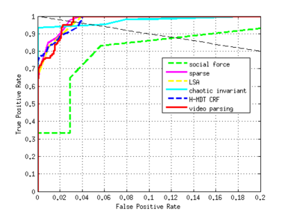
(a)

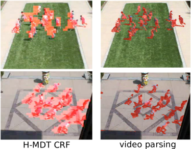
(b)

Figure 10: Abnormality detection on the UMN dataset. (a) ROC curves for frame-wise labeling. (b) Detection results of the H-MDT CRF [26] (left column) and video parsing (right column). Our approach exhibits competitive performance as can also be seen from the corresponding AUC and EER statistics in Tab. 10.

TABLE III: Performance measures on
the UMN dataset

method	AUC ($\%$)	EER ($\%$)
chaotic invariants [46]	99.4	5.3
social force [43]	94.9	12.6
LSA [30]	99.5	3.4
H-MDT CRF [26]	99.5	3.7
Sparse [29] (scene1)	99.5	-
Sparse [29] (scene2)	97.5	-
Sparse [29] (scene3)	96.4	-
STVP (scene1)	99.5	3.2
STVP (scene2)	97.5	6.2
STVP (scene3)	99.9	1.5

In Fig. 12 we show more examples of the video parsing on UCSD ped1 test videos. Row $1$ shows two persons skateboarding and cycling on a very crowded walkway, row $2$ a skateboarder in a group of pedestrians, and row $3$ two cyclists and a person walking across the walkway. By comparing the first two columns one can see that most hypotheses from the shortlist are discarded by video parsing because they get statistically explained away.

We also compare quantitatively our video parsing approach to the state-of-the-art methods on the challenging UCSD ped1 and ped2 benchmarks [1]. The methods used in our comparison are the mixture of dynamic textures (MDT) [1], H-MDT CRF [26], social force model (SF) [43], mixture of optical flow (MPPCA) [21], optical flow method (Adam et al.) [20], SF+MPPCA [1], sparse reconstruction (Sparse), local statistical aggregates (LSA) [30], and sparse combination learning (SCL) [31]. Our previous approach [39] which parses video frames individually, one after another, is denoted as sequential video parsing (SVP). We denote by STVP the full spatio-temporal video parsing proposed in this paper.

Figure 11: Analysis of the false positive instances generated by our video parsing on the UCSD ped1 dataset. Instances are sorted in the decreasing order of their abnormality score.

Our study shows that video parsing outperforms all other methods in experiments on both UCSD ped1 and ped2 datasets. Fig. 7 shows ROC curves for the frame-wise labeling of the UCSD ped1 set. Tab. I gives the performance measures for the ped1 dataset. We see that the inclusion of the temporal component and the improved inference enables spatio-temporal video parsing to improve upon our previous sequential video parsing by $2.9\%$ in AUC and $5.1\%$ in EER. From Tab. I we also see that our approach improves upon recently proposed powerful methods such as LSA [30] ($1.2\%$ gain in AUC and $3.1\%$ in EER) as well as SCL [31] ($2.1\%$ gain in AUC and EER). All ROC plots for the pixel-wise labeling on ped1 are shown in Fig. 8 b) and c). For the partial pixel-wise labeling of ped1, the spatio-temporal video parsing achieves an improvement of $4.7\%$ AUC and $7.2\%$ RD over the sequential video parsing. We outperform the closest competitor (HDMT CRT [26]) by $14.1\%$ in AUC and $10.4\%$ in RD. For the full pixel-wise labeling of ped1, we achieve an improvement of $2.5\%$ in RD over the sequential video parsing. The competing HMDT CRF [26] method we outperform in this case by $1.5\%$ in AUC and $5.0\%$ in RD.

The ROC curves for the frame-wise labeling of UCSD ped2 are given in Fig. 8 a). The numerical results are given in Tab. II. We observe an improvement in performance of spatio-temporal parsing over sequential parsing by $2.6\%$ in AUC and $3.4\%$ in EER. The best method so far, MHDT CRF [26], we improve upon by $6.9\%$ in EER. For the pixel-wise labeling of ped2 dataset, we outperform the competing HMDT CRF method by $8.7\%$ RD (AUC values for HMDT CRF are not provided in [26]). Overall we see that our spatio-temporal reasoning and the convex optimization based inference yield a significant improvement over the state-of-the-art.

Due to temporal grouping of per-frame object candidates (Sect. 6), spatio-temporal video parsing requires significantly less hypotheses (only about a hundred for the whole spatio-temporal domain) than sequential video parsing [39], which needs the same number of hypotheses for representing single frames. Since there remain fewer hypotheses to process, spatio-temporal video parsing takes less time to execute than sequential video parsing. Our non-optimized Matlab implementation on a Dual-Core 2.7GHz CPU runs at about $1$ fps, whereas our previous sequential video parsing took $5$-$10$ secs per frame. This is on par with recent H-MDT CRF [26] and Sparse [30] methods, with a notable exception of extremely fast SCL method [31].

$\begin{array}[]{cccc}\includegraphics[width=91.0631pt]{./figures/ped1_002_hi_116a.png}&\includegraphics[width=91.0631pt]{./figures/ped1_002_oi_116.png}&\includegraphics[width=91.0631pt]{./figures/ped1_002_mi_116.png}&\framebox{\includegraphics[width=91.0631pt]{./figures/ped1_002_aj_116.png}}\\ \includegraphics[width=91.0631pt]{./figures/ped1_034_hi_089.png}&\includegraphics[width=91.0631pt]{./figures/ped1_034_oi_089.png}&\includegraphics[width=91.0631pt]{./figures/ped1_034_mi_089.png}&\framebox{\includegraphics[width=91.0631pt]{./figures/ped1_034_aj_089.png}}\\ \includegraphics[width=91.0631pt]{./figures/ped1_033_hi_055a.png}&\includegraphics[width=91.0631pt]{./figures/ped1_033_oi_055.png}&\includegraphics[width=91.0631pt]{./figures/ped1_033_mi_055.png}&\framebox{\includegraphics[width=91.0631pt]{./figures/ped1_033_aj_055.png}}\end{array}$

Figure 12: Additional results of video parsing on the UCSD ped1 dataset. Rows correspond to different examples. The first, third and fourth column correspond to the first three columns of Fig. 9. The second column shows hypotheses that are selected from the shortlist by video parsing. Other hypotheses are discarded by explaining away using the selected hypotheses. Best viewed in color.

7.1.4 Analysis of False Detections

To get a full understanding of the detection performance of proposed video parsing, we analyze the false detections on the UCSD ped1 dataset. In Fig. 11 we see the first $225$ false detections sorted in the decreasing order of their probability of abnormality. We observe several reasons for false detections: i) In many cases, false detections appear as a result of artifacts in the foreground segmentation. In such cases, wrongly segmented pixels cannot be explained by the learned shape model and thus they are classified as abnormal. ii) Large variability of the normal human gait can sometimes be interpreted in video parsing as abnormal (e.g. running vs. fast walking). iii) Seldom errors in the provided video annotation cause that correctly detected abnormalities are sometimes considered as false (e.g. cars or running persons in Fig. 11). iv) When the true-positive hypothesis is missing from the shortlist due to a non-maximal recall, video parser can select an incorrect hypothesis as a next best fit.

7.2 Evaluation on the UMN Anomaly dataset

We additionally evaluate our video parsing on the UMN dataset that is widely used for benchmarking abnormality detection. The UMN dataset consists of three scenes in which periods of normal activity are followed by periods of emergency that are staged by people in the scene. In normal cases people are walking around alone or in groups. However, in emergency cases people start in panic to run away. For each scene several normal and abnormal events are happening one after another. In scene one, two and three there are two, six and three abnormal events, respectively. The dataset does not provide pixel-wise ground-truth abnormality maps, so we follow the standard protocol for this dataset and evaluate the detection results only in a frame-wise manner. Fig. 10 a) shows ROC curves for the frame-wise labeling. The performance measures AUC and EER are given in Tab. 10. For scene one, our performance is on par with the best competing methods in terms of AUC ($99.5\%$) and EER($3.2\%$). For scene two we achieve $97.5\%$ AUC that is equal to the best performing method (Sparse [29]). For the scene three we achieve $99.9\%$ AUC that improves upon the best competitor (Sparse [29]) by $3.5\%$. A qualitative comparison of our method to HMDT CRF [26] on two frames is shown in Fig. 10 b). We see that our method achieves best localization of abnormalities that is consistent with findings from earlier experiments on UCSD ped1 and ped2.

8 Conclusion

In this paper we have framed abnormality detection as spatio-temporal video parsing to circumvent the ill-posed problem of directly searching for individual abnormal local image regions. We detect abnormalities by searching for a set of spatio-temporal object hypotheses that jointly explain the video foreground and which are themselves explained by normal training samples. In video parsing we do not independently detect individual hypotheses, but their joint layout that collectively describes the objects in the scene. We use MAP inference in a graphical model to effectively localize abnormalities in video and solve it as a convex optimization problem. We have evaluated our approach on several challenging datasets, which show that video parsing advances the state-of-the-art both in terms of abnormality classification and localization.

Appendix A Proof of Lemma 4.1

Proof:

The hypotheses explanation $J_{h}(\{o_{h},m_{h}\}_{h})$ (Eq. 10) can be written as follows,

$$J_{h}(\{o_{h},m_{h}\}_{h})=\sum_{h}\Bigl{\{}-(1-o_{h})\log P(o_{h}=0|d_{h})$$

$$-o_{h}\log P(o_{h}=1|d_{h})+o_{h}\cdot\log Z(d_{h})$$

$$+\sum_{k=1}^{M}\underbrace{o_{h}\cdot\mathbf{1}[m_{h}=k]}_{=z_{h,k}}\cdot\Bigl{(}\beta\Delta(d_{h},d_{k})$$

$$-\log P_{k}^{loc}(l_{h}^{t})-\log P_{k}^{vel}\bigl{(}l_{h}^{t}-l_{h}^{t-1}\bigr{)}\Bigr{)}\Bigr{\}}.$$

By replacing $o_{h}$ with the sum from Eq. 17, we see that the hypotheses explanation term $J_{h}(\{o_{h},m_{h}\}_{h})$ can be expressed as a linear function of the parsing indicator $\mathbf{z}$,

$$J_{h}(\mathbf{z})=\mathbf{b}^{\top}\mathbf{z}+b_{0},$$

where the parameter vector $\mathbf{b}=\{b_{h,k}\}_{h,k}$ and scalar $b_{0}$ are defined in the following way,

$$b_{h,k} =-\log P(o_{h}=1|d_{h})+\log P(o_{h}=0|d_{h})$$

$$+\log Z(d_{h})+\beta\Delta(d_{h},d_{k})-\log P_{k}^{loc}(l_{h})$$

$$-\log P_{k}^{vel}\bigl{(}l_{h}^{t}-l_{h}^{t-1})$$

$$b_{0} =-\sum_{h}\log P(o_{h}=0|d_{h}),$$

and they do not depend on the parsing indicator $\mathbf{z}$. ∎

Appendix B Proof of Lemma 4.2

Proof:

The second derivative of the function $\Phi_{f_{j}^{t}}(x),\ x>0$ is given as follows,

$$\Phi_{f_{j}^{t}}^{\prime\prime}(x) =f_{j}^{t}\cdot\frac{e^{-x}}{(1-e^{-x})^{2}}.$$

We see that the second derivative is positive, $\Phi_{f_{j}^{t}}^{\prime\prime}(x)>0$, if the parameter $f_{j}^{t}$ is positive, $f_{j}^{t}>0$, so in this case the function $\Phi_{f_{j}^{t}}(x)$ is strictly convex. If the parameter $f_{j}^{t}$ equals zero, $f_{j}^{t}=0$, the function $\Phi_{f_{j}^{t}}(x)$ is linear, $\Phi_{f_{j}^{t}}(x)=x$, and therefore convex as well. ∎

Appendix C Proof of Lemma 4.3

Proof:

The foreground explanation $J_{j}(\{o_{h},m_{h}\}_{h})$ depends on all hypotheses that cover pixel $j$,

$$J_{j} (\{o_{h},m_{h}\}_{h})=$$

$$\sum_{j}\Bigl{\{}-(1-f_{j}^{t})\log P(f_{j}^{t}=0|\{o_{h},m_{h},l_{h}\}_{h})$$

$$-f_{j}^{t}\cdot\log\bigl{(}1-P(f_{j}^{t}=0|\{o_{h},m_{h},l_{h}\}_{h})\bigr{)}\Bigr{\}}$$

$$=\sum_{j}\Phi_{f_{j}^{t}}\bigl{(}-\log P(f_{j}^{t}=0|\{o_{h},m_{h},l_{h}\}_{h})\bigr{)}.$$

The argument of the function $\Phi_{f_{j}^{t}}(\cdot)$ in the last equation is bilinear in the parsing indicator $\mathbf{z}$ (Eq. 11) and the joint shape prototype vector $\bm{w}$ (Eq. 14),

$$-\log P(f_{j}^{t}=0|\{o_{h},m_{h},l_{h}\}_{h})$$

$$=-\log(1-P_{0})-\sum_{h}\log\bigl{(}1-P(f_{j}^{t}=1|o_{h},m_{h},l_{h})\bigr{)}$$

$$=-\log(1-P_{0})-\sum_{h}\sum_{k}\underbrace{o_{h}\cdot\mathbf{1}[m_{h}=k]}_{=z_{h,k}}\cdot\mathbf{1}[j\in\mathcal{S}_{h}^{t}]$$

$$\cdot\sum_{j^{\prime}}\mathbf{1}[l_{j}^{t}=s_{h}^{t}\cdot l_{j^{\prime}}^{t}+(x_{h}^{t}\ y_{h}^{t})^{\top}]\cdot\underbrace{\log P_{k}(f_{j^{\prime}}^{t}=0)}_{=:-\bm{w}_{k,j^{\prime}}}$$

$$=\bm{w}^{\top}\mathbf{{C}}_{j}\mathbf{z}+c_{0},$$

where $\mathbf{{C}}_{j}$ is a sparse matrix with following elements,

$$\mathbf{{C}}_{j}(k,j^{\prime};h,k)=\mathbf{1}[j\in\mathcal{S}_{h}^{t}]\cdot\mathbf{1}[l_{j}^{t}=s_{h}^{t}\cdot l_{j^{\prime}}^{t}+(x_{h}^{t}\ y_{h}^{t})^{\top}],$$

and the scalar $c_{0}$ has the value $c_{0}=-\log(1-P_{0})$.

Thus, the foreground explanation term $J_{j}(\{o_{h},m_{h}\}_{h})$ can be written as

$$J_{j}(\mathbf{z},\bm{w}) =\sum_{j}\Phi_{f_{j}^{t}}\Bigl{(}\bm{w}^{\top}\mathbf{{C}}_{j}\mathbf{z}+c_{0}\Bigr{)}.$$

∎

Appendix D Proof of Lemma 4.4

Proof:

The expression for the first derivative of the function $\Phi_{f_{j}^{t}}(x)$ is

$$\Phi_{f_{j}^{t}}^{\prime}(x) =1-f_{j}^{t}\cdot\frac{1}{1-e^{-x}},$$

The absolute difference of the first derivative of function $\Phi_{f_{j}^{t}}(x)$ evaluated in points $x_{1},x_{2}\geq c_{0}=-\log(1-P_{0})$ is upper bounded in the following way,

$$\bigl{|}\Phi_{f_{j}^{t}}^{\prime}(x_{1})-\Phi_{f_{j}^{t}}^{\prime}(x_{2})\bigr{|}=f_{j}^{t}\cdot\bigl{|}\frac{1}{1-e^{-x_{1}}}-\frac{1}{1-e^{-x_{2}}}\bigr{|}$$

$$=f_{j}^{t}\frac{\bigl{|}e^{-x_{1}}-e^{-x_{2}}\bigr{|}}{(1-e^{-x_{1}})(1-e^{-x_{2}})}\leq f_{j}^{t}\frac{1}{P_{0}^{2}}\bigl{|}e^{-x_{1}}-e^{-x_{2}}\bigr{|}$$

$$=f_{j}^{t}\frac{1}{P_{0}^{2}}\cdot e^{-\min\{x_{1},x_{2}\}}\cdot\bigl{(}1-e^{-|x_{1}-x_{2}|}\bigr{)}$$

$$\leq f_{j}^{t}\frac{1-P_{0}}{P_{0}^{2}}\cdot|x_{1}-x_{2}|=\rho|x_{1}-x_{2}|.$$

In the last line of the proof we used the inequality
$1-e^{-x}\leq x,\ \forall x>0$. ∎

References

- [1] V. Mahadevan, W. Li, V. Bhalodia, and N. Vasconcelos, “Anomaly detection in crowded scenes,” in CVPR, 2010.
- [2] O. Boiman and M. Irani, “Detecting irregularities in images and in video,” Int. J. Comput. Vision, vol. 74, no. 1, pp. 17–31, Aug. 2007.
- [3] T. Xiang and S. Gong, “Video behaviour profiling and abnormality detection without manual labelling,” in ICCV, 2005, pp. 1238–1245.
- [4] H. Zhong, J. Shi, and M. Visontai, “Detecting unusual activity in video,” in CVPR, 2004, pp. 819–826.
- [5] J. Wright, A. Ganesh, S. Rao, Y. Peng, and Y. Ma, “Robust principal component analysis: Exact recovery of corrupted low-rank matrices via convex optimization,” in NIPS, 2009, pp. 2080–2088.
- [6] G. J. Brostow and R. Cipolla, “Unsupervised bayesian detection of independent motion in crowds,” in IEEE Computer Vision and Pattern Recognition, 2006, pp. I: 594–601.
- [7] T. Zhao, R. Nevatia, and B. Wu, “Segmentation and tracking of multiple humans in crowded environments,” Pattern Analysis and Machine Intelligence, IEEE Transactions on, vol. 30, no. 7, pp. 1198–1211, 2008.
- [8] B. Ommer, T. Mader, and J. M. Buhmann, “Seeing the objects behind the dots: Recognition in videos from a moving camera,” Int. J. Comput. Vision, vol. 83, pp. 57–71, June 2009.
- [9] D. G. Lowe, “Distinctive image features from scale-invariant keypoints,” IJCV, vol. 60, no. 2, pp. 91–110, 2004.
- [10] C. Schuldt, I. Laptev, and B. Caputo, “Recognizing human actions: A local svm approach,” in ICPR, 2004.
- [11] F. Jiang, J. Yuan, S. A. Tsaftaris, and A. K. Katsaggelos, “Anomalous video event detection using spatiotemporal context,” Computer Vision and Image Understanding, vol. 115, no. 3, pp. 323–333, 2011.
- [12] M. Javan Roshtkhari and M. D. Levine, “An on-line, real-time learning method for detecting anomalies in videos using spatio-temporal compositions,” Comput. Vis. Image Underst., vol. 117, no. 10, pp. 1436–1452, Oct. 2013.
- [13] R. Schuster, S. Schulter, G. Poier, M. Hirzer, J. A. Birchbauer, P. M. Roth, H. Bischof, M. Winter, and P. Schallauer, “Multi-cue learning and visualization of unusual events,” in ICCV Workshops, 2011, pp. 1933–1940.
- [14] H. Dee and D. Hogg, “Detecting inexplicable behaviour,” in BMVC, 2004, pp. 477–486.
- [15] T. Xiang and S. Gong, “Incremental and adaptive abnormal behaviour detection,” CVIU, 2008.
- [16] A. Basharat, A. Gritai, and M. Shah, “Learning object motion patterns for anomaly detection and improved object detection,” in CVPR, 2008, pp. 1–8.
- [17] X. Wang, X. Ma, and E. Grimson, “Unsupervised activity perception by hierarchical bayesian models,” in CVPR, 2007, p. 45.
- [18] Y. Zhu, N. M. Nayak, and A. K. Roy-Chowdhury, “Context-aware activity recognition and anomaly detection in video,” J. Sel. Topics Signal Processing, vol. 7, no. 1, pp. 91–101, 2013.
- [19] W. Yang, Y. Gao, and L. Cao, “Trasmil: A local anomaly detection framework based on trajectory segmentation and multi-instance learning,” Comput. Vis. Image Underst., vol. 117, no. 10, pp. 1273–1286, Oct. 2013.
- [20] A. Adam, E. Rivlin, I. Shimshoni, and D. Reinitz, “Robust real-time unusual event detection using multiple fixed-location monitors,” PAMI, vol. 30, pp. 555–560, 2008.
- [21] J. Kim and K. Grauman, “Observe locally, infer globally: A space-time mrf for detecting abnormal activities with incremental updates,” in CVPR, 2009, pp. 2921–2928.
- [22] C. C. Loy, T. Xiang, and S. Gong, “Stream-based active unusual event detection,” in ACCV, 2010.
- [23] X. Wang, X. Ma, and W. Grimson, “Unsupervised activity perception in crowded and complicated scenes using hierarchical bayesian models,” PAMI, vol. 31, pp. 539–555, 2009.
- [24] T. Hospedales, S. Gong, and T. Xiang, “A markov clustering topic model for mining behaviour in video,” in ICCV, 2009.
- [25] T. M. Hospedales, J. Li, S. Gong, and T. Xiang, “Identifying rare and subtle behaviors: A weakly supervised joint topic model,” IEEE Transactions on Pattern Analysis and Machine Intelligence, vol. 33, no. 12, pp. 2451–2464, 2011.
- [26] W. Li, V. Mahadevan, and N. Vasconcelos, “Anomaly detection and localization in crowded scenes,” IEEE Transactions on Pattern Analysis and Machine Intelligence, vol. 99, no. PrePrints, p. 1, 2013.
- [27] L. Kratz and K. Nishino, “Anomaly detection in extremely crowded scenes using spatio-temporal motion pattern models,” 2012 IEEE Conference on Computer Vision and Pattern Recognition, vol. 0, pp. 1446–1453, 2009.
- [28] Y. Benezeth, P.-M. Jodoin, and V. Saligrama, “Abnormality detection using low-level co-occurring events,” Pattern Recognition Letters, vol. 32, no. 3, pp. 423–431, 2011.
- [29] Y. Cong, J. Yuan, and J. Liu, “Sparse reconstruction cost for abnormal event detection,” in CVPR. IEEE, 2011, pp. 3449–3456.
- [30] V. Saligrama and Z. Chen, “Video anomaly detection based on local statistical aggregates,” in CVPR. IEEE, 2012, pp. 2112–2119.
- [31] C. Lu, J. Shi, and J. Jia, “Abnormal event detection at 150 fps in matlab,” in International Conference on Computer Vision (ICCV), 2013.
- [32] Z. Tu, X. Chen, A. L. Yuille, and S.-c. Zhu, “Image parsing: Unifying segmentation, detection, and recognition,” International Journal of Computer Vision, vol. 63, no. 2, pp. 113–140, 2005.
- [33] N. Ahuja and S. Todorovic, “Connected segmentation tree: A joint representation of region layout and hierarchy,” in CVPR, 2008, pp. 1–8.
- [34] I. Kokkinos and A. Yuille, “Hop: Hierarchical object parsing,” Computer Vision and Pattern Recognition, IEEE Computer Society Conference on, vol. 0, pp. 802–809, 2009.
- [35] S. Fidler and A. Leonardis, “Towards scalable representations of object categories: Learning a hierarchy of parts,” Computer Vision and Pattern Recognition, IEEE Computer Society Conference on, vol. 0, pp. 1–8, 2007.
- [36] A. Monroy and B. Ommer, “Beyond bounding-boxes: Learning object shape by model-driven grouping,” in Computer Vision–ECCV 2012. Springer Berlin Heidelberg, 2012, pp. 580–593.
- [37] C. Liu, J. Yuen, and A. Torralba, “Nonparametric scene parsing: Label transfer via dense scene alignment,” in CVPR, 2009, pp. 1972–1979.
- [38] T. Malisiewicz and A. A. Efros, “Beyond categories: The visual memex model for reasoning about object relationships,” in NIPS, 2009.
- [39] B. Antic and B. Ommer, “Video parsing for abnormality detection,” in ICCV, 2011, pp. 2415–2422.
- [40] P. Combettes and J.-C. Pesquet, “Proximal splitting methods in signal processing,” in Fixed-Point Algorithms for Inverse Problems in Science and Engineering, ser. Springer Optimization and Its Applications. Springer New York, 2011, pp. 185–212.
- [41] J. Duchi, S. Shalev-Shwartz, Y. Singer, and T. Chandra, “Efficient projections onto the l1-ball for learning in high dimensions,” in Proceedings of the 25th international conference on Machine learning, ser. ICML ’08. New York, NY, USA: ACM, 2008, pp. 272–279.
- [42] A. P. Dempster, N. M. Laird, and D. B. Rubin, “Maximum likelihood from incomplete data via the em algorithm,” Journal of the Royal Statistical Society, Series B, vol. 39, no. 1, pp. 1–38, 1977.
- [43] R. Mehran, A. Oyama, and M. Shah, “Abnormal crowd behavior detection using social force model,” CVPR, pp. 935–942, 2009.
- [44] C.-C. Chang and C.-J. Lin, “Libsvm: A library for support vector machines,” ACM Trans. Intell. Syst. Technol., vol. 2, no. 3, pp. 27:1–27:27, 2011.
- [45] C. Liu, W. T. Freeman, E. H. Adelson, and Y. Weiss, “Human-assisted motion annotation,” in CVPR, 2008, pp. 1–8.
- [46] S. Wu, B. E. Moore, and M. Shah, “Chaotic invariants of lagrangian particle trajectories for anomaly detection in crowded scenes,” in CVPR, 2010, pp. 2054–2060.