Vibronic coupling explains the ultrafast carotenoid-to-bacteriochlorophyll energy transfer in natural and artificial light harvesters

Abstract

The initial energy transfer in photosynthesis occurs between the light-harvesting pigments and on ultrafast timescales. We analyze the carotenoid to bacteriochlorophyll energy transfer in LH2 Marichromatium purpuratum as well as in an artificial light-harvesting dyad system by using transient grating and two-dimensional electronic spectroscopy with 10 fs time resolution. We find that Förster-type models reproduce the experimentally observed 60 fs transfer times, but overestimate coupling constants, which leads to a disagreement with both linear absorption and electronic 2D-spectra. We show that a vibronic model, which treats carotenoid vibrations on both electronic ground and excited state as part of the system’s Hamiltonian, reproduces all measured quantities. Importantly, the vibronic model presented here can explain the fast energy transfer rates with only moderate coupling constants, which are in agreement with structure based calculations. Counterintuitively, the vibrational levels on the carotenoid electronic ground state play a central role in the excited state population transfer to bacteriochlorophyll as the resonance between the donor-acceptor energy gap and vibrational ground state energies is the physical basis of the ultrafast energy transfer rates in these systems.

I Introduction

Modern researchers have been fascinated by how efficiently solar photons are converted into chemical energy in photosynthesis. Initially, photons are absorbed in so-called light-harvesting complexes (LHCs). The following steps of the cascading energy transfer within LHCs are remarkably efficient: at low light intensities, 9 out of 10 absorbed photons create a charge separated state in the reaction center as the basis for further energy conversion. Renger2001 ; Lokstein2013 A thorough understanding of this process and its technological utilization will be a major contribution to a sustainable energy concept. Accordingly. this hope has motivated numerous studies, with the aim of finding and characterizing a bio-inspired, artificial light harvesting systems. Sundstrom2011 Despite the efforts, artificial systems remain still less efficient and less stable than their natural counterparts. It is generally accpeted that a detailed picture of the involved electronic energy levels as well as the energy dissipation pathways in both artificial and natural light harvesters is crucial in the realization of an efficient and durable bio-mimetic photosystem.

While there is great structural diversity and flexibility in photosynthetic LHCs, Blankenship2014 essentially only two molecular species serve as pigments, namely carotenoids and (bacterio)chlorophylls, (B)Chls. Carotenoids and (B)Chls are fundamentally different in structure and complementing in physiological function. Carotenoids are linear molecules with varying endgroups. Their optical properties are defined by the $\pi$-conjugated electronic states, extended along the polyene backbone as depicted in Fig. 1. The earliest suggested energy flow models used a three-level system with ground state $S_{0}$ and excited states $S_{2}$ and $S_{1}$ Polivka2004 . The linear absorption spectra of carotenoids stem from transitions between the electronic ground state $S_{0}$ and the “bright” electronic excited state $S_{2}$, whereas the lowest-lying excited state $S_{1}$ is “dark”, with the $S_{0}\rightarrow S_{1}$ transition being one-photon forbidden. The properties of $S_{1}$ are observed either by two-photon absorption from $S_{0}$ or by using nonlinear spectroscopy, e.g. transient absorption (TA), where the ESA $S_{1}\rightarrow S_{n}$ is characteristically strong. Polivka2009a The population flow rate from $S_{2}$ and $S_{1}$ strongly depends on the carotenoid’s chain length, with typical transfer times of less than 200 fs for solvated carotenoids (in vitro).Besides quenching of harmful long-lived triplet states in (B)Chls and structural support of LHCs, the efficient transfer of the excitation energy from carotenoid to the lower lying (B)Chl states is the main functional role of carotenoids. The most efficient transfer route occurs from carotenoid’s $S_{2}$ state to the energetically closest (B)Chl-state, namely $Q_{x}$. Transfer from $S_{1}$ to $Q_{y}$ is found in several antenna complexes and occurs on a longer timescale than $S_{2}\rightarrow Q_{x}$.Polivka2004 In vivo, i.e. as part of a LHC, the lifetime of $S_{2}$ decreases dramatically. Polivka2010 For example, in LHCII, the main antenna system of higher plants and algae, the lifetime of the $S_{2}$ state of the involved carotenoids is $\sim$120 fs in vitro and only $\sim$26 fs in vivo as measured by fluorescence upconversion, which makes it one of the shortest in naturally occurring systems. Knox1999 The reason for this dramatic speed-up in carotenoid lifetime is the interaction with the closely neighboring (B)Chls. Chemically, the chromophore of (B)Chls is a nitrogen containing tetrapyrrole-macrocycle with one or two reduced pyrrole rings. According to the four orbital picture of porphyrins, Gouterman1959 the absorption spectrum of (B)Chls is described by at least two transitions in the so-called Soret band ($B_{x}$ and $B_{y}$ for HOMO - LUMO+1 and HOMO-1 - LUMO+1, respectively) and two $Q$-band transitions (HOMO - LUMO for $Q_{y}$ and HOMO-1 - LUMO for $Q_{x}$). Depending on molecular structure, the $B$-band is found in the blue to near-UV spectral region. The $Q$-bands stem from transitions with orthogonal transition dipole moments and are energetically degenerate for planar and symmetric porphyrins such as metal-centered phthalocyanines.Nemykin2007 ; Mancal2012 (B)Chls show a reduced symmetry in comparison, causing a split of the $Q$-band. For BChl a in organic solvents, the $Q_{x}$-band peaks near 600 nm, while the maximum of $Q_{y}$ is found just below 800 nm. Despite their structural differences, carotenoids and (B)Chls fulfill complementary tasks in photosynthetic antenna complexes. In vivo, excitonic coupling and the polar protein environment shift the $Q_{y}$ -band of (B)Chls to the red, thus covering the red edge of the visible solar spectrum.

In this contribution we investigate an artificial dyad that mimics Rhodopseudomonas acidophila (LH2 Rps. ac.), and compare it to a naturally abundant LH2 of Marichromatium purpuratum (LH2 M. pur., formerly known as Chromatium purpuratum). The main difference between the artificial dyad and LH2 M. pur. is the smaller energy difference between $S_{2}$ and $Q_{x}$ in the latter. Based on this comparison, along with results reported in the literature for LH2 Rps. ac., we develop a novel energy transfer model for $S_{2}\rightarrow Q_{x}$ energy transfer. We show that a transfer process mediated by vibronic resonances between $S_{2}$ and $Q_{x}$ presents a mechanistic alternative to conventional schemes incorporating only electronic coupling.

II Materials and Methods

II.1 Sample preparation

The dyad-sample was provided by the group around Ana Moore and synthesized according to previously published procedures. Macpherson2002 ; Savolainen2008 The dyad and its constituents were dissolved in spectroscopic grade toluene.

Cells of Marichromatium purpuratum strain BN5500 (also designated DSM1591 or 984) were grown anaerobically in the light, harvested by centrifugation and suspended in 20 mM Tris–HCl pH 8.0. Then, upon the addition of DNase and MgCl₂, the cells were broken by passage through a French press. The photosynthetic membranes were collected from the broken-cell mixture by centrifugation and resuspended in the Tris–HCl solution to an optical density (OD) of 0.6 at 830 nm. The membranes were then solubilized by the addition of 1%(v/v) of the detergent N, N-dimethyldodecylamine-N-oxide (LDAO). These solubilized membranes were subjected to sucrose density centrifugation with a step gradient (as described previously by Brotosudarmo et al.,Brotosudarmo2011 ) in order to fractionate the sample into LH2 and RC–LH1 complexes. The LH2 fraction was then further purified by ion-exchange chromatography using diethylaminoethyl cellulose (DE52, Whatman). The bound protein was washed with 20 mM Tris–HCl pH 9.0 containing 0.15% dodecyl maltoside (DM) to exchange the LDAO detergent and then eluted by adding increasing concentrations of NaCl also containing 0.15% DM. Additional purification was achieved by gel-filtration chromatography using a Superdex S-200 column (XK 16/100, GE Healthcare) which had been equilibrated overnight with 20 mM Tris–HCl pH 9.0 plus 0.15% DM.

II.2 Time resolved spectroscopy

The two spectroscopic techniques employed in this article, transient grating (TG) and two dimensional electronic spectroscopy (2D-ES) are both four wave mixing techniques. In four wave mixing, three excitation pulses interact with the sample to create a non-linear polarization of third order in the field, which acts as a source term for an emerging signal. In the experiment employed here, all three excitation fields emerge along individual wavevectors, resulting in a non-linear signal direction which is different from any of the incoming beams. This allows for a virtually background free signal. Details of the experimental layout are given elsewhere. Milota2013 ; Christensson2011 Briefly, excitation pulses tunable throughout the visible spectral range are provided by a home-built non collinear optical parametric amplifier (NOPA), Piel2006 pumped by a regenerative titanium-sapphire amplifier system (RegA 9050, Coherent Inc.) at 200 kHz repetition rate. Pulse spectra were chosen to overlap with the investigated sample’s absorption spectrum (see Fig. 1) and compressed down to a temporal FWHM of sub-11 fs in each case, determined by intensity autocorrelation. The pulses were attenuated by a neutral density filter to yield 8.5 nJ per excitation pulse at the sample. This corresponds to a fluence of less than $3.0\times 10^{14}$ photons/cm² per pulse or 0.5% of excited molecules in the focal volume. The four wave mixing experiment used for both TG and 2D-ES relies on a passively phase stabilized setup with a transmission grating Cowan2004 ; Brixner2004b and has a temporal resolution of 5.3 as for $t_{1}$, i.e. the delay between the first two pulses and 0.67 fs for $t_{2}$, the delay between second and third excitation pulse. A detailed description can be found in Milota et al.Milota2009a For TG measurements, $t_{1}$, was kept at 0 fs while $t_{2}$ was scanned. The emerging signal was spectrally resolved in $\omega_{3}$ by a grating-based spectrograph and recorded with a CCD camera. At a given delay time, spectra were not recorded on a shot-to-shot basis, but averaged over approximately $10^{5}$ shots per spectrum. Sample handling was accomplished by a wire-guided drop jet Tauber2003 with a flow rate of 20 ml/min and a film thickness of approx. 200 µm. The fact that the jet operates without the use of cell windows allows us to interpret 2D spectra and TG-signals even during pulse overlap ($t_{1}=t_{2}=0$). All measurements were performed under ambient temperatures (295 K).

II.3 Modeling

II.3.1 Modeling of 2D-spectra

To facilitate the interpretation of the measured 2D-spectra, results of model calculations were included in the analysis. It turned out that simulations including only carotenoid allowed most features of the measured 2D spectra to be explained. Therefore the model was based on the properties of the carotenoid component, whereas transfer from carotenoid to BChl only entered in terms of a contribution to lifetime broadening. With regards to electronic transitions it was assumed that the spectral profile of the pulses used in the experiment allows for resonant transitions between $S_{0}$ and $S_{2}$, and from $S_{1}$ to $S_{n}$ subsequent to population transfer from $S_{2}$ to $S_{1}$ . To account for vibrational effects in excitation processes involving the electronic states $k$ and $l$, two modes were included as underdamped oscillators with reorganization energies $\lambda_{UO,i},\;i\in\{1,2\}$ and vibrational frequencies $\omega_{UO,i},\;i\in\{1,2\}$ in terms of line shape functions Mukamel95

$$g_{UO,kl,i}(t)=\frac{\lambda_{UO,kl,i}}{\omega_{UO,i}}$$

$$\times\Big{(}\coth\left(\frac{\hbar\omega_{UO,i}}{k_{B}T}\right)\left(1-\cos(\omega_{UO,i}t)\right)$$

$$+i\sin(\omega_{UO,i}t)-i\omega_{UO,i}t\Big{)}.$$ (1)

The reorganization energies are connected to the Huang-Rhys factors $\chi_{UO,kl,i}$ via $\lambda_{UO,kl,i}=\chi_{UO,kl,i}\omega_{UO,i}$. Damping of the vibrations, which is known to appear in $S_{1}$, was included by calculating the line shape function of the respective underdamped oscillator via double integration of a correlation function Mukamel95 , where the real part of the correlation function was approximated by including terms up to a selected order $n$ of a series characterized by the Matsubara frequencies $\nu_{n}=\frac{2\pi k_{B}Tn}{\hbar}$.

Furthermore, during the evolution in electronic states $k$ and $l$ the influence of the bath was described by two Brownian oscillator spectral density components with damping constant $\Lambda_{kl,i},\;i\in\{1,2\}$ and reorganization energy $\lambda_{BO,kl,i},\;i\in\{1,2\}$. From the respective spectral density components Mukamel95

$$J_{BO,kl,i}(\omega)=2\lambda_{BO,kl,i}\frac{\omega\Lambda_{kl,i}}{\omega^{2}+\Lambda_{kl,i}^{2}}$$ (2)

line shape functions $g_{BO,kl,i}(t)$ of the bath can be calculated by using the general formula for an arbitrary spectral density $J(\omega)$ , which reads

$$\begin{split}g(t)&=\frac{1}{2\pi}\int^{\infty}_{-\infty}d\omega\frac{1-\cos(\omega t)}{\omega^{2}}\coth\left(\frac{\omega}{2k_{B}T}\right)J(\omega)\\ &+\frac{i}{2\pi}\int^{\infty}_{-\infty}d\omega\frac{\sin(\omega t)-\omega t}{\omega^{2}}J(\omega).\end{split}$$ (3)

The sum of all line shape function components was included in the response functions for the calculation of 2D-spectra. The response functions contain the transition frequencies $\omega_{kl}$ between the electronic states $k$ and $l$ and rate constants of transfer processes. Besides the rate $k_{S_{2}\to S_{1}}$ for transfer from $S_{2}$ to $S_{1}$ also a transfer rate $k_{S_{2}\to Q_{x}}$ from $S_{2}$ to an electronic state $Q_{x}$ of the Chlorophyll component of the LH2 complex plays a role in lifetime broadening effects.

The rate of lifetime broadening in $S_{2}$ consists of the sum $\frac{1}{2}(k_{S_{2}\to S_{1}}+k_{S_{2}\to Q_{x}})$ and is denoted as $\Gamma_{S_{2}}$. For lifetime broadening in $S_{1}$ a rate $\Gamma_{S_{1}}$ was introduced. The response functions can be distinguished by their rephasing or nonrephasing properties and assigned to excitation processes of stimulated emission (SE), ground state bleaching (GSB) or excited state absorption (ESA) type, where in the case of SE and GSB only the electronic transition dipole moment $\mu_{S_{0}S_{2}}$ enters, while for ESA components with population transfer the transition dipole moment $\mu_{S_{1}S_{n}}$ also appears.

The response functions were formulated in analogy to SePu14_JCP_114106 and MaDoPs14_CJC_135 and are given in the Appendix A. The sum of all rephasing and nonrephasing response function components yields the third-order response $S_{R}^{(3)}(\tau_{3},\tau_{2},\tau_{1})$ and $S_{NR}^{(3)}(\tau_{3},\tau_{2},\tau_{1})$, respectively, which reflect the excitation dynamics in the limit of infinitely short pulses. The influence of the finite pulse width pulses was taken into account in analogy to Ref. BrMaSt04_4221_ , i.e. by convolution of the calculated signal with the pulses. By integration over the time intervals $\tau_{1}$, $\tau_{2}$ and $\tau_{3}$ between the electronic transitions, the resulting third-order polarization is transformed into a dependence on the pulse delays $t_{1}$, $t_{2}$ and $t_{3}$. The rephasing part of the 2D-spectrum is obtained via

$$\sigma_{2D,R}(\omega_{1},t_{2},\omega_{3})=\int^{\infty}_{0}dt_{1}\int^{\infty}_{0}dt_{3}\exp(-i\omega_{1}t_{1})$$

$$\times\exp(i\omega_{3}t_{3})P_{R}^{(3)}(t_{1},t_{2},t_{3}),$$ (4)

the nonrephasing part results from

$$\sigma_{2D,NR}(\omega_{1}{},t_{2},\omega_{3})=\int^{\infty}_{0}dt_{1}\int^{\infty}_{0}dt_{3}\exp(i\omega_{1}t_{1})$$

$$\times\exp(i\omega_{3}t_{3})P_{NR}^{(3)}(t_{1},t_{2},t_{3}).$$ (5)

II.3.2 Calculation of Energy Transfer Rate in a Vibronic Model

To simulate the energy transfer rate from the carotenoid $S_{2}$ state to the $Q_{x}$ of the BChl in LH2 and the dyad we employ a hetero-dimer model. This approach is natural for the dyad showing now signs of aggregation between the chromophores. For LH2 the monomeric treatment of $Q_{x}$ and $S_{2}$ is also justified, given that there are no signs of excitonic splitting for these bands. Moreover the carotenoid predominantly interacts with one of its neighboring B850 BChls with the next nearest neighbor coupling showing only half the interaction strength. Tretiak2000

To model the carotenoid molecule we use an effective two state model which involves two electronic states ($S_{0}$ and $S_{2}$) and one effective vibrational mode which replaces the two fast vibrational modes with frequencies $\Omega_{1}\approx 1150$ cm^-1 and $\Omega_{2}\approx 1500$ cm^-1 known to be present the carotenoid and it simulates the progression of states $|0\rangle_{1500}|0\rangle_{1150}$, $|0\rangle_{1500}|1\rangle_{1150}$, $|1\rangle_{1500}|0\rangle_{1150}$, $|0\rangle_{1500}|2\rangle_{1150},|1\rangle_{1500}|1\rangle_{1150},|2\rangle_{1500}|0\rangle_{1150},\dots$ which originates from the two modes. We can group these levels according to vibrational energies equal approximately average of two mode values to $0$, $\approx 1325$ cm^-1, $\approx 2650$ cm^-1, etc. (counted from the zero point energy). Because the spectral lines corresponding to the transitions to the states listed above are broadened, they act effectively as one mode with a roughly average frequency. This carotenoid mode (referred to as primary mode further on in this paper) is coupled to a bath of harmonic oscillators Perlik2014 ; Landau1936 ; Sanda2002 (a secondary modes or secondary bath) which provides damping and dephasing. The coupling between the effective mode and the carotenoid electronic transition provides the optical dephasing leading to the broadening of the absorption spectra. In order to calculate correctly the energy transfer rate, we parametrize the fast mode and its coupling to the bath of harmonic oscillators in such a way that it reproduces absorption spectra. This effective model of the bath enables us to limit the bath description to one harmonic mode whose dynamics is treated explicitly by a master equation according to Perlik2014 . In this way the mode effectively provides a correct bath spectral density for the energy transfer between the carotenoid and BChl while allowing for a non-perturbative treatment. Fit of the absorption spectra of the carotenoid in the dyad yields the carotenoid effective vibrational frequency $\omega_{{\rm eff}}=1390$ cm^-1, HR factor $s_{{\rm eff}}=1.3$, the reorganization energy of the secondary bath $\lambda_{b}=670$ cm^-1 and the bath correlation time $\tau_{b}=30$ fs. For the LH2 M. pur. we obtained $\omega_{{\rm eff}}=1453$ cm^-1, $s_{{\rm eff}}=1.21$, $\lambda_{b}=1242$ cm^-1 and $\tau_{b}=54$ fs.

The $Q_{x}$ states of the BChl and purpurin are treated by the same model. The representative mode on the BChl and purpurin molecules are chosen so that they fit absorption spectra including the significant vibrational side bands of the molecules. The side band for the purpurin can be easily located in the monomeric absorption spectrum given in Fig. 1. By fitting the purpurin monomeric absorption spectrum we get the effective mode frequency $\omega_{purp}=1246$ cm^-1, HR factor $s_{purp}=0.61$, reorganization energy $\lambda_{purp}=600$ cm^-1 and bath correlation time of $\tau_{purp}=47$ fs. BChl absorption spectrum exhibits a much weaker vibrational side band and leads to a smaller HR factor of $s_{BChl}=0.22$. Other parameters are as follows: $\omega_{BChl}=1284$, $\lambda_{BChl}=1911$ cm^-1 and $\tau_{BChl}=100$ fs. The effective vibrational modes represent the overdamped part of the spectral density found in BChls (see e.g. Ref. Renger2002 ) by the term discussed in Section IV.2.2 and the side band by its first replica. The strength of this replica is given by the HR factor.

The parameters obtained by the fit of the monomers are slightly readjusted in a fit of the aggregate spectra, either the purpurine-carotenoid dyad or the LH2 complex. Energy transfer rates are then estimated with no further adjustment of the parameters. To estimate the energy transfer rate, the population dynamics of the system is calculated by the master equation from Ref. Sanda2002 with the initial population corresponding to the laser pulse excitation of the carotenoid. The total time dependent population of the $Q_{x}$ state which is initially zero is calculated and the population transfer time is defined as the time $\tau_{S_{2}\rightarrow Q_{x}}$ when the population of $Q_{x}$ state is equal to $1/e$ .

III Results

III.1 Absorption

Fig. 1(a) shows the absorption spectrum of the dyad (black) and its constituents, i.e. the carotenoid donor (green), and the purpurin acceptor (red).

Figure 1: (a) Absorption spectra and molecular structure of the caroteno-purpurin dyad (black line) and its constituting carotenoid (donor, green) and porphyrinic acceptor in red. (b) Structural model and absorption spectrum (c) of LH2 Rps. ac. (d) Absorption spectra at different temperatures of LH2 M. pur., along with the molecular structure of the bound carotenoid (okenone).

Details on the dyad’s structure and dynamics are given in detail elsewhere. Macpherson2002 ; Savolainen2008 ; Savolainen2008a It is a donor-acceptor system, consisting of a $\beta$-carotene derivative (donor, green in the molecular structure in Fig.1(a)), and a tetrapyrrole-macrocycle as an acceptor, referred to as purpurin (red). The dyad-carotenoid and purpurin are linked by an amide bond, providing structural rigidity but only partial conjugation between donor and acceptor. The dyad was synthesized to mimic LH2 Rps. ac., whose structure is depicted in Fig. 1(b), as taken from the Papiz et al.Papiz2003 LH2 Rps. ac. consists of nine pairs of pigment-protein subunits ($\alpha/\beta$-subunits), forming two concentric cylinders, to which carotenoids and BChl a molecules are bound non-covalently. As can be seen in Fig. 1(b), the BChls are arranged in two ring-like structures (red and yellow) with different numbers of BChls (18 for red, 9 for yellow) and ring diameters, leading to a weakly and strongly interacting set of BChls (yellow and red, respectively). As a result, the excitonic part of the absorption spectrum of LH2 Rps. ac., shown in Fig. 1(c), exhibits two peaks, one near the monomeric $Q_{y}$-transition at 800 nm and a red-shifted peak near 850 nm. The red and yellow sets of BChls in Fig. 1(b) are therefore referred to as B850 and B800, respectively. The carotenoid is in van der Waals contact (<3.5 ï¿œ) with both the B800 and the B850 ring.McDermott1995 ; Papiz2003 The dyad lacks such excitonic bands, as its structure is monomeric and there are no interacting BChl-moieties. An interesting difference between the absorption spectrum of the dyad and LH2 Rps. ac. arises in the carotenoid region of the spectrum. The vibronic structure of the monomeric carotenoid’s absorption spectrum, shown in green in Fig. 1(a), is more pronounced than in the dyad, shown in black. This can be understood by invoking vibronic coupling between donor and acceptor, as will be addressed in detail in section IV.

The absorption spectrum of LH2 M. pur. (Fig. 1(d)) exhibits substantially less vibronic modulation in carotenoid region of the spectrum. This is attributed to the polar endgroup of the bound carotenoid (okenone), interacting strongly with the polar in vivo protein environment. As the bright $S_{2}$-state carries ionic character,Tavan1987 its energy relative to $S_{0}$ is strongly affected by the interaction with the protein and shifts to the red in comparison the carotenoid (rhodopin glucoside) of LH2 Rps. ac. The BChl a molecules in LH2 M. pur. don’t show similar bathochromic shifts, which leads to a greatly enhanced overlap of the carotenoid- and $Q_{x}$-band in this system. The excitonic region of the spectrum of LH2 M. pur. exhibits a less pronounced red shift with respect to the monomeric transition as compared to LH2 Rps. ac. Recent preliminary X-ray structure analysisCranston2014 explains this by a reduced number of $\alpha/\beta$-subunits (eight for LH2 M. pur. and nine in the case of LH2 Rps. ac.)

III.2 Transient Grating

Fig. 2(a) shows the emission frequency ($\omega{}_{3}$) resolved transient grating (TG) signal of LH2 M. pur. The signal shows a broad frequency range, spanning the entire spectrum of the excitation pulse, shown as an orange line in Fig. 2(b), in comparison to the absorption spectrum of LH2 M. pur. depicted as a grey area. The double-peaked structure of the excitation spectrum explains the overall shape of the TG-signal. The dashed lines mark frequencies characteristic for $S_{2}$ (dashed green line) and $Q_{x}$ (dashed dark red line). Figures 2(c) and (d) show the respective transients. For both detection frequencies, we observe a fast decaying peak around $t_{2}$ = 0 fs, followed by a slower mono-exponential decay with a decay constant of 330 ± 50 fs according to least square fit analysis. The signal does not decay to zero within the 1000 fs time window of the experiment. The observed decay behavior is, within error margins, identical for both detection frequencies. TG probes the sum of the absorptive and dispersive part of the induced third order signal, while pump-probe selects only the absorptive part, meaning that the retrieved time constants cannot be directly compared to pump-probe measurements. Polli2006 ; Sugisaki2010 Vibrational dynamics however will yield similar frequencies between the two techniques (see. i.e. vibrational dynamics in $\beta$-carotene probed by pump-probe Cerullo2001 and by TG Hauer2006a ). The vibrational response manifests as an oscillatory signal, superimposed on a slowly varying background. After subtraction of the latter and Fourier transformation of the remaining signal along $t_{2}$ for every detection frequency, the ($\omega_{2}$ , $\omega_{3}$ ) frequency map in Fig. 2(e) is retrieved. A cut along a $S_{2}$-specific detection frequency (green dashed line) yields the well-known carotenoid frequencies as depicted in Fig. 2(f) near 1000 cm^-1 (Methyl-rocking motion), 1160 cm^-1 (carbon single bond stretching) and 1530 cm^-1 (carbon double bond stretching), and are in agreement with Resonance Raman spectra measured for okenone. Fujii1998 The same set of frequencies is observed when detecting at the $Q_{x}$-band, as shown in Fig. 2(g). This is interesting because BChl-specific modes near 1600 cm^-1 or 700 cm^-1 as know from resonance Raman measurements Cotton1981 are not found. The absence of BChl vibrational signatures is readily explained by vibrational-electronic coupling in BChl, which is small in comparison to carotenoids.Christensson2009

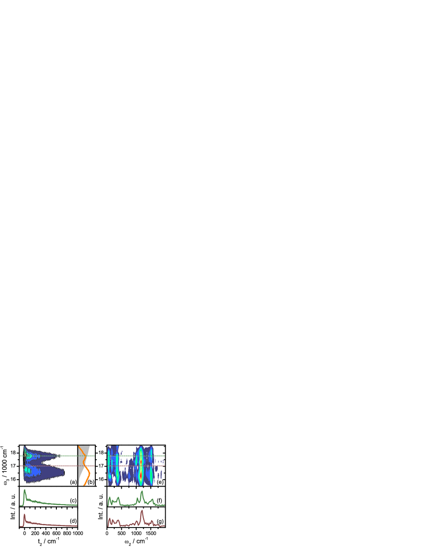
Figure 2: (a) Detection frequency ($\omega{}_{3}$) resolved transient grating signal of LH2 M. pur. (b) Absorption spectrum in gray in comparison to the spectrum of the excitation pulse in orange. Temporal cuts at $S_{2}$-specific detection frequencies specific for $S_{2}$ and $Q_{x}$ in (c) and (d), respectively. (e) Fourier-transform spectra along $t_{2}$, dispersed along $\omega{}_{3}$. (f) and (g) show cuts through (e) for $S_{2}$- and $Q_{x}$-specific detection frequencies, respectively.

III.3 2D electronic spectroscopy

As mentioned in section II, 2D-ES and TG are related in the sense that they are both four wave mixing techniques. The difference lies in the treatment of the first inter-pulse delay $t_{1}$, which is kept at zero in TG, but scanned and Fourier-transformed ($t_{1}\rightarrow\omega_{1}$) in 2D-ES. The emerging ($\omega_{1}$, $\omega_{3}$)-2D plots, recorded at a fixed second inter-pulse delay $t_{2}$, allow for a correlation of excitation ($\omega_{1}$) and emission frequencies ($\omega_{3}$). Fig. 3 compares electronic 2D spectra at $t_{2}$ = 0 fs for the dyad and LH2 M. pur.

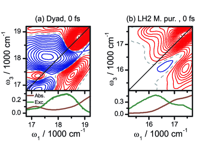
Figure 3: 2D electronic spectra of the dyad (a) and LH2 M. pur., each at $t_{2}$= 0 fs. Positive (negative) signals are drawn a red (blue) full lines at 5% steps. Each figure is normalized to its respective maximum. The dashed grey lines mark the nodal line at zero intensity. The lower panels in each graph show the overlap between absorption (dark red line) and excitation spectrum (green line).

At $t_{2}$ = 0 fs, electronic population is given no time to relax to lower lying states, within experimental time resolution. Both spectra in Fig. 3 show strong positive (red) peaks along the diagonal ($\omega_{1}$=$\omega_{3}$). Comparison to the absorption spectra, given in the lower panels in Fig. 3(a) and (b), show that the strong diagonal peaks stem from the carotenoid’s $S_{0}\rightarrow S_{2}$ transition. The dyad’s spectrum in Fig. 3(a) shows two well resolved peaks corresponding to the $Q_{x}$-transition at approximately 17200 cm^-1 and a carotenoid peak near 19000 cm^-1. The off-diagonal or cross peaks ($\omega_{1}\neq$$\omega_{3}$) with negative amplitude in Fig. 3 stem from ESA-pathways. For carotenoids, ESA from $S_{2}$ in the visible has been observed. Christensson2010a ; Kosumi2005 The ESA of the dyad’s porphyrinic acceptor was described previously as broad and featureless. While the combination of donor and acceptor ESA explains the negative features in the dyad’s 2D-spectrum, we note that at $t_{2}$ = 0 fs, negative signals do not necessarily have to be related to ESA, as they already occur in a two level system at this waiting time. Jonas2003 Positive off-diagonal peaks can stem from vibrational energy levels,Nemeth2010 ; Christensson2011 ; Turner2011a ; Butkus2012 stimulated emission (SE) or coupling between two electronic oscillators.Jonas2003 The latter would be the most interesting scenario, as electronic coupling between donor and acceptor would suggest an excitonic energy level structure and the associated transfer mechanisms.Valkunas2013 Upon visual inspection, the location of the positive cross peaks in the dyad’s 2D signal suggests electronic coupling as a likely explanation. The stronger of the two positive cross peaks, found below the diagonal ($\omega_{1}>\omega_{3}$), peaks at a value of $\omega_{3}$that coincides with the absorption frequency of the $Q_{x}$-band. There is also a corresponding peak above the diagonal ($\omega_{1}<\omega_{3}$), which peaks blue detuned with respect to $Q_{x}$ and with weaker intensity than its counterpart below the diagonal. Such differences in intensity may however be attributed to the ultrafast population transfer from $S_{2}$ to $Q_{x}$, the onset of which takes place within the experimental time resolution of 11 fs. The blue detuned maximum of the upper cross peak can be attributed to finite pulse width or effects of chirp in the excitation pulses. Christensson2010 Inspection of the 2D signal of LH2 M. pur disproves the assumption of electronic coupling. The major difference between the dyad and LH2 M. pur is the position of the $S_{2}$-transition. While the dyad’s carotenoid exhibits maximum absorption above 19000 cm^-1, the carotenoid in LH2 M. pur, okenone, has a carbonyl-containing endgroup as shown in Fig. 1(d), shifting the 0-0 transition of okenone in vivo down to 17570 cm^-1, Andersson1996 while the energetic position of the $Q_{x}$-band remains unchanged between dyad and LH2 M. pur. Hence, the energy difference between $S_{2}$ and $Q_{x}$ should be greatly reduced in LH2 M. pur, and the corresponding cross peaks should be shifted, leading to a large and fairly featureless electronic 2D-signal. In contrast to this expectation, the lower cross peak in LH2 M. pur shows roughly the same energy difference from the diagonal of approximately 1500 cm^-1. This strongly suggest a vibrational origin, given that the prominent C=C stretching mode of carotenoids is found at this energy.

The peak above the diagonal in LH2 M. pur is harder to explain. The ESA-signal in Fig. 3(b) is much weaker than for the dyad case, which is readily explained by a different ESA-transition energy from $S_{2}$ for okenone in vivo. Polli2006 We can thus observe a weak diagonal peak at $\omega_{1}=\omega_{3}\approx$16480 cm^-1, with an excitation frequency $\omega_{1}$ corresponding to the upper cross peak. This energetic position excludes coupling to $Q_{x}$ as a possible explanation, peaking at 17035 cm^-1 in LH2 M. pur. The physical origin of the upper cross peak in Fig. 3(b) becomes more obvious when examining the peak shape evolution along $t_{2}$, as shown in Fig. 4.

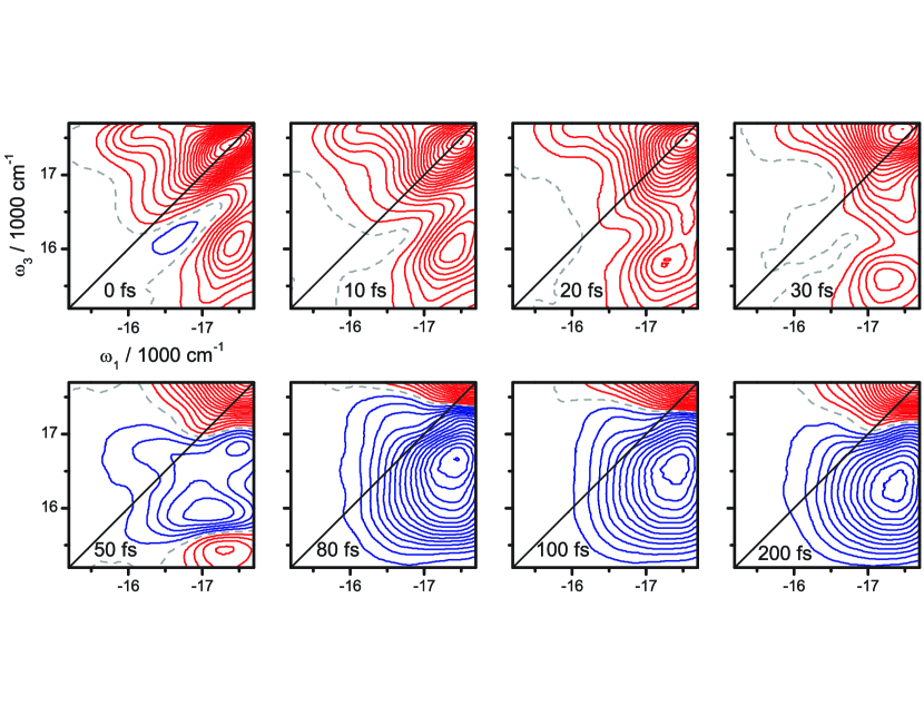
Figure 4: Electronic 2D spectra of LH2 M. pur., measured at indicated values of $t_{2}$. Line coloring follows the same conventions as described in Fig. 3 .

The upper diagonal peak is discernible up to 30 fs, but drops to zero by 80 fs. This behavior is unexpected for an electronic coupling peak, whose amplitude should only be a function of coupling constant J, but not of waiting time $t_{2}$. The rapid decay of the upper cross peak rather suggests that it is an artifact, related to the shape of the excitation pulses. The excitation spectra are clearly non-Gaussian (see lower panel of Fig. 3(b)), making limited pulse width or chirp related effects Christensson2010 the most likely explanation for the upper diagonal cross peak for LH2 M. pur.

Another interesting feature is observed at ($\omega_{1}$ = -17500 cm^-1, $\omega_{3}$ = 16480 cm^-1), i.e. an energetic position indicative of $S_{2}\rightarrow Q_{x}$ energy transfer pathways. The peak builds up rapidly within the first 30 fs, which corresponds well with the 55 fs transfer time reported for this process.Polli2006 After 50 fs, negative ESA-signals dominate the spectra. This is explained by the intramolecular $S_{2}\rightarrow S_{1}$ energy transfer, occurring at a 95 fs build up rate as reported previously.Polli2006 We support this assignment by calculating the electronic 2D-spectra only for okenone, the carotenoid of LH2 M. pur. Details of the calculations can be found in section IIC.

IV Discussion

IV.1 Carotenoid-Chlorophyll Interaction

Spectroscopic experiments reveal the transfer from Car $S_{2}$ and $S_{1}$ states to Chls and BChls as fast and relatively efficient despite the rather short $S_{2}$ state life time of the monomeric carotenoid (at least in comparison with Chls and BChls). Both $Q_{x}$ and $S_{2}$ states are optically allowed, and they can therefore interact by the resonance coupling mechanism. Because of the proximity of the two molecules in the LH2 structure, one cannot exclude an electron exchange (Dexter) mechanism. However, quantum chemical calculations suggest Coulomb interaction to be dominant here Nagae1993 . In this case, theoretical description the carotenoid-BChl interaction and modeling of the corresponding excitation energy dynamics remain within the well understood framework of excitonic description of photosynthetic antennae VanAmerongen2000 ; Valkunas2013 .

In the standard framework, we assume the electronic coupling element between the two electronic states to be independent of the vibrational DOF of the molecular system. Electronic excitation is transferred between the two molecules due to an interplay of the resonance coupling and the fast fluctuations of the molecules’ respective energy gaps. The energy gap fluctuations are caused by their interaction with the nuclear degrees of freedom (DOF) which involve both the intra- as well as intermolecular vibrations. These are considered a thermodynamic heat bath characterized by certain temperature and spectral density. Two regimes of the relative coupling strengths are usually distinguished. The delocalized regime in which the system-bath interaction is weak in comparison with the resonance interaction between the molecules, and the localized regime in which the system-bath coupling is considered strong. The terms localized and delocalized refer to the effective electronic eigenstates of the interacting system. For the delocalized regime the coupling between the two molecules is strong enough to sustain correlation between the electronic excitations on different molecules so that delocalized excitons are formed. In the localized regime (also referred to as Förster regime here), the system-bath interactions induce energy gap fluctuations which prevent any such correlation, and the excitations appear to be localized on the molecules. In fact, even in relatively weakly excitonically coupled systems one can often detect signs of delocalization (see e.g. Ref. Cheng2006 ), because the actual apparent eigenstates are always somewhere in between the two theoretical limits. For photosynthetic aggregates formed by BChl and Chl molecules, where the protein bath can be to some extent assumed as unstructured, modern simulation methods such as the Hierarchical Equations of Motion (HEOM) enable us to determine the excited state dynamics beyond the two limits mentioned above.Ishizaki2009 However, even in the case of aggregates composed of BChl or Chl molecules only, some clearly visible spectroscopic features can result from the involvement of pronounced vibrational modes. Christensson2012 ; Tiwari2013 ; Chin2013 ; Chenu2013

In the discussion that follows, we want to argue that the involvement of the vibrational DOF of the carotenoid molecules is crucial for the energy transfer dynamics between the $S_{2}$ and the $Q_{x}$ states. We will compare two theoretical approaches to the calculation of the energy transfer rates, both motivated by the observed features of the spectra and known spectroscopic behavior of the system. We will argue that both support the crucial role of the fast vibrational modes, in particular the carotenoid ground state vibration levels.

The Hamiltonian of the relevant part of the system (state $Q_{X}$ of the BChl and the $S_{2}$ state of the carotenoid) can be written in the following way

$$H=H_{Q_{x}}^{(B)}+H_{S_{2}}^{(B)}+\left(\epsilon_{Q_{x}}+\Delta V_{Q_{x}}(q^{(Q_{x})})\right)|Q_{x}\rangle\langle Q_{x}|$$

$$+\left(\epsilon_{S_{2}}+\Delta V_{S_{2}}(q^{(S_{2})})\right)|S_{2}\rangle\langle S_{2}|$$

$$+J\left(|S_{2}\rangle\langle Q_{x}|+|Q_{x}\rangle\langle S_{2}|\right).$$ (6)

Here, $\epsilon_{Q_{x}}$ and $\epsilon_{S_{2}}$ are the optical electronic transition energies of the BChl $Q_{x}$ state and the carotenoid $S_{2}$ state, respectively (including the reorganization energy of the bath), $H_{Q_{x}}^{(B)}$ and $H_{S_{2}}^{(B)}$ are the Hamiltonian operators of the nuclear DOF on the BChl and carotenoid, respectively. These two sets on nuclear DOF described by macroscopic sets of coordinates $q^{(Q_{x})}=\{q_{1}^{BChl},\dots,q_{n}^{BChl}\text{\}}$ and $q^{(S_{2})}=\{q_{1}^{Car},\dots,q_{n}^{Car}\}$, where $n$ is a macroscopically large number, form the bath interacting through operators $\Delta V_{Q_{x}}(q^{(Q_{x})})$ and $\Delta V_{S_{2}}(q^{(S_{2})})$ with the electronic transitions on the BChl and carotenoid, respectively. The electronic coupling element $J$ describes the resonance interaction between the collective excited state $|Q_{x}\rangle=|e_{Q_{x}}\rangle|g_{Car}\rangle$ in which the BChl is excited to the state $Q_{x}$ and the carotenoid is in its electronic ground state and the collective excited state $|S_{2}\rangle=|g_{BChl}\rangle|e_{S_{2}}\rangle$ in which the BChl is in its electronic ground state and the carotenoid is excited to its excited state $S_{2}$. To complete the Hamiltonian we should also to include the state $|f\rangle=|e_{Q_{x}}\rangle|e_{S_{2}}\rangle$ in which both Car and BChl are excited. However it will be shown later that the features related to this state are negligible as the resonance coupling will be shown to be weak. In the experimental 2D spectra, shown in Fig. 4, one can easily identify the fast rising ESA component, which is usually assigned to the strong absorption from the $S_{1}$ states of the carotenoid. Contribution of this state is taken into account by including a separate partial Hamiltonian and $S_{2}\rightarrow S_{1}$ relaxation rate into the response functions in Appendix A All other states with no spectroscopic contributions are taken into account in the simulations by introducing decay rates for the bright states. For the subsequent discussion it will be useful to introduce a bare electronic (single exciton) Hamiltonian which reads as

$$H_{{\rm el}}=\epsilon_{Q_{x}}|Q_{x}\rangle\langle Q_{x}|+\epsilon_{S_{2}}|S_{2}\rangle\langle S_{2}|$$

$$+J\left(|S_{2}\rangle\langle Q_{x}|+|Q_{x}\rangle\langle S_{2}|\right).$$ (7)

This Hamiltonian represents the basic three level (ground state energy was chosen to be zero) structure of the problem.

IV.2 Energy Transfer Rates

As discussed above, the interplay of energy gap fluctuations and the resonance coupling energy determines which theoretical limit applies. The usual discussion of the relative strengths of the two interactions is made based on the relative values of the reorganization energy $\lambda$ which describes the magnitude of the energy gap fluctuations and the value of the resonance coupling $J$ Ishizaki2009a . Our system is characterized by reorganization energies $\lambda_{Q_{x}}$ of the BChl and $\lambda_{S_{2}}$ of the Car which should be compared to the resonance coupling energy $J$. For the validity of the weak resonance coupling limit it is usually required that $\lambda>|J|$. In our case, assuming $J\approx 100$ cm^-1 (see Ref. Tretiak2000 ; Krueger1998 ) confirms the validity of this regime because the total $\lambda_{S_{2}}$ is in the order of thousands of cm^-1 as it involves two fast vibrational modes with Huang-Rhys factors close to $1$ and vibrational frequencies above $1000$ cm^-1 as shown in Fig. 2. The $Q_{y}$ state of BChl in the protein environment of the LH2 complex exhibits $\lambda_{Q_{y}}\approx 100$ cm^-1 (see e.g. Ref. Zigmantas2006 ) and we can assume a similar value $\lambda_{Q_{x}}\approx 100$ cm^-1 as for the $Q_{x}$ state. Here, the reorganization energy of the chromophore is only comparable, not larger, than the resonance coupling element. We note that conventionally the role of temperature is completely neglected in this discussion. The magnitude of the energy gap correlation function, which provides a true measure of the energy gap fluctuations, depends on temperature and the dependency is linear in the high temperature limit (in the case of Brownian oscillator model, see Ref. Mukamel1995 ). It would therefore be more suitable to compare the value of $\lambda k_{B}T$ and $|J|^{2}$. At room temperature, $k_{B}T=207$ cm^-1 and $\lambda_{Q_{x}}k_{B}T>|J|^{2}$. Yet another problem arises when considering the role of the relative energy gap $\Delta\varepsilon=\epsilon_{S_{2}}-\epsilon_{Q_{x}}$ of the $Q_{x}$ and $S_{2}$ states. In an ideal dimer, the delocalization is determined by the so-called mixing angle $\theta=\frac{1}{2}\arctan\frac{2|J|}{|\Delta\epsilon|}.$May2000 The delocalization decreases with the increasing $\Delta\varepsilon$. The interplay of the relative energy gap, temperature, reorganization energy and resonance energy is a subject of numerous theoretical studies in the context of photosynthesis. However, no simple formula taking into account the influences of all these parameters on the degree of delocalization exists.

After the discussion of the parameters of the carotenoid-BChl dimer, we have many reasons to believe that the interaction of the $S_{2}$ and $Q_{x}$ states can be treated in the weak coupling limit. The issues is however more complicated because of the nature of the system-bath interaction in the carotenoid. Most of its reorganization energy can be assigned to the fast intramolecular vibrational modes. The spacing between the vibrational levels and the relative electronic energy gap $\Delta\varepsilon$ are such that the $Q_{x}$ state can be viewed as effectively interacting with the nearest vibrational levels and not with the carotenoid electronic state as a whole. This is a situation similar to the one studied in Refs. Christensson2012 ; Chin2013 ; Chenu2013 where special resonances between vibrational and electronic energy gaps lead to pronounced effects despite the small Huang-Rhys factors of the BChls. Clearly, treating the carotenoid vibrations as a thermodynamic bath is a questionable approximation.

In the following subsections we will briefly discuss the carotenoid-BChl energy transfer rates based on the weak coupling Förster theory, and compare it with an explicit treatment of the carotenoid vibrations in the Hamiltonian, along with Refs. Christensson2012 ; Chenu2013 . The energy level structure characteristic for the two situations is presented in Fig. 5.

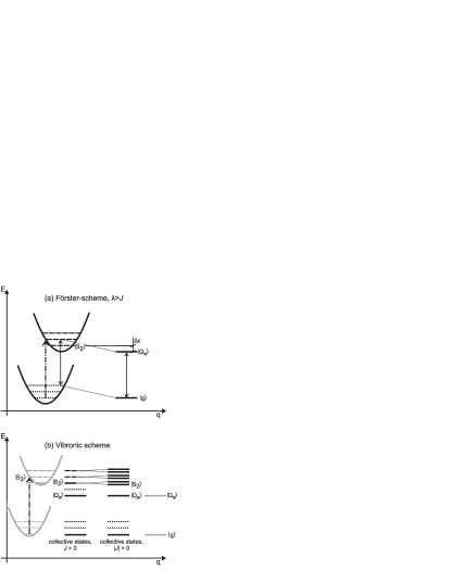
Figure 5: Interaction schemes of the electronic and vibrational levels in (a) localized (Förster) and (b) delocalized (vibronic) regime. In the case (a) the transition energy from the non-equilibrated state of the carotenoid excited state vibrations has to be resonant with the $Q_{x}$ transition energy. The relative energy gap $\Delta\varepsilon$ between the $S_{2}$ and $Q_{x}$ transitions requires involvement of more than one vibrational quanta of the carotenoid. The vibronic case (b) also involves excitonic mixing of the vibrational levels of the carotenoid with the $Q_{x}$ transition. The collective single excited states of the carotenoid-purpurin or carotenoid-BChl dimer involve states in which the $Q_{x}$ transition is excited and simultaneously the electronic ground state vibrations of the carotenoid are excited. The states can excitonically mix with the carotenoid electronically excited state with a different number of vibrational quanta.

IV.2.1 Weak Resonance Coupling Limit

In the weak resonance coupling limit, the parameter $J$ of the Hamiltonian, Eq. (6), is assumed small and perturbation theory to the second order can be performed. For two transitions (donor and acceptor), the transition rate is given by the Fermi golden rule as$K_{A\leftarrow D}=\frac{2\pi}{\hbar}|J|^{2}\delta(\epsilon_{D}-\epsilon_{A}).$ It is possible to view the donor molecule as a set of many available de-excitation transition (the molecule is excited electronically and vibrationally) while the acceptor molecule can be viewed as a set of transitions ready to be excited. In a realistic case it is therefore necessary to integrate the Fermi formula over all acceptor and donor transitions

$$K_{A\leftarrow D}=\frac{2\pi}{\hbar}|J|^{2}$$

$$\times\int\limits_{-\infty}^{\infty}{\rm d}\epsilon_{D}\int\limits_{-\infty}^{\infty}{\rm d}\epsilon_{A}f_{{\rm abs}}(\epsilon_{A})f_{{\rm fl}}(\epsilon_{D})\delta(\epsilon_{D}-\epsilon_{A}),$$ (8)

where $f_{{\rm abs}}$ and $f_{{\rm fl}}$ correspond to the normalized distribution of the transition energies available for excitation on the acceptor and the normalized distribution of the transition energies available for the deexcitation on the donor. The Förster rate can be derived directly from Eq. (8) by noticing that the acceptor absorption spectrum is related to the distribution of transition frequencies $\tilde{f}_{{\rm abs}}(\omega)=f_{{\rm abs}}(\hbar\omega)$ as $\alpha(\omega)\sim\omega\tilde{f}_{{\rm abs}}(\omega)$ and similarly for the donor fluorescence spectrum $\sigma(\omega)\sim\omega^{3}\tilde{f}_{{\rm fl}}(\omega)$ (see e.g. VanAmerongen2000 ; May2000 ) or directly by perturbation theory with respect to $J$ and a cumulant expansion for the bath DOF as in Ref. Valkunas2013 . In both cases there is a direct relation between the rate and the overlap of absorption spectrum of the acceptor with the emission spectrum of the donor

$$K_{A\leftarrow D}=2\pi\frac{|J|^{2}}{\hbar^{2}}\frac{\int d\omega\alpha_{A}(\omega)\sigma_{D}(\omega)\omega^{-4}}{\int d\omega\alpha_{A}(\omega)\omega^{-1}\int d\omega\sigma_{D}(\omega)\omega^{-3}}.$$ (9)

It is important to note that the Förster theory does not in general depend on the dipole-dipole coupling approximation although the specific dependence of the rate in this approximation is often used. From the point of view of the present manuscript, the coupling energy $J$ can be calculated by any type of advanced methods of quantum chemistry which takes into account all the details of the electronic structure of the excited states of the interacting molecules Scholes2003 . From the theoretical point of view, the Förster rate can be derived from Hamiltonian, Eq. (6), under various assumptions. Usually one assumes relaxed state of the environment and the intramolecular vibrational modes. However, Förster theory is very versatile and allows many generalizations Scholes2003 ; Beljonne2009 , most importantly it is still valid for the case that the excited state of the donor is unrelaxed Mukamel1995 . Eq. (8) is then still valid, but it does not result in Eq. (9). Förster theory therefore also allows for a direct experimental estimation of the resonance coupling if the fluorescence spectrum of the donor and the absorption spectrum of the acceptor are known, even in case that the fluorescence does not start from a relaxed state. For the present dyad, the coupling $J$ was determined to be $J=240$ cm^-1, within the framework of Eq. (9). Macpherson2002

Fig. 5(a) describes a typical situation for the short time dynamics of the $S_{2}-Q_{x}$ energy transfer. The higher vibrationally excited levels of the $S_{2}$ are populated, and in order to achieve resonance with the $Q_{x}$ transition, even higher vibrational levels on the carotenoid ground state are excited after deexcitation of the donor ($S_{2}$). The energy transfer is enabled by the fact that the energy corresponding to the $\Delta\varepsilon$ is accepted by the ground state vibrational levels of the carotenoid molecule as depicted in Fig. 5(a). The same statement can be rephrased in terms of the spectral overlap. Because the rate depends on the overlap of the donor emission and the acceptor absorption spectra, the effective broadening of the carotenoid spectrum due to the fast vibrational modes increases significantly the energy transfer rate. Förster theory thus assigns the electronic ground state vibrational levels of the carotenoid a crucial importance in the energy transfer process.

IV.2.2 Vibronic Coupling

The main conclusion of the preceding section is that the vibrational modes of the carotenoid are the main driving element of the energy transfer from $S_{2}$ to $Q_{x}$. Förster theory shows that these modes provide resonance for the energy transfer and that this resonance involves multiple vibrational quanta. As one can learn from Fig. 1(a), absorption lineshape undergoes a slight change in the carotenoid region suggesting weak delocalization between $Q_{x}$ and $S_{2}$ states, at least for dyad. It is therefore natural to include the important vibrational modes explicitly into the Hamiltonian, and to treat only the remaining overdamped modes as a bath. This leads directly to the model of vibronic excitons (see Refs. Womick2011 ; Christensson2012 ; Tiwari2013 ; Chin2013 ). Such a model automatically treats the selected vibrational modes non-perturbatively.

We split the nuclear part of the carotenoid Hamiltonian in Eq. (6) into some selected modes denoted by coordinates $\tilde{q}_{n}$ and referred to later in the text as primary modes. The rest of the modes which we denote by $q^{\prime(S_{2})}$ (see Sec. IV.1 for the notation) will be referred to as secondary modes or secondary bath. We have

$$H_{S_{2}}^{(B)}=H_{S_{2}}^{(b)}+H_{{\rm vib}}+H_{{\rm vib-b}}.$$ (10)

where $H_{S_{2}}^{(b)}$ is the Hamiltonian of the secondary bath and the Hamiltonian of the primary modes and their interaction with the secondary bath read as

$$H_{{\rm vib}}=\sum_{n}\frac{\hbar\tilde{\omega}_{n}}{2}\left(\tilde{p}_{n}^{2}+\tilde{q}_{n}^{2}\right),$$ (11)

and

$$H_{{\rm vib-b}}=-\sum_{n}\tilde{q}_{n}\sum_{k}\xi_{k}^{n}q_{k}.$$ (12)

Here, $\tilde{\omega}_{n}$ are the frequencies of the primary modes to be treated explicitly, and $q_{k}$ are the coordinates from the set $q^{\prime(S_{2})}$ coupled to the primary modes by some coupling constants $\xi_{k}^{n}$. In the excited state of the carotenoid, the bath Hamiltonian is now split in the following way

$$H_{S_{2}}^{(B)}+\Delta V_{S_{2}}(q^{(S_{2})})=H_{S_{2}}^{(b)}+\Delta V_{S_{2}}(q^{\prime(S_{2})})$$

$$+\sum_{n}\frac{\hbar\omega_{n}}{2}\left(\tilde{p}_{n}^{2}+(\tilde{q}_{n}-d_{n})^{2}\right)-\sum_{n}(\tilde{q}_{n}-d_{n})\sum_{k}\xi_{k}^{n}q_{k}.$$ (13)

Here, we assume that the same secondary bath which drives the ground state vibrations into the equilibrium, drives also the excited state vibrations to their corresponding equilibrium. Correspondingly, the energy gap operator reads as

$$\Delta V_{S_{2}}(q^{(S_{2})})=\Delta V_{S_{2}}(q^{\prime(S_{2})})$$

$$-\sum_{n}\hbar\tilde{\omega}_{n}d_{n}\tilde{q}_{n}+\sum_{n}d_{n}\sum_{k}\xi_{k}^{(n)}q_{k}.$$ (14)

We assumed that the spectral densities describing the interaction of the selected modes with the rest of the bath are the same. The energy gap operator, Eq. (14), is composed of three parts, $\Delta V_{S_{2}}(q^{\prime(S_{2})})$ representing the overdamped bath, the part representing the direct influence of the selected modes on the energy gap fluctuations

$$H_{{\rm el-vib}}=\sum_{n}\hbar\tilde{\omega}_{n}d_{n}\tilde{q}_{n},$$ (15)

and the part describing the influence of the overdamped bath on the electronic energy gap functions via the coupling with the selected modes. The strength of the latter part of the interaction Hamiltonian is given by the shift $d_{n}$ of the excited state vibrational potential with respect to the ground state potential. The essence of the vibronic model is to include $H_{{\rm el-vib}}$ to the Hamiltonian which we treat explicitly and only an effective energy gap operator

$$\Delta V_{S_{2}}^{({\rm eff)}}(q^{\prime(S_{2})})=\Delta V_{S_{2}}(q^{\prime(S_{2})})+\sum_{n}d_{n}\sum_{k}\xi_{k}^{(n)}q_{k}$$ (16)

is treated by perturbation theory. It leads to the bath correlation function

$$C(t)=\langle\Delta V_{S_{2}}(q^{\prime(S_{2})};t)\Delta V_{S_{2}}(q^{\prime(S_{2})};0)\rangle+C_{{\rm b}}^{({\rm el})}(t),$$ (17)

where the last term on the right hand side corresponds to the direct contribution of the secondary bath to the dephasing. The damping of the $n$th primary modes is governed by the bath correlation function originating from the term, Eq. (12),

$$C_{{\rm b}}^{(n)}(t)=\sum_{k}|\xi_{k}^{n}|^{2}\langle q_{k}(t)q_{k}\rangle,$$ (18)

while the direct contribution of the secondary bath to the dephasing is expressed by the same correlation function scaled by the dimensionless shift of the effective vibrational mode

$$C_{{\rm b}}^{({\rm el})}(t)=\sum_{n}|d_{n}|^{2}C_{{\rm b}}^{(n)}(t).$$ (19)

The calculation of the energy transfer dynamics in the vibronic model thus starts with a diagonalization of the Hamiltonian

$$H_{S}=H_{{\rm vib}}+H_{{\rm el-vib}}|S_{2}\rangle\langle S_{2}|+H_{{\rm el}}.$$ (20)

The diagonalization results in eigenstates which combine the electronic and vibrational states into the mixed vibronic states. In a second step the rates of population transfer and coherence dephasing are calculated for the set of eigenstates by second order perturbation theory and cumulant expansion Perlik2014 using correlation function, Eq. (18), for the damping of the selected mode and the correlation function $C_{{\rm b}}^{({\rm el})}(t)$ only to simulate electronic dephasing. This means that we assume the correlation function $C(t)$, Eq. (17), to be composed of the contribution of the secondary bath only. This choice decreases the number of degrees of freedom in fitting and effectively ties strength of the coupling between the primary mode and the secondary bath to the strengths of the interaction between the electronic transition and the primary mode. Because only effective spectral density is important for the calculation of the transition rates, we believe that the advantage in limiting the number of parameters outweighs the restriction put on our model. In principle one could estimate the overall rate of energy transfer directly by weighting the calculated rates between individual levels. We have however chosen the more practical approach of calculating the transfer time as described in Section II.3.2.

Because of the rather large vibrational frequency and moderate coupling, the $Q_{x}$ transition can be viewed as interacting only with the energetically nearest transition. This situation is depicted in Fig. 5(b). For the sake of clarity of the graphical presentation, we depict a situation of perfect resonance between the relative energy gap $\Delta\varepsilon$ and the vibrational frequency and show energy level splitting of the energetically nearest levels. Fig. 5b depicts the relevant carotenoid and BChl energy levels as two separate entities (in gray) and in terms of collective states of the carotenoid-BChl dimer in the case of $J=0$. Conceptually, the ground state vibrational levels of the carotenoid contribute to an excited collective state if the $Q_{x}$ state is excited. This is a consequence of the fact in a singly excited aggregate state all molecules except one are in their ground state (carotenoid in this case). The ground state vibrational levels of the carotenoid thus interact resonantly with the vibrational levels of the carotenoid in the electronically excited state $S_{2}$. This interaction corresponds to the energy transfer from $S_{2}$ to $Q_{x}$ with a simultaneous deposition of the excess energy to the ground state vibrations of the carotenoid. The complete picture of the energy levels of the system is much more complicated because the excitonic mixing involves all available states. The details of this mixing, which are included in the basis transformation from the localized states to the energetic eigenstates, lead to discernible changes in the lineshape of the carotenoid molecule. As will be demonstrated in the following sections, the vibronic model provides an explanation for the observed spectral changes as shown in Fig. 1(a). Also, the detailed treatment of the interaction between carotenoid vibrational levels and the $Q_{x}$ state leads to the experimentally observed energy transfer rates with a significantly weaker resonance coupling than predicted by Eq. (9).

IV.3 Simulation of Absorption Spectra and Transfer Rates in Vibronic Model

The vibronic model discussed in the previous section was implemented as described in Section II.3.2. The absorption spectra of monomeric carotenoid was fitted with a model Hamiltonian involving one effective high frequency mode to obtain starting values of the effective mode parameters for the subsequent fitting of the absorption spectra of the dyad and the LH2 complex. We found the frequency of the vibrational mode in the dyad to be $\omega_{{\rm eff}}=1390$ cm^-1 and its Huang-Rhys factor was determined to be $s_{{\rm eff}}=1.3$. All monomeric parameters are discussed in Section II.3.2.

In Fig. 6 we summarize our fitting efforts for the dyad. We chose the dyad because the same solvent can be used for the dyad and its components avoiding solvent related bathochromic shifts. The absorption spectra of LH2 M. pur. and LH2 Rps. ac. were equally well reproduced with the employed vibronic model. Fig. 6(a) presents the result of summation of the dyad’s monomer spectra. This is the spectrum corresponding to the weak resonance coupling case (Förster regime) and it is presented to highlight the changes between monomeric and dyad spectra. In Fig. 6b, we present a result of the fitting in which the Huang-Rhys factor of the carotenoid, the $Q_{x}$ transition frequency, the relative energy gap $\Delta\varepsilon$ between $S_{2}$ and $Q_{x}$ and the resonance coupling $J$ were allowed to change. The fitting achieves good agreement with the experimental dyad spectrum, most importantly in the carotenoid related part. There the relative hight of the absorption maxima of different vibrational peaks changes between the monomer and the dyad. The estimated coupling is $J=-119$ cm^-1 while $s_{{\rm eff}}=1.29$, $\Delta\varepsilon=2400$ cm^-1 and $\epsilon_{Q_{x}}=17150$ cm^-1. The minor change with respect to the parameters of the monomers, such as the change of the transition energy to the excited state, have to be assigned to the chemical change upon formation of the dyad.Macpherson2002

The same fitting procedure with the fixed resonance coupling $J$ estimated from measured fluorescence spectrum by Förster theory, $J=240$ cm^-1 Macpherson2002 , results in a less satisfactory agreement as can be seen in Fig. 6(c). In order to demonstrate that lineshape changes in all cases are not only due to the change of the monomeric Huang-Rhys factor of the carotenoid molecule, we show the spectrum of the dyad with the parameters resulting from the same parameters but with $J=0$ cm^-1 in Fig. 6(d). Interestingly, the best fit is achieved with a change of the Huang-Rhys factor of less than $1$ % and the change in the line shape can be therefore mostly assigned to the resonance coupling.

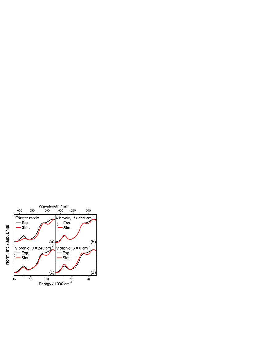
Figure 6: Absorption spectra of the dyad. Panel (a) shows the sum of the monomeric spectra, which corresponds to the weak coupling case (no changes to the lineshape except of lifetime broadening); (b) presents the best fit of the dyad spectrum with the $Q_{x}$ transition energy, relative energy gap $\Delta\varepsilon$, carotenoid HR factors and the resonance coupling free to be adjusted. Panel (c) shows the best fit with the resonance coupling fixed at $J=240$ cm^-1 and panel (d) presents the sum of the monomers with the parameters corresponding to the best fit from panel (b), but with $J=0$ cm^-1.

The simulation of the absorption spectrum has resulted in a value of $J$ which is by $50$ % smaller than the one estimated from the experiment, suggesting that higher value is not compatible with the spectral changes with respect to the monomers seen in the dyad. The obvious question is whether this lower value for the resonance coupling is compatible with the measured ultrafast rates. To this end we perform calculations of the $S_{2}$ to $Q_{x}$ transfer dynamics to estimate the transfer time introduced in Section II.3.2 for various values of $J$ and $\Delta\varepsilon$ and keeping other parameters of the model fixed to those from the best fit from Fig. 6(b). The plot of transfer time as a function of $J$ and $\Delta\varepsilon$ is presented in Fig. 7. The calculations yield a transfer time of $\tau_{S_{2}\rightarrow Q_{x}}=55$ fs for the values of the best fit which is in good agreement with the experimental value of $40$ fs.Macpherson2002 Moreover the 2D plot in Fig. 7 and the corresponding cut at the value of $J=-119$ cm^-1reveals a periodic modulation of the transfer time with the period corresponding to the effective spacing between vibrational levels. The transfer time decreases monotonically with increasing value of $J$, as shown in the lower panes of Fig. 7 representing cuts along the experimental vales of $\Delta\varepsilon$. The periodic modulation of the transfer time is in agreement with the resonant involvement of the carotenoid vibrational modes in the energy transfer. As in the Förster case this implies the involvement of the carotenoid vibrational levels from the electronic ground state. Conservation of energy during the energy transfer requires the excess energy to be deposited to the vibrational energy of the carotenoid.

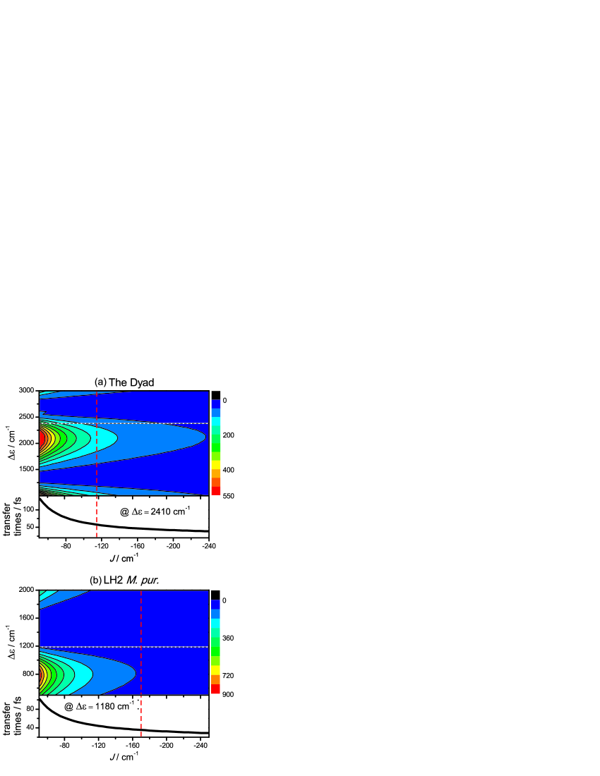
Figure 7: Transfer time as a function of $J$ and $\Delta\varepsilon$ for the dyad (a) and for LH2 M. pur. (b). At the experimental value of $\Delta\varepsilon$ and the values of resonance coupling determined by fitting absorption spectrum, transfer time for the dyad and LH2 M. pur. are 55 fs and 40 fs, respectively, in agreement with the values reported in pump probe measurements.

IV.4 Simulation of the 2D Spectra

In order to assign the observed features of the experiment 2D-spectrum we performed simulations of the carotenoid 2D spectra. This is a first step towards a complete simulation of the interacting Car-BChl system, which allows us to assign Car only features and possibly identify 2D spectral components originating in $Q_{x}$ state. Such a full calculation will be a subject of our future work.

Calculating the 2D spectrum in a spectral region covering the edge of the studied molecule is an extremely difficult task given the fact that a good fit on the outer region of (even the absorption) spectrum depends on many rarely studied details of the chromophore interaction with its environment. For instance, assumptions about the Gaussian disorder of the electronic transitions energies and typical estimates for bath spectral densities are well suited for explaning the features around the maximum of absorption and do not cover well the situation at the edges of the spectra. On the other hand, introducing more fitting freedom by assuming arbitrarily some other types of spectral densities and disorder distributions seems not to yield more theoretical insight, as the new parameters cannot be fixed by a limited set of experiments. Below we therefore describe a calculation of the Car 2D-spectra in which the Car molecule should well represent the Car component of the LH2. Correspondingly a limited fitting to the experiment 2D-spectra from Fig. 4 is done, keeping in mind that the two systems which are compared in such a fitting are different. Large part of the Car parameters are therefore motivated by the values from literature.

IV.4.1 Carotenoid only Spectra

From the linear absorption spectrum of the LH2 complex the electronic excitation energy $\omega_{S_{2}S_{0}}=19770\,\mathrm{cm^{-1}}$ was obtained (see Fig. 1). Because of the line shape function approach, which relies on second-order cumulant expansion with the electronic ground state as the reference state, this value corresponds to the vertical transition energy, i.e. the sum of the electronic excitation energy and the reorganization energies of the spectral density components. The transfer rates were chosen under the assumptions $1/k_{S_{2}\to S_{1}}=95\,\mathrm{fs}$ and $1/k_{S_{2}\to Q_{x}}=55\,\mathrm{fs}$ in agreement with PoCeLa06_BPJ_2086 . Because of the slow transfer from $S_{1}$ to other electronic states, the lifetime broadening constant $\Gamma_{S_{1}}$ was taken as zero. Even though some spectral density parameters for okenone are available from the literature PoCeLa06_BPJ_2086 , the respective parameters for $\beta$-Carotene have been reported in more detail. They can at least provide some orientation for the choice of the parameters to model the okenone component of the investigated LH2 complex. According to ChZiMa13_JCP_11209 the frequencies of the included vibrational modes are $\omega_{UO,1}=1150\,\mathrm{cm^{-1}}$ and $\omega_{UO,2}=1520\,\mathrm{cm^{-1}}$. The Huang-Rhys factors of the vibrational modes in $S_{2}$ were assumed as $\chi_{UO,S_{2}S_{2},1}=0.25\,\mathrm{}$ and $\chi_{UO,S_{2}S_{2},2}=0.5\,\mathrm{}$. While these values are somewhat smaller than the ones for $\beta$-Carotene given in Ref. ChZiMa13_JCP_11209 , their ratio is similar. According to the tendency reported in the literature, the Huang-Rhys factors in $S_{1}$ were assumed to be larger than those in $S_{2}$ by a scaling factor chosen as 1.5 . To describe the damping of the vibrational modes in $S_{1}$ with a time constant of $50\,\mathrm{fs}$, ten Matsubara terms were taken into account in the calculation of the lineshape function. For one of the Brownian oscillator spectral density components a fast decay with damping constant $1/\Lambda_{BO1,S_{2}S_{2}}=30\,\mathrm{fs}$ and a reorganization energy $\lambda_{BO,S_{2}S_{2},1}=300\,\mathrm{cm^{-1}}$ in agreement with Ref. ChMiNe09_JPCB_16409 was assumed. To reproduce the inhomogeneous broadening effects in the absorption spectrum of the LH2 complex, the second Brownian oscillator spectral density component with very slow decay constant of $20\,\mathrm{ps}$ ChMiNe09_JPCB_16409 was included in the model. For a reorganization energy of $\lambda_{BO,S_{2}S_{2},2}=3000\,\mathrm{cm^{-1}}$ comparable inhomogeneous broadening effects as in a measured linear absorption spectrum could be obtained and features in the measured 2D-spectra could be qualitatively reproduced. In Ref. SuYaCo07_PRB_155110 it has been reported that coherence gets lost during this population transfer process, so that the fluctuations in $S_{2}$ and $S_{1}$ can be considered as uncorrelated. Accordingly, $g_{S_{2}S_{1}}$ and $g_{S_{2}S_{n}}$ were taken as zero. The Huang-Rhys factors for excitation from $S_{1}$ to $S_{n}$ are known to be much smaller than the ones of the excitation from $S_{0}$ to $S_{2}$. In Ref.PoCeLa06_BPJ_2086 a value of $0.1\,\mathrm{}$ is given, which was assumed for both modes in our calculation.

According to our interpretation, this value of the Huang-Rhys factor is given with respect to $S_{0}$, as the vibrational energy for the transition between $S_{1}$ and $S_{n}$ reported in Ref. PoCeLa06_BPJ_2086 cannot be explained by such a small Huang-Rhys factor. However, the much larger Huang-Rhys factors of $S_{1}$ with respect to $S_{0}$ allows for a larger vibrational energy than expected from the value of $0.1$ for the Huang-Rhys factor.

Regarding the Brownian oscillator modes, it has been reported in ChMiNe09_JPCB_16409 that for double excitation from $S_{1}$ the reorganization energy corresponds to a fraction of only $0.5\,\mathrm{}$ of the corresponding reorganization energy in $S_{1}$ from the electronic ground state, which was taken as the same as for $S_{2}$ in our description.

The vertical transition energy between $S_{1}$ and $S_{n}$ was chosen as $\omega_{S_{1}S_{n}}=15400\,\mathrm{cm^{-1}}$ in agreement with Ref. PoCeLa06_BPJ_2086 . In the prefactors of the ESA response functions $\left|\frac{\mu_{S_{1}S_{n}}}{\mu_{S_{0}S_{2}}}\right|^{2}=1.5\,\mathrm{}$ entered, following the values given in ChPoYaPu09_PRB_245118 for other carotenoid derivatives. The finite pulse widths were taken into account in terms of Gaussian profiles determined from a fit of the measured local oscillator spectrum . In this way the central frequency $\omega_{0}=16275\,\mathrm{cm^{-1}}$ and a FWHM of $1612\,\mathrm{cm^{-1}}$ were obtained. As the fitted curve corresponds to the squared pulse profile, multiplication of the FWHM with a factor of $\sqrt{2}$ was required to obtain the FWHM of the single pulses with a value of $2280\,\mathrm{cm^{-1}}$.

In the real part of the sum of all calculated response function contributions after convolution with the pulses an intensive, positive-valued diagonal peak in the region of ($\omega_{1}=-17500\,\mathrm{cm^{-1}}$,$\omega_{3}=17500\,\mathrm{cm^{-1}}$) appears at all population times up to $100$ fs, starting from $t_{2}=0\,\mathrm{fs}$. This peak mainly stems from the rephasing GSB contribution. Furthermore, below the diagonal at ($\omega_{1}=-17500\,\mathrm{cm^{-1}}$,$\omega_{3}=16000\,\mathrm{cm^{-1}}$)a crosspeak from the rephasing GSB contribution is found, which stems from vibrational effects. This initially oval peak becomes butterfly-shaped with a nodal line separating positive an negative region at $t_{2}=10\,\mathrm{fs}$, whereas at $t_{2}=20\,\mathrm{fs}$ it becomes completely positive again. At $t_{2}=30\,\mathrm{fs}$ a modified shape of the vibrational crosspeak below the diagonal from the rephasing GSB contribution in combination with a rise of of the rephasing SE contribution and the negative-valued rephasing ESA contribution leads to a localization of the crosspeak close to ($\omega_{1}=-18000\,\mathrm{cm^{-1}}$,$\omega_{3}=15500\,\mathrm{cm^{-1}}$). From $t_{2}=50\,\mathrm{fs}$ the ESA contribution starts to obscure the latter. At $t_{2}=80\,\mathrm{fs}$ the negative ESA peak covers a broad energetic range below the diagonal. This tendency becomes even more pronounced at $t_{2}=100\,\mathrm{fs}$ and $t_{2}=200\,\mathrm{fs}$, where the ESA peak pushes the diagonal peak almost completely above the diagonal.

Different from the measured 2D-spectra, the upper diagonal peak at $t_{2}$ = 0 to 30 fs is missing in the calculated 2D-spectra shown in Fig. 8, most likely due to the fact that the spectral phase of the pulses was considered as flat in the calculations. When comparing the spectra from experiment (Fig. 4) and simulation (Fig. 8) at $t_{2}$ = 30 fs, it becomes apparent that the experimentally obtained cross peak, which we identified as an indication of $S_{2}\rightarrow Q_{x}$ energy transfer, is missing in simulations. Considering that the simulations only incorporate the okenone-part of the spectrum, this missing cross peak confirms our assignment to energy transfer to $Q_{x}$. 2D-ES elucidates why carotenoid to bacteriochlorophyll energy transfer pathways are difficult to analyze in pump-probe spectroscopy. Macpherson2002 ; Cong2008 The according cross peak coincides with a recurring negative carotenoid feature (see $t_{2}$ = 30 fs and $t_{2}$ = 10 fs spectrum in Fig. 8). Additionally, $S_{2}\rightarrow Q_{x}$ energy transfer is overlaid with ESA from $S_{1}$, making it only observable within the ultrashort lifetime of $S_{2}$, i.e. only during 55 fs in LH2 M. pur.

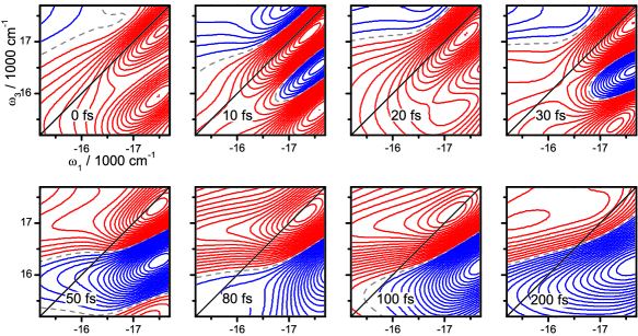
Figure 8: Simulated electronic 2D spectra of okenone, the carotenoid in LH2 M. pur. The employed values of $t_{2}$ are indicated in the panels. Line coloring follows the same conventions as described in Fig. 3

V Conclusions and Outlook

In this work we have shown that a vibronic coupling mechanism describes several central aspects of the carotenoid to BChl energy transfer dynamics, yielding moderate coupling constants $J$ close to 100 cm^-1. This value is in excellent agreement with structure-based calculations and reproduces experimental absorption spectra well. The low values of $J$ obtained from the vibronic model suffice for explaining the experimentally observed ultrafast transfer rates. This is explained by vibronic resonances, which have the potential of dramatically speeding up energy transfer. Womick2011 ; Butkus2012 ; Huelga2013 Hence, the vibronic coupling mechanism circumvents the shortcomings of Förster theory and explains static as well as dynamical properties of natural light harvesters.

The investigated carotenoid-BChl system is an extreme case of a heterodimer, meaning that donor (carotenoid) and acceptor (BChl) differ in transition energies and HR-factor. Future studies will test the vibronic coupling mechanism on energy transferring dimers where the spectroscopic properties are more alike, such as perylene bisimide dyads.Langhals2010 In such systems, both donor and acceptor show strong electron-phonon coupling, which should make vibronic effects in energy transfer dynamics even more pronounced. Another highly promising class of systems is bulk heterojunction solar cells, where vibronic coupling between donor and acceptor was recently suggested to be the mechanism behind ultrafast electron transfer.Falke2014

Appendix A Response functions

In this Appendix, the response functions used to calculated the Car 2D-spectrum are specified. The rephasing GSB term with population of $S_{2}$ and a decay due intramolecular transfer to $S_{1}$ is given as

$$R_{3g,S_{2}}(\tau_{3},\tau_{2},\tau_{1}) = \left|\mu_{S_{0}S_{2}}\right|^{4}\exp(i\omega_{S_{2}S_{0}}\tau_{1}-i\omega_{S_{2}S_{0}}\tau_{3})\exp\left(-\Gamma_{S_{2}}\tau_{1}-\Gamma_{S_{2}}\tau_{3}\right)$$ (21)

$$\exp(-g^{*}_{S_{2}S_{2}}(\tau_{1})+g^{*}_{S_{2}S_{2}}(\tau_{2})-g_{S_{2}S_{2}}(\tau_{3})$$

$$-g^{*}_{S_{2}S_{2}}(\tau_{1}+\tau_{2})-g^{*}_{S_{2}S_{2}}(\tau_{2}+\tau_{3})+g^{*}_{S_{2}S_{2}}(\tau_{1}+\tau_{2}+\tau_{3})).$$

The rephasing SE component with decay of the $S_{2}$ component due to intramolecular transfer to $S_{1}$ reads

$$R_{2g,S_{2}}(\tau_{3},\tau_{2},\tau_{1}) = \left|\mu_{S_{0}S_{2}}\right|^{4}\exp(i\omega_{S_{2}S_{0}}\tau_{1}-i\omega_{S_{2}S_{0}}\tau_{3})\exp\left(-\Gamma_{S_{2}}\tau_{1}-\Gamma_{S_{2}}\tau_{3}\right)$$ (22)

$$\exp(-g^{*}_{S_{2}S_{2}}(\tau_{1})+g_{S_{2}S_{2}}(\tau_{2})-g^{*}_{S_{2}S_{2}}(\tau_{3})$$

$$-g^{*}_{S_{2}S_{2}}(\tau_{1}+\tau_{2})-g_{S_{2}S_{2}}(\tau_{2}+\tau_{3})+g^{*}_{S_{2}S_{2}}(\tau_{1}+\tau_{2}+\tau_{3}))$$

$$\exp(-k_{S_{2}\to S_{1}}\tau_{2}).$$

For the rephasing ESA component with population transfer from $S_{2}$ to $S_{1}$ and subsequent excitation to a higher excited state one obtains

$$R^{*}_{1f,S_{2}\to S_{1}}(\tau_{3},\tau_{2},\tau_{1}) = -\left|\mu_{S_{0}S_{2}}\right|^{2}\left|\mu_{S_{1}S_{n}}\right|^{2}\exp(i\omega_{S_{2}S_{0}}\tau_{1}-i\omega_{S_{n}S_{1}}\tau_{3})\exp\left(-\Gamma_{S_{2}}\tau_{1}-\Gamma_{S_{1}}\tau_{3}\right)$$

$$\exp(-g^{*}_{S_{2}S_{2}}(\tau_{1})-g_{S_{2}S_{1}}(\tau_{2})-g_{S_{1}S_{1}}(\tau_{3})$$

$$+g^{*}_{S_{2}S_{1}}(\tau_{1}+\tau_{2})+g_{S_{2}S_{1}}(\tau_{2}+\tau_{3})-g^{*}_{S_{2}S_{1}}(\tau_{1}+\tau_{2}+\tau_{3}))$$

$$\exp(g_{S_{n}S_{2}}(\tau_{2})+2g_{S_{n}S_{1}}(\tau_{3})-g^{*}_{S_{n}S_{2}}(\tau_{1}+\tau_{2})$$

$$-g_{S_{n}S_{2}}(\tau_{2}+\tau_{3})+g^{*}_{S_{n}S_{2}}(\tau_{1}+\tau_{2}+\tau_{3})-g_{S_{n}S_{n}}(\tau_{3}))$$

$$k_{S_{2}\to S_{1}}\int_{0}^{\tau_{2}}d\tau\exp(-k_{S_{2}\to S_{1}}\tau)$$

$$\exp(2i\Im(g_{S_{2}S_{1}}(\tau_{2}-\tau)-g_{S_{1}S_{1}}(\tau_{2}-\tau)+g_{S_{1}S_{1}}(\tau_{2}-\tau+\tau_{3})-g_{S_{2}S_{1}}(\tau_{2}-\tau+\tau_{3})))$$

$$\exp(2i\Im(g_{S_{n}S_{1}}(\tau_{2}-\tau)-g_{S_{n}S_{2}}(\tau_{2}-\tau)+g_{S_{n}S_{2}}(\tau_{2}-\tau+\tau_{3})-g_{S_{n}S_{1}}(\tau_{2}-\tau+\tau_{3}))).$$

The nonrephasing response functions of GSB-, SE- and ESA-types read

$$R_{4g,S_{2}}(\tau_{3},\tau_{2},\tau_{1}) = \left|\mu_{S_{0}S_{2}}\right|^{4}\exp(-i\omega_{S_{2}S_{0}}\tau_{1}-i\omega_{S_{2}S_{0}}\tau_{3})\exp\left(-\Gamma_{S_{2}}\tau_{1}-\Gamma_{S_{2}}\tau_{3}\right)$$ (23)

$$\exp(-g_{S_{2}S_{2}}(\tau_{1})-g_{S_{2}S_{2}}(\tau_{2})-g_{S_{2}S_{2}}(\tau_{3})$$

$$+g_{S_{2}S_{2}}(\tau_{1}+\tau_{2})+g_{S_{2}S_{2}}(\tau_{2}+\tau_{3})-g_{S_{2}S_{2}}(\tau_{1}+\tau_{2}+\tau_{3})),$$

$$R_{1g,S_{2}}(\tau_{3},\tau_{2},\tau_{1}) = \left|\mu_{S_{0}S_{2}}\right|^{4}\exp(-i\omega_{S_{2}S_{0}}\tau_{1}-i\omega_{S_{2}S_{0}}\tau_{3})\exp\left(-\Gamma_{S_{2}}\tau_{1}-\Gamma_{S_{2}}\tau_{3}\right)$$ (24)

$$\exp(-g_{S_{2}S_{2}}(\tau_{1})-g^{*}_{S_{2}S_{2}}(\tau_{2})-g^{*}_{S_{2}S_{2}}(\tau_{3})$$

$$+g_{S_{2}S_{2}}(\tau_{1}+\tau_{2})+g^{*}_{S_{2}S_{2}}(\tau_{2}+\tau_{3})-g_{S_{2}S_{2}}(\tau_{1}+\tau_{2}+\tau_{3}))$$

$$\exp(-k_{S_{2}\to S_{1}}\tau_{2})$$

and

$$R^{*}_{2f,S_{2}\to S_{1}}(\tau_{3},\tau_{2},\tau_{1}) = -\left|\mu_{S_{0}S_{2}}\right|^{2}\left|\mu_{S_{1}S_{n}}\right|^{2}\exp(-i\omega_{S_{2}S_{0}}\tau_{1}-i\omega_{S_{n}S_{1}}\tau_{3})\exp\left(-\Gamma_{S_{2}}\tau_{1}-\Gamma_{S_{1}}\tau_{3}\right)$$

$$\exp(-g_{S_{2}S_{2}}(\tau_{1})+g^{*}_{S_{2}S_{1}}(\tau_{2})-g_{S_{1}S_{1}}(\tau_{3})$$

$$-g_{S_{2}S_{1}}(\tau_{1}+\tau_{2})-g^{*}_{S_{2}S_{1}}(\tau_{2}+\tau_{3})+g_{S_{2}S_{1}}(\tau_{1}+\tau_{2}+\tau_{3}))$$

$$\exp(-g^{*}_{S_{n}S_{2}}(\tau_{2})+2g_{S_{n}S_{1}}(\tau_{3})+g_{S_{n}S_{2}}(\tau_{1}+\tau_{2})$$

$$+g^{*}_{S_{n}S_{2}}(\tau_{2}+\tau_{3})-g_{S_{n}S_{2}}(\tau_{1}+\tau_{2}+\tau_{3})-g_{S_{n}S_{n}}(\tau_{3}))$$

$$k_{S_{2}\to S_{1}}\int_{0}^{\tau_{2}}d\tau\exp(-k_{S_{2}\to S_{1}}\tau)$$

$$\exp(2i\Im(g_{S_{2}S_{1}}(\tau_{2}-\tau)-g_{S_{1}S_{1}}(\tau_{2}-\tau)+g_{S_{1}S_{1}}(\tau_{2}-\tau+\tau_{3})-g_{S_{2}S_{1}}(\tau_{2}-\tau+\tau_{3})))$$

$$\exp(2i\Im(g_{S_{n}S_{1}}(\tau_{2}-\tau)-g_{S_{n}S_{2}}(\tau_{2}-\tau)+g_{S_{n}S_{2}}(\tau_{2}-\tau+\tau_{3})-g_{S_{n}S_{1}}(\tau_{2}-\tau+\tau_{3}))).$$

References

- (1) T. Renger, V. May, and O. Kuhn, Physics Reports-Review Section of Physics Letters 343, 138 (2001).
- (2) H. Lokstein and B. Grimm, eLS (John Wiley&Sons, ADDRESS, 2013).
- (3) V. Sundstrom, in Biophotonics: Spectroscopy, Imaging, Sensing, and Manipulation, NATO Science for Peace and Security Series B-Physics and Biophysics, edited by B. DiBartolo and J. Collins (PUBLISHER, ADDRESS, 2011), pp. 219–236.
- (4) R. E. Blankenship, Molecular Mechanisms of Photosynthesis, 2nd ed. (Wiley-Blackwell, Oxford, UK, 2014).
- (5) T. Polívka and V. Sundström, Chem. Rev. 104, 2021 (2004).
- (6) T. Polivka and V. Sundstrom, Chemical Physics Letters 477, 1 (2009).
- (7) T. Polivka and H. A. Frank, Accounts of Chemical Research 43, 1125 (2010).
- (8) R. S. Knox, Journal of Photochemistry and Photobiology B: Biology 49, 81 (1999).
- (9) M. Gouterman, Journal of Chemical Physics 30, 1139 (1959).
- (10) V. N. Nemykin, R. G. Hadt, R. V. Belosludov, H. Mizuseki, and Y. Kawazoe, Journal of Physical Chemistry A 111, 12901 (2007).
- (11) T. Mancal, N. Christensson, V. Lukes, F. Milota, O. Bixner, H. F. Kauffmann, and J. Hauer, Journal of Physical Chemistry Letters 3, 1497 (2012).
- (12) A. N. Macpherson, P. A. Liddell, D. Kuciauskas, D. Tatman, T. Gillbro, D. Gust, T. A. Moore, and A. L. Moore, Journal of Physical Chemistry B 106, 9424 (2002).
- (13) J. Savolainen, N. Dijkhuizen, R. Fanciulli, P. A. Liddell, D. Gust, T. A. Moore, A. L. Moore, J. Hauer, T. Buckup, M. Motzkus, and J. L. Herek, Journal of Physical Chemistry B 112, 2678 (2008).
- (14) T. H. P. Brotosudarmo, A. M. Collins, A. Gall, A. W. Roszak, A. T. Gardiner, R. E. Blankenship, and R. J. Cogdell, Biochemical Journal 440, 51 (2011).
- (15) F. Milota, C. N. Lincoln, and J. Hauer, Opt. Express 21, 15904 (2013).
- (16) N. Christensson, F. Milota, J. Hauer, J. Sperling, O. Bixner, A. Nemeth, and H. F. Kauffmann, Journal of Physical Chemistry B 115, 5383 (2011).
- (17) J. Piel, E. Riedle, L. Gundlach, R. Ernstorfer, and R. Eichberger, Optics Letters 31, 1289 (2006).
- (18) M. L. Cowan, J. P. Ogilvie, and R. J. D. Miller, Chemical Physics Letters 386, 184 (2004).
- (19) T. Brixner, T. Mancal, I. V. Stiopkin, and G. R. Fleming, Journal of Chemical Physics 121, 4221 (2004).
- (20) F. Milota, J. Sperling, A. Nemeth, and H. F. Kauffmann, Chemical Physics 357, 45 (2009).
- (21) M. J. Tauber, R. A. Mathies, X. Y. Chen, and S. E. Bradforth, Review of Scientific Instruments 74, 4958 (2003).
- (22) S. Mukamel, Principles of Nonlinear Optical Spectroscopy (Oxford University Press, New York, 1995).
- (23) J. Seibt and T. o. Pullerits, J. Chem. Phys. 141, 114106 (2014).
- (24) T. Mančal, J. Dostál, J. Pšenčík, and D. Zigmantas, Can. J. Phys. 92, 135 (2014).
- (25) T. Brixner, T. Mančal, I. V. Stiopkin, and G. R. Fleming, J. Chem. Phys. 121, 4221 (2004).
- (26) S. Tretiak, C. Middleton, V. Chernyak, and S. Mukamel, J. Phys. Chem. B 104, 9540 (2000).
- (27) V. Perlik, C. Lincoln, F. Sanda, and J. Hauer, Journal of Physical Chemistry Letters 5, 404 (2014), aa5qb Times Cited:0 Cited References Count:26.
- (28) L. D. Landau and E. Teller, Phys. Z. Sowjetunion 10, 34 (1936).
- (29) F. Sanda, Journal of Physics a-Mathematical and General 35, 5815 (2002), 584BJ Times Cited:3 Cited References Count:28.
- (30) T. Renger and R. a. Marcus, Journal of Chemical Physics 116, 9997 (2002).
- (31) J. Savolainen, R. Fanciulli, N. Dijkhuizen, A. L. Moore, J. Hauer, T. Buckup, M. Motzkus, and J. L. Herek, Proceedings of the National Academy of Sciences of the United States of America 105, 7641 (2008).
- (32) M. Z. Papiz, S. M. Prince, T. Howard, R. J. Cogdell, and N. W. Isaacs, J Mol Biol 326, 1523 (2003).
- (33) G. McDermott, S. M. Prince, A. A. Freer, A. M. Hawthornthwaite-Lawless, M. Z. Papiz, R. J. Cogdell, and N. W. Isaacs, Nature 374, 517 (1995).
- (34) P. Tavan and K. Schulten, Physical Review B 36, 4337 (1987).
- (35) L. J. Cranston, A. W. Roszak, and R. J. Cogdell, Acta Crystallographica Section F 70, 808 (2014).
- (36) D. Polli, G. Cerullo, G. Lanzani, S. De Silvestri, H. Hashimoto, and R. J. Cogdell, Biophysical Journal 90, 2486 (2006).
- (37) M. Sugisaki, M. Fujiwara, D. Kosumi, R. Fujii, M. Nango, R. J. Cogdell, and H. Hashimoto, Physical Review B 81, 245112 (2010).
- (38) G. Cerullo, G. Lanzani, M. Zavelani-Rossi, and S. De Silvestri, Physical Review B 6324, 4 (2001).
- (39) J. Hauer, H. Skenderovic, K. L. Kompa, and M. Motzkus, Chemical Physics Letters 421, 523 (2006).
- (40) R. Fujii, C. H. Chen, T. Mizoguchi, and Y. Koyama, Spectrochimica Acta Part a-Molecular and Biomolecular Spectroscopy 54, 727 (1998).
- (41) T. M. Cotton and R. P. Vanduyne, Journal of the American Chemical Society 103, 6020 (1981).
- (42) N. Christensson, F. Milota, A. Nemeth, J. Sperling, H. F. Kauffmann, T. Pullerits, and J. Hauer, Journal of Physical Chemistry B 113, 16409 (2009), times Cited: 6.
- (43) N. Christensson, F. Milota, A. Nemeth, I. Pugliesi, E. Riedle, J. Sperling, T. Pullerits, H. Kauffmann, and J. Hauer, Journal of Physical Chemistry Letters 1, 3366 (2010).
- (44) D. Kosumi, M. Komukai, H. Hashimoto, and M. Yoshizawa, Physical Review Letters 95, 213601 (2005).
- (45) D. M. Jonas, Annual Review of Physical Chemistry 54, 425 (2003).
- (46) A. Nemeth, F. Milota, T. Mancal, V. Lukes, J. Hauer, H. F. Kauffmann, and J. Sperling, Journal of Chemical Physics 132, 184514 (2010).
- (47) D. B. Turner, K. E. Wilk, P. M. G. Curmi, and G. D. Scholes, Journal of Physical Chemistry Letters 2, 1904 (2011).
- (48) V. Butkus, D. Zigmantas, L. Valkunas, and D. Abramavicius, Chemical Physics Letters 545, 40 (2012).
- (49) L. Valkunas, D. Abramavicius, and T. Mančal, Molecular Excitation Dynamics and Relaxation: Quantum Theory and Spectroscopy (WILEY-VCH Verlag, Berlin, 2013).
- (50) N. Christensson, Y. Avlasevich, A. Yartsev, K. Mullen, T. Pascher, and T. Pullerits, Journal of Chemical Physics 132, (2010).
- (51) P. O. Andersson, R. J. Cogdell, and T. Gillbro, Chemical Physics 210, 195 (1996).
- (52) H. Nagae, T. Kakitani, T. Katoh, and M. Mimuro, The Journal of Chemical Physics 98, 8012 (1993).
- (53) H. van Amerongen, L. Valkunas, and R. van Grondelle, Photosynthetic Excitons (World Scientific, Singapore, 2000).
- (54) Y. C. Cheng and R. J. Silbey, Physical Review Letters 96, 1 (2006).
- (55) A. Ishizaki and G. R. Fleming, The Journal of chemical physics 130, 234111 (2009).
- (56) N. Christensson, H. F. Kauffmann, T. o. Pullerits, and T. Mančal, The journal of physical chemistry. B 116, 7449 (2012).
- (57) V. Tiwari, W. K. Peters, and D. M. Jonas, Proceedings of the National Academy of Sciences of the United States of America 110, 1203 (2013).
- (58) a. W. Chin, J. Prior, R. Rosenbach, F. Caycedo-Soler, S. F. Huelga, and M. B. Plenio, Nature Physics 9, 113 (2013).
- (59) A. Chenu, N. Christensson, H. F. Kauffmann, and T. Mančal, Scientific reports 3, 2029 (2013).
- (60) A. Ishizaki and G. R. Fleming, The Journal of chemical physics 130, 234110 (2009).
- (61) B. P. Krueger, G. D. Scholes, and G. R. Fleming, The Journal of Physical Chemistry B 102, 5378 (1998).
- (62) D. Zigmantas, E. L. Read, T. Mancal, T. Brixner, A. T. Gardiner, R. J. Cogdell, and G. R. Fleming, Proceedings of the National Academy of Sciences of the United States of America 103, 12672 (2006).
- (63) S. Mukamel and V. Rupasov, Chemical Physics Letters 242, 17 (1995).
- (64) V. May and O. Kühn, Charge and Energy Transfer Dynamics in Molecular Systems (WILEY-VCH Verlag, Berlin, 2000).
- (65) G. D. Scholes, Annual review of physical chemistry 54, 57 (2003).
- (66) D. Beljonne, C. Curutchet, G. D. Scholes, and R. J. Silbey, 113, (2009).
- (67) J. M. Womick and A. M. Moran, Journal of Physical Chemistry B 115, 1347 (2011).
- (68) D. Polli, G. Cerullo, G. Lanzani, S. D. Silvestri, H. Hashimoto, and R. J. Cogdell, Biophys. J. 90, 2486 (2006).
- (69) N. Christensson, K. Žídek, N. C. M. Magdaong, A. M. LaFountain, H. A. Frank, and D. Zigmantas, J. Phys. Chem. B 117, 11209 (2013), pMID: 23510436.
- (70) N. Christensson, F. Milota, A. Nemeth, J. Sperling, H. F. Kauffmann, T. Pullerits, and J. Hauer, J. Phys. Chem. B 113, 16409 (2009), pMID: 19954155.
- (71) M. Sugisaki, K. Yanagi, R. Cogdell, and H. Hashimoto, Phys. Rev. B 75, 155110 (2007).
- (72) N. Christensson, T. Polivka, A. Yartsev, and T. Pullerits, Phys. Rev. B 79, 245118 (2009).
- (73) H. Cong, D. M. Niedzwiedzki, G. N. Gibson, A. M. LaFountain, R. M. Kelsh, A. T. Gardiner, R. J. Cogdell, and H. A. Frank, Journal of Physical Chemistry B 112, 10689 (2008).
- (74) S. F. Huelga and M. B. Plenio, Contemporary Physics 54, 181 (2013).
- (75) H. Langhals, A. J. Esterbauer, A. Walter, E. Riedle, and I. Pugliesi, Journal of the American Chemical Society 132, 16777 (2010).
- (76) S. M. Falke, C. A. Rozzi, D. Brida, M. Maiuri, M. Amato, E. Sommer, A. De Sio, A. Rubio, G. Cerullo, E. Molinari, and C. Lienau, Science 344, 1001 (2014).