Abstract

Abstract

If the Standard Model (SM) is an effective theory, as currently believed, it is valid up to some energy scale $\Lambda$ to which the Higgs vacuum expectation value is sensitive throughout radiative quadratic terms. The latter ones destabilize the electroweak vacuum and generate the SM hierarchy problem. For a given perturbative Ultraviolet (UV) completion, the SM cutoff can be computed in terms of fundamental parameters. If the UV mass spectrum involves several scales the cutoff is not unique and each SM sector has its own UV cutoff $\Lambda_{i}$. We have performed this calculation assuming the Minimal Supersymmetric Standard Model (MSSM) is the SM UV completion. As a result, from the SM point of view, the quadratic corrections to the Higgs mass are equivalent to finite threshold contributions. For the measured values of the top quark and Higgs masses, and depending on the values of the different cutoffs $\Lambda_{i}$, these contributions can cancel even at renormalization scales as low as multi-TeV, unlike the case of a single cutoff where the cancellation only occurs at Planckian energies, a result originally obtained by Veltman. From the MSSM point of view, the requirement of stability of the electroweak minimum under radiative corrections is incorporated into the matching conditions and provides an extra constraint on the Focus Point solution to the little hierarchy problem in the MSSM. These matching conditions can be employed for precise calculations of the Higgs sector in scenarios with heavy supersymmetric fields.

I Introduction

In the Standard Model (SM) SM as an effective field theory with a physical cutoff $\Lambda$, the Higgs mass parameter is corrected by (uncalculable) quadratic divergences that can destabilize the electroweak vacuum. This fact is usually associated with the SM hierarchy problem Gildener:1976ih . In the presence of a perturbative Ultraviolet (UV) completion (beyond the TeV scale) with heavy fields coupled to the Higgs sector, the quadratic divergences appear as finite threshold effects, which can therefore be reliably computed in perturbation theory, after the heavy states are integrated out at the matching scale between the Low-Energy (LE) and the UV High-Energy (HE) effective theories. So, if the UV completion of the SM is known and it is perturbative, the hierarchy problem is entirely due to calculable finite effects and can be fully quantified. If the UV completion is non-perturbative, as it happens in the case where the Higgs is composite, the calculation cannot rely on perturbation theory, but the presence of a new scale, even if it is dynamically generated, makes it possible to estimate the size of the threshold corrections to the Higgs mass Tavares:2013dga . Here we will consider the former case where the UV completion is perturbative.

The absence of any departure from the SM predictions in current experimental data at the LHC is pointing towards the existence of new physics at least in the multi-TeV region, by which the naturalness problem is becoming more acute. This in turn is hinting at less conventional solutions to the hierarchy problem, as e.g. hypothetical solutions provided by the theory which breaks supersymmetry at the (high) scale where supersymmetry breaking is transmitted from the hidden to the observable sector. It is therefore important to compute the large radiative contributions to the hierarchy problem in order to settle the required conditions at the high scale for the stability of the electroweak vacuum in the effective theory (the SM) below the matching scale.

In this paper we will consider the SM as the LE effective theory of the Minimal Supersymmetric Standard Model (MSSM), matching the two theories at the decoupling scale $\mathcal{Q}_{m}$ where the supersymmetric partners are integrated out. We assume the MSSM is valid up to scales of the order of the Planck scale $M_{P}$, where it can be understood as e.g. the flat limit ($M_{P}\to\infty$) of $N=1$ supergravity  Nilles:1983ge , which should eventually be in turn UV completed by some more fundamental (superstring) theory. The hope is that the fundamental theory could provide the requirements for solving the SM hierarchy problem, under the form of some HE parameter relations. For that reason, in this paper we are trying to fix the required conditions which could lead to stability of the electroweak minimum, but by no means are we trying to claim any solution to the hierarchy problem, nor even a precise quantification of the fine-tuning.

Threshold effects when matching the SM with the MSSM have been extensively studied for dimensionless parameters, as e.g. the SM Yukawa and quartic couplings, thus fixing the physical Higgs and fermion masses Draper:2013oza . For dimensional parameters, as the Higgs mass parameter, the thresholds have not been systematically considered . However, the hierarchy problem precisely resides in those dimensional parameters, as solving the equations of minimum providing the electroweak vacuum expectation value (VEV) of the Higgs field requires a certain amount of fine-tuning which quantifies the hierarchy problem .

It is thus worth improving our knowledge on the dimensional parameter thresholds. To this aim, in this paper we analyze the effects on the SM Higgs mass parameter from the decoupling of the heavy MSSM fields. This will result in precise relations to be satisfied at the matching scale $\mathcal{Q}_{m}$, in order to have the stability of the electroweak minimum. Technically, we perform the matching in the one-loop RG-improved approximation, as going beyond one-loop should not add qualitative complications or dominant contributions. Similarly we perform the matching procedure in the symmetric phase for the MSSM, so our results should be affected by tiny corrections of $\mathcal{O}(v^{2}/\mathcal{Q}_{m}^{2})$.

The outline of the paper goes as follows. In section II we present some general ideas about the decoupling using the scale invariance of the effective potential in the one-loop RG-improved approximation. We show that in the considered approximation the decoupling scale $\mathcal{Q}_{m}$ is arbitrary, although in view of minimizing (unconsidered) higher loop corrections it is convenient to take it of the order of magnitude of the masses of the decoupled fields. Simple toy models to illustrate the general matching procedure are presented in section III, where we also stress the role, for scale invariance, of the anomalous dimensions of scalar fields (included in the wave-function radiative corrections) which is an ingredient alien to the effective potential, constructed at zero external momentum. The case of the MSSM is reviewed in section IV and the detailed matching between SM and MSSM Higgs mass parameters is performed in section V. The threshold effects induced in the effective theory are computed in section VI. In particular we show that for the MSSM scenario with degenerate soft breaking masses the finite correction to the SM Higgs mass parameter precisely reproduces the result obtained by Veltman (in the context of dimensional regularization in two dimensions) Veltman:1980mj if the SM cutoff is identified with the common mass of the degenerate and heavy supersymmetric partners. Instead, for the more general scenario with non degenerate heavy masses, the effective theory can be often interpreted as a SM with different cutoffs for each (quarks, gauge bosons, …) sector. In such a case the finite correction to the SM Higgs mass parameter consists in a generalized Veltman result with deformations that can be negligible depending on the hierarchy of the spectrum. In section VII we express the HE parameters evaluated at the decoupling scale $\mathcal{Q}_{m}$ in terms of their values at the scale $\mathcal{M}$ where the supersymmetry breaking is transmitted to the observable sector, and we constrain these values to be compatible with sensible matching conditions. We then quantify the thresholds effects and their impact on the Higgs sector. We focus on the parameter region corresponding to the Focus Point (FP) solutions. The regions where the electroweak stability is not spoiled by the finite corrections in the matching conditions can be understood as a generalized FP solutions which include thresholds effects. Our conclusions are presented in section VIII, as well as a discussion on the scale, gauge and renormalization scheme dependence of our results. Finally, technical details of the calculation of the radiative corrections to the SM Higgs mass parameter stemming from the different supersymmetric sectors are presented in section A. A nice check of the consistency of our calculation is the explicit proof of the one-loop scale invariance of our results, and this is presented in section B.

II General ideas about the decoupling

Before putting forward the explicit relation of the effective potential $V$ in the LE and HE regions, let us review some general ideas about the effective potential Ford:1992mv . The effective potential improved by the RG depends, on top of the background value of fields $\phi_{i}$, on a number of running parameters $\lambda_{I}$ (they include dimensionless couplings as well as dimensionful parameters) and on the renormalization scale $\mathcal{Q}$, in such a way that the equation

$$\left[\mathcal{Q}\frac{\partial}{\partial\mathcal{Q}}+\beta_{I}\frac{\partial}{\partial\lambda_{I}}+\gamma_{i}\phi_{i}\frac{\partial}{\partial\phi_{i}}\right]V=0\$$ (1)

is fulfilled. This equation, where $\gamma_{i}$ are the anomalous dimensions of the fields $\phi_{i}$, and $\beta_{I}$ the $\beta$-functions of the parameters $\lambda_{I}$, highlights the renormalization-scale independence of the effective potential. The general solution of Eq. (1) reads as

$$V=V(\mathcal{Q}(t),\lambda_{I}(t),\phi_{i}(t))$$ (2)

where

$$\mathcal{Q}(t)=\mathcal{Q}\exp(t)\,,~{}~{}\beta_{I}(\lambda_{I}(t))=\frac{d\lambda_{I}(t)}{dt}\,,~{}~{}\gamma_{i}(\lambda_{I}(t))=\frac{d\log(\phi_{i}(t)/\phi_{i})}{dt}\,,$$ (3)

together with the boundary conditions $\lambda_{I}(0)\equiv\lambda_{I}$, $\phi_{i}(0)\equiv\phi_{i}$.

In practice the scale independence of the effective potential (2) holds up to the level of perturbation theory where the potential is computed. In particular if we make a loop expansion of the operator $V$ as

$$V=\sum_{\ell\geq 0}V^{(\ell)}\ ,$$ (4)

the RG-improved potential $V^{(0)}$ has a very strong scale dependence. This dependence is reduced by considering $V^{(0)}+V^{(1)}$, where $V^{(1)}$ includes the terms that correspond to the field redefinitions $\phi_{i}(t)\equiv(1+Z_{i}^{(1)}(t))\phi_{i}$, and the one-loop RG-improved Coleman-Weinberg contribution $\Delta V^{(1)}$. In fact, in $V^{(0)}+V^{(1)}$ the whole one-loop scale dependence cancels out and different choices of $Q$ only affect higher order corrections. Whereas the explicit expression of $Z_{i}(t)$ depends on the specific model, the contribution $\Delta V^{(1)}$ can be generically written as Coleman:1973jx  

$$\Delta V^{(1)}=\frac{1}{64\pi^{2}}STr\mathcal{M}^{4}(\phi_{i})\left[\log\frac{\mathcal{M}^{2}(\phi_{i})}{\mathcal{Q}^{2}}-\mathcal{C}\right]\$$ (5)

where $STr$ includes the number of degrees of freedom of the different mass eigenstates as well as a negative sign for fermions.

The electroweak-breaking condition, described as the solution to the equations of minimum

$$\frac{\partial V}{\partial\phi_{i}}=0\ ,$$ (6)

is also scale independent. Such condition can thus be deduced from the potential $V$ at any scale $\mathcal{Q}$ and any loop order. However since one is only able to compute $\Delta V^{(\ell)}$ and $Z_{i}^{(\ell)}$ with $\ell\leq n$ (i.e. up to some perturbative order $n$), and the minimization condition should eventually be related to electroweak observables, in practical cases it is advisable to minimize $\sum_{\ell\leq n}V^{(\ell)}$ (with scale dependence at $n+1$ loop order) at the electroweak scale $\mathcal{Q}=\mathcal{Q}_{EW}$. Employing this choice of renormalization scale is subtle when also heavy fields are involved, as we describe now.

We consider a HE theory with light and heavy fields. Light fields have electroweak-breaking and/or invariant masses of order (or below) $\mathcal{Q}_{EW}$, whereas heavy fields have masses $M\gg\mathcal{Q}_{EW}$. To any fixed order in the loop expansion heavy fields can induce large logarithms in the minimization condition evaluated at $\mathcal{Q}=\mathcal{Q}_{EW}$ Bando:1992wy . For this reason, the minimization should still be performed at $\mathcal{Q}=\mathcal{Q}_{EW}$, but in the LE effective theory where the heavy fields have been decoupled.

As we are considering mass-independent renormalization schemes the decoupling of heavy fields has to be performed at some scale $\mathcal{Q}_{m}$. In such a case the effective description at $\mathcal{Q}\ll\mathcal{Q}_{m}$ is obtained in two steps: i) Matching at $\mathcal{Q}=\mathcal{Q}_{m}$ of the HE Lagrangian to an effective Lagrangian (which has all light-fields interactions allowed by the HE symmetry), and ii) Running of the effective couplings from $\mathcal{Q}_{m}$ to $\mathcal{Q}_{EW}$. The matching of the couplings of the light scalar sector can be obtained by exploiting the LE and HE effective potentials.

By construction, the HE and LE theories (in the presence of only light-field backgrounds) have the same RG-improved potentials at the decoupling scale, i.e. $V_{LE}(\mathcal{Q}_{m})=V(\mathcal{Q}_{m})$ (LE quantities carry a “$LE$” subscript; for HE quantities the subscript “$HE$” is suppressed). In the ideal case of perfect scale invariance this equivalence is true at any scale, and the choice of $\mathcal{Q}_{m}$ at which one matches the two potentials is fully arbitrary. However, in realistic situations where the potentials are calculated at a given loop approximation, $\mathcal{Q}_{m}$ has to be set at a value that presumably minimizes the unknown higher order corrections coming from heavy fields. This motivates the choice $\mathcal{Q}_{m}\sim M$.

The decoupling procedure involves some technical details when applied to realistic frameworks. The first issue arises when the HE theory contains several Higgses acquiring VEVs. This complication does not lead to any difficulties in our analysis as we are considering scenarios with the SM as an effective description. In fact we are restricting ourselves to cases where all the multi-Higgs VEVs in the interaction-eigenstate basis can be aligned along a unique VEV in the mass-eigenstate basis (and this direction corresponds to the light Higgs of the SM). Clearly this is possible because we are assuming the mass of the extra-Higgses to be $M\gg\mathcal{Q}_{EW}$. A second issue arises when there are several heavy fields with masses $M_{I}$. If they differ by orders of magnitude, there exists no choice of $\mathcal{Q}_{m}$ that avoids large logarithms in the matching conditions. In this case the decoupling procedure has to be repeated as many times as the number of hierarchically different heavy mass thresholds. Of course when all $M_{I}$ are similar, the decoupling can be performed just once with $\mathcal{Q}_{m}$ fixed at some intermediate value among $M_{I}$. The simplified concrete examples of the next sections will better clarify the details of the decoupling procedure.

III Decoupling in some toy models

In this section we illustrate the previous ideas about decoupling. We first analyze a toy model with only one heavy degree of freedom. Second we consider a case with several scalar heavy particles and light fermions which contribute to the light scalar wave function renormalization. The reader not interested in those technical details can jump straightforwardly to section IV.

III.1 First toy model: scalars

We consider a toy model consisting of a light scalar $\phi$ and a heavy scalar $S$ with a HE Lagrangian

$$\mathcal{L}=-\Omega+\frac{1}{2}(\partial\phi)^{2}+\frac{1}{2}(\partial S)^{2}-\frac{1}{2}m^{2}\phi^{2}-\frac{1}{4!}\lambda\phi^{4}-\frac{1}{2}M^{2}S^{2}-\frac{1}{2}h^{2}\phi^{2}S^{2}$$ (7)

where for simplicity the quartic coupling of the $S$ field has been set to zero, although it is not protected by any symmetry. After decoupling the $S$-field the theory is described by the effective Lagrangian

$$\mathcal{L}_{LE}=-\Omega_{LE}+\frac{1}{2}(\partial\phi_{LE})^{2}-\frac{1}{2}m_{LE}^{2}\phi_{LE}^{2}-\frac{1}{4!}\lambda_{LE}\phi_{LE}^{4}~{}.$$ (8)

In both Lagrangians the parameters are running with the scale $\mathcal{Q}$.

Since $S$ does not acquire a VEV, the electroweak breaking field $\phi$ is aligned to $\phi_{LE}$. The tree-level (RG-improved) matching of the parameters at the scale $\mathcal{Q}_{m}$ is then trivial:

$$\Omega_{LE}(\mathcal{Q}_{m})=\Omega(\mathcal{Q}_{m}),\ \phi_{LE}(\mathcal{Q}_{m})=\phi(\mathcal{Q}_{m}),\ m_{LE}(\mathcal{Q}_{m})=m(\mathcal{Q}_{m}),\ \lambda_{LE}(\mathcal{Q}_{m})=\lambda(\mathcal{Q}_{m}).$$ (9)

At this point one could already run the LE parameters from $\mathcal{Q}_{m}$ to $\mathcal{Q}_{EW}$ and obtain the minimization condition. However the result would strongly depend on the choice of $\mathcal{Q}_{m}$. Indeed, since the LE and HE parameters run very differently, one would obtain different minimization conditions for different values of $\mathcal{Q}_{m}$ in Eq. (9), even though the fundamental HE parameters would be kept fixed. This problem is alleviated by performing a one-loop matching. Hereafter we adopt the $\overline{\rm MS}$ renormalization scheme to subtract the one-loop divergences.

In the present model there is no one-loop wave function renormalization and the tree level relation $\phi_{LE}(\mathcal{Q}_{m})=\phi(\mathcal{Q}_{m})$ is preserved at one loop. The one-loop matching of the other parameters can be obtained by matching the LE and the HE effective potentials where all parameters are at the scale $\mathcal{Q}_{m}$. We thus impose the relation

$$V(\phi)=V_{LE}(\phi)\,$$ (10)

with

$$V(\phi) = \Omega+\frac{1}{2}m^{2}\phi^{2}+\frac{1}{4!}\lambda\phi^{4}+\frac{1}{64\pi^{2}}\sum_{i=\phi,S}m_{i}^{4}\left(\log\frac{m_{i}^{2}}{\mathcal{Q}_{m}^{2}}-\frac{3}{2}\right)\,,$$ (11)

$$V_{LE}(\phi) = \Omega_{LE}+\frac{1}{2}m_{LE}^{2}\phi^{2}+\frac{1}{4!}\lambda_{LE}\phi^{4}+\frac{1}{64\pi^{2}}m_{\phi_{LE}}^{4}\left(\log\frac{m_{\phi_{LE}}^{2}}{\mathcal{Q}_{m}^{2}}-\frac{3}{2}\right)+\mathcal{O}(\phi^{6}/M^{2})\,,$$

where $m_{\phi}^{2}=m^{2}+\frac{1}{2}\lambda\phi^{2}$, $m_{S}^{2}=M^{2}+h^{2}\phi^{2}$ and $m_{\phi_{LE}}^{2}=m_{LE}^{2}+\frac{1}{2}\lambda_{LE}\phi^{2}$. This matching leads to

$$\Omega_{LE}(\mathcal{Q}_{m}) =\left[\Omega(\mathcal{Q}_{m})+\frac{M^{4}}{64\pi^{2}}\log\frac{M^{2}}{\mathcal{Q}_{m}^{2}}\right]-\frac{3M^{4}}{128\pi^{2}}~{},$$

$$m_{LE}^{2}(\mathcal{Q}_{m}) =\left[m^{2}(\mathcal{Q}_{m})+\frac{h^{2}M^{2}}{16\pi^{2}}\log\frac{M^{2}}{\mathcal{Q}_{m}^{2}}\right]-\frac{h^{2}M^{2}}{16\pi^{2}}~{},$$ (12)

$$\lambda_{LE}(\mathcal{Q}_{m}) =\left[\lambda(\mathcal{Q}_{m})+\frac{12}{32\pi^{2}}h^{4}\log\frac{M^{2}}{\mathcal{Q}_{m}^{2}}\right]~{},$$

which holds up to two-loop corrections  and where all parameters are evaluated at the scale $\mathcal{Q}_{m}$. In particular due to the one-loop scale invariance of the HE and LE effective potentials, the arbitrariness of $\mathcal{Q}_{m}$ in (III.1) is guaranteed at one-loop level. In fact, within each parenthesis in (III.1) the logarithms compensate the one-loop running of the parameters whose evolutions are given by the $\beta$-functions

$$\beta_{\Omega_{LE}} =\frac{1}{32\pi^{2}}m_{LE}^{4},\quad\beta_{\Omega}=\frac{1}{32\pi^{2}}(m^{4}+M^{4})\ ,$$

$$\beta_{m_{LE}^{2}} =\frac{1}{8\pi^{2}}\lambda_{LE}m_{LE}^{2},\quad\beta_{m^{2}}=\frac{1}{8\pi^{2}}(\lambda m^{2}+h^{2}M^{2})\ ,$$ (13)

$$\beta_{\lambda_{LE}} =\frac{6}{32\pi^{2}}\lambda_{LE}^{2},\quad\beta_{\lambda}=\frac{6}{32\pi^{2}}(\lambda^{2}+4h^{4})\ .$$

This shows that in the one-loop approximation the running and matching procedures are commutative and the LE theory is independent of the decoupling scale.

The one-loop freedom in the choice of $\mathcal{Q}_{m}$ can be used to minimize the higher order corrections to (III.1). To this aim it is sensible to choose $\mathcal{Q}_{m}=M$. In this particular case the matching for $m_{LE}^{2}$ turns out to be

$$m_{LE}^{2}(M)=m^{2}(M)-\frac{h^{2}}{16\pi^{2}}\,M^{2}\ .$$ (14)

The second term is the large threshold correction that, in a more realistic theory as the SM, would destabilize the electroweak vacuum and would introduce a hierarchy problem.

III.2 Second toy model: scalars and fermions

Further subtleties of the decoupling procedure can be described in a slightly more complicated scenario. We consider a HE theory consisting of a light real scalar $\phi$, a light Dirac fermion $\Psi$, and a number of heavy scalars $S_{I}$ with masses $M_{I}$ of similar magnitude:

$$\mathcal{L}=-\Omega+\frac{1}{2}(\partial\phi)^{2}-\frac{m^{2}}{2}\phi^{2}-\frac{\lambda}{4!}\phi^{4}+\frac{1}{2}\sum_{I}\left[(\partial S_{I})^{2}-(M_{I}^{2}+h_{I}^{2}\phi^{2})S_{I}^{2}\right]+i\bar{\Psi}\not{\partial}\Psi-Y\phi\bar{\Psi}\Psi~{}.$$ (15)

This theory can be described at LE by

$$\mathcal{L}_{LE}=-\Omega_{LE}+\frac{1}{2}(\partial\phi_{LE})^{2}-\frac{m_{LE}^{2}}{2}\phi_{LE}^{2}-\frac{\lambda_{LE}}{4!}\phi_{LE}^{4}+i\bar{\Psi}_{LE}\,\not{\partial}\Psi_{LE}-Y_{LE}\phi_{LE}\bar{\Psi}_{LE}\,\Psi_{LE}$$ (16)

and the dependence with respect to $\mathcal{Q}$ is implicit in Eqs. (15) and (16).

Since the $S_{I}$ fields do not acquire any VEV and their integration do not lead to any tree-level correction to the LE couplings, the tree-level matching is trivial. Instead the one-loop matching is less straightforward due, for instance, to the radiative corrections to the kinetic terms. As we are interested in the one-loop electroweak-breaking conditions, we will focus on the effective potential of the light scalar field. In particular we want to calculate the RG-improved one-loop matching at the scale $\mathcal{Q}_{m}$. To this aim we first run all parameters in (15) and (16) to $\mathcal{Q}_{m}$, and then we evaluate the LE and HE one-loop potentials. We thus absorb the kinetic-term radiative corrections  $(1-2Z_{\phi}(\mathcal{Q}_{m}))$ and $(1-2Z_{\phi_{LE}}(\mathcal{Q}_{m}))$ into field redefinitions of $\phi$ and $\phi_{LE}$ respectively, where $d[Z_{i}(\mathcal{Q})]/d\log\mathcal{Q}=\gamma_{i}(\mathcal{Q})$, the anomalous dimension at one-loop order. The expansion of the HE RG-improved one-loop potential at the scale ${\mathcal{Q}_{m}}$ has to reproduce the LE one at the same scale. We hence impose the matching

$$V(\phi)=V_{LE}(\phi)\,$$ (17)

with

$$V(\phi) = \Omega+\frac{1}{2}m^{2}(1+2Z_{\phi})\phi^{2}+\frac{1}{4!}\lambda(1+4Z_{\phi})\phi^{4}+\sum_{i=\phi,S_{I},\Psi}n_{i}\frac{m_{i}^{4}}{64\pi^{2}}\left(\log\frac{m_{i}^{2}}{\mathcal{Q}_{m}^{2}}-\frac{3}{2}\right)\,,$$

$$V_{LE}(\phi_{LE}) = \Omega_{LE}+\frac{1}{2}m_{LE}^{2}(1+2Z_{\phi_{LE}})\phi_{LE}^{2}+\frac{1}{4!}\lambda_{LE}(1+4Z_{\phi_{LE}})\phi_{LE}^{4}$$

$$+ \sum_{i=\phi_{LE},\Psi_{LE}}n_{i}\frac{m_{i}^{4}}{64\pi^{2}}\left(\log\frac{m_{i}^{2}}{\mathcal{Q}_{m}^{2}}-\frac{3}{2}\right)+\mathcal{O}(\phi_{LE}^{6}/M^{2})\,,$$

where $m_{\phi}^{2}=m^{2}+\frac{1}{2}\lambda\phi^{2}$, $m_{S_{I}}^{2}=M_{I}^{2}+h^{2}\phi^{2}$, $m_{\Psi}^{2}=Y^{2}\phi^{2}$, $m_{\phi_{LE}}^{2}=m_{LE}^{2}+\frac{1}{2}\lambda_{LE}\phi_{LE}^{2}$, $m_{\Psi_{LE}}^{2}=Y_{LE}^{2}\phi_{LE}^{2}$, and $n_{i}=1(-4)$ for real bosons (Dirac fermions). This implies

$$\Omega_{LE}(\mathcal{Q}_{m}) =\left[\Omega(\mathcal{Q}_{m})+\sum_{I}\frac{M_{I}^{4}}{64\pi^{2}}\log\frac{M_{I}^{2}}{\mathcal{Q}_{m}^{2}}\right]-\sum_{I}\frac{3M_{I}^{4}}{128\pi^{2}}~{},$$

$$m_{LE}^{2}(\mathcal{Q}_{m}) =\left[m^{2}(\mathcal{Q}_{m})[1+2Z_{\phi}(\mathcal{Q}_{m})-2Z_{\phi_{LE}}(\mathcal{Q}_{m})]+\sum_{I}\frac{h_{I}^{2}M_{I}^{2}}{16\pi^{2}}\log\frac{M_{I}^{2}}{\mathcal{Q}_{m}^{2}}\right]-\sum_{I}\frac{h_{I}^{2}M_{I}^{2}}{16\pi^{2}}~{},$$

$$\lambda_{LE}(\mathcal{Q}_{m}) =\lambda(\mathcal{Q}_{m})[1+4Z_{\phi}(\mathcal{Q}_{m})-4Z_{\phi_{LE}}(\mathcal{Q}_{m})]+\sum_{I}\frac{12h_{I}^{4}}{32\pi^{2}}\log\frac{M_{I}^{2}}{\mathcal{Q}_{m}^{2}}~{}.$$ (18)

where we are using the tree-level matching condition $Y_{LE}(\mathcal{Q}_{m})=Y(\mathcal{Q}_{m})$ .

In this toy model only light degrees of freedom generate $Z_{\phi}$ and $Z_{\phi_{LE}}$ at one loop via couplings that have trivial tree-level matching: it thus follows that $Z_{\phi}=Z_{\phi_{LE}}$ . Moreover, in view of minimizing higher loop corrections in the matching of $m_{LE}^{2}$, one can adopt the choice $\mathcal{Q}_{m}=\bar{M}$, where $\bar{M}$ is defined as

$$\log\bar{M}^{2}=\frac{\sum_{I}h_{I}^{2}M_{I}^{2}\log(M_{I}^{2})}{\sum_{I}h_{I}^{2}M_{I}^{2}}\,,$$ (19)

so that only the non-logarithmic one-loop contribution is left in the matching condition for $m_{LE}^{2}$:

$$m_{LE}^{2}(\bar{M})=m^{2}(\bar{M})-\sum_{I}\frac{h_{I}^{2}}{16\pi^{2}}\,M_{I}^{2}~{}.$$ (20)

Of course the choice (19) is expected to reduce the higher order correction in the $m_{LE}^{2}$ matching only if the relation $\log\bar{M}^{2}\sim\log M_{I}^{2}$ occurs for all $I$’s. Otherwise, as already stressed in section II, it is worth reiterating the decoupling procedure at each mass scale $M_{I}$.

IV The SM/MSSM matching

In this section we use the MSSM one-loop RG-improved effective potential to determine the radiative corrections that can destabilize the electroweak breaking condition in such a model. The Higgs sector contains two doublets $H_{1}$ and $H_{2}$ where in our convention $H_{2}$ gives the mass to the top quark and $H_{1}$ to the bottom quark and tau lepton. The MSSM Higgs Lagrangian, including only the one-loop wave function renormalization for the Higgs doublets $Z_{h_{i}}$, can be written as

$$\mathcal{L}_{MSSM}=\sum_{i}(1-2Z_{h_{i}})|D_{\mu}H_{i}|^{2}-V(H_{1},H_{2})$$ (21)

where $V(H_{1},H_{2})$ is the tree-level MSSM Higgs potential. Then the one-loop RG-improved MSSM potential of the neutral Higgs fields $h_{i}=\textrm{Re}H_{i}^{0}$ ($i=1,2$) is

$$V(h_{1},h_{2}) = m_{1}^{2}(1+2Z_{h_{1}})h_{1}^{2}+m_{2}^{2}(1+2Z_{h_{2}})h_{2}^{2}-2m_{3}^{2}h_{1}h_{2}(1+Z_{h_{1}}+Z_{h_{2}})$$ (22)

$$+ \frac{g_{Z}^{2}}{2}[h_{1}^{2}(1+2Z_{h_{2}})-h_{2}^{2}(1+2Z_{h_{2}})]^{2}+\Delta V_{MSSM}(h_{1},h_{2})\ ,$$

where $\Delta V_{MSSM}$ is the Coleman-Weinberg contribution generated by all fields of the MSSM and 

$$g_{Z}^{2}\equiv(g_{Y}^{2}+g_{2}^{2})/4,\quad m_{1}^{2}\equiv m_{H_{1}}^{2}+\mu^{2},\quad m_{2}^{2}\equiv m_{H_{2}}^{2}+\mu^{2}.$$ (23)

The above equation is understood at an arbitrary renormalization scale $\mathcal{Q}$.

In view of the strong LHC bounds on the masses of supersymmetric particles we match the MSSM with the SM at some high scale $\mathcal{Q}_{m}$, say (multi-)TeV. To this aim we employ the effective potential techniques adopted in the previous examples. For simplicity, we assume all parameters to be real although the extension to cases with complex parameters (and $CP$ violation) is straightforward.

Contrarily to the previous examples, the MSSM has two fields, in the gauge eigenstate basis, that acquire VEVs. We then go to the mass eigenstate basis to work out the matching (first at the tree-level, then at one-loop). The field rotation can be performed by neglecting the $\mathcal{O}(v^{2}/\mathcal{Q}_{m}^{2})$ electroweak-breaking contributions (i.e. we proceed in the electroweak symmetry unbroken phase) since the $CP$-odd Higgs mass $m_{A}$ is assumed to be much heavier than the electroweak scale. The resulting potential can be matched to the SM potential whose one-loop RG-improved expression is given by

$$V_{LE}(h_{LE})=-m_{LE}^{2}(1+2Z_{h_{LE}})h_{LE}^{2}+\frac{\lambda_{LE}}{2}(1+4Z_{h_{LE}})h_{LE}^{4}+\Delta V_{SM}(h_{LE})~{},$$ (24)

where $\Delta V_{SM}$ is the SM one-loop RG-improved Coleman-Weinberg potential in the presence of the background field $h_{LE}=\textrm{Re}\,H_{LE}^{0}$ (with $H_{LE}$ being the SM Higgs doublet). In Eq. (24) and hereafter the effective higher-order operators, which are small due the large hierarchy between heavy and light fields, are neglected.

IV.1 Tree-level matching

In order to derive the RG-improved tree-level matching we will focus on the quadratic part of the tree-level MSSM potential, $V^{(0)}(h_{1},h_{2})$, which can be extracted from (22). At the matching scale $\mathcal{Q}_{m}$ we thus obtain

$$V^{(0)}(h_{1},h_{2}) = m_{1}^{2}h_{1}^{2}+m_{2}^{2}h_{2}^{2}-2m_{3}^{2}h_{1}h_{2}+\frac{g_{Z}^{2}}{2}(h_{1}^{2}-h_{2}^{2})^{2}\ .$$ (25)

The potential $V^{(0)}(h_{1},h_{2})$ at $\mathcal{Q}_{m}$ can be rewritten in the mass eigenstate basis as

$$V^{(0)}(h,H)=-m^{2}h^{2}+m_{H}^{2}H^{2}+\cdots\$$ (26)

with $m^{2}\ll m_{H}^{2}=m_{1}^{2}+m_{2}^{2}+m^{2}$. This field transformation is achieved by the rotation

$$\left(\begin{matrix}h_{1}\\ h_{2}\end{matrix}\right)=R_{\beta}\left(\begin{matrix}h\\ H\end{matrix}\right)\ ,\quad R_{\beta}=\left(\begin{matrix}\cos\beta&-\sin\beta\\ \sin\beta&\cos\beta\end{matrix}\right)$$ (27)

such that

$$(h_{1},h_{2})\left(\begin{matrix}m_{1}^{2}&-m_{3}^{2}\\ -m_{3}^{2}&m_{2}^{2}\end{matrix}\right)\left(\begin{matrix}h_{1}\\ h_{2}\end{matrix}\right)=(h,H)\left(\begin{matrix}-m^{2}&0\\ 0&m^{2}_{H}\end{matrix}\right)\left(\begin{matrix}h\\ H\end{matrix}\right)\ .$$ (28)

Note that Eqs. (27) and (28) are equivalent to require

$$m_{3}^{4} =(m_{1}^{2}+m^{2})(m_{2}^{2}+m^{2})~{},$$ (29)

$$\tan 2\beta =\frac{2m_{3}^{2}}{m_{2}^{2}-m_{1}^{2}}$$ (30)

or, alternatively

$$m_{2}^{2} =m_{3}^{2}/\tan\beta-m^{2}~{},$$

$$m_{1}^{2} =m_{3}^{2}\tan\beta-m^{2}~{},$$ (31)

with $\tan\beta\geq 1$, as we are assuming $m_{3}^{2}>0$ and $m_{1}^{2}\geq m_{2}^{2}$. In particular since we are in the decoupling limit $m^{2}\ll m_{H}^{2}$, our definition of $\tan\beta$ coincides with the MSSM one, $\tan\beta=v_{2}/v_{1}$ where $v_{i}\equiv\langle h_{i}\rangle$. Combining the above relations we also have the explicit expression for the light mass eigenstate

$$m^{2} = -m_{1}^{2}\cos^{2}\beta-m_{2}^{2}\sin^{2}\beta+m_{3}^{2}\sin 2\beta~{}.$$ (32)

In the mass eigenstate basis $(h,H)$ it is easy to obtain the tree-level matching to the SM. If one extracts the $V^{(0)}_{LE}(h_{LE})$ part from the LE one-loop potential of $h_{LE}$, Eq. (24), and matches it to $V^{(0)}(h,H)$ at $\mathcal{Q}_{m}$, one obtains

$$h_{LE}(\mathcal{Q}_{m})=h(\mathcal{Q}_{m}),\ m_{LE}(\mathcal{Q}_{m})=m(\mathcal{Q}_{m}),\ \lambda_{LE}(\mathcal{Q}_{m})=g_{Z}^{2}(\mathcal{Q}_{m})\cos^{2}2\beta~{}\ {\rm[tree~{}level]}\ .$$ (33)

Similarly the matching of the LE and HE Yukawa interactions at $\mathcal{Q}_{m}$ yields

$$y_{t}(\mathcal{Q}_{m})=Y_{t}(\mathcal{Q}_{m})\sin\beta\ ,\quad y_{b,\tau}(\mathcal{Q}_{m})=Y_{b,\tau}(\mathcal{Q}_{m})\cos\beta~{},\qquad{\rm[tree~{}level]}\$$ (34)

where $y_{t,\tau,b}$ and $Y_{t,\tau,b}$ are respectively the top quark, tau lepton and bottom quark Yukawa couplings in the SM and in the MSSM.

Of course there might already be a problem at tree level: the right hand side of Eq. (32) is a linear combination of potentially large masses squared while the left hand side is a mass squared which is required to be at the electroweak scale. This fine-tuning is essentially equivalent to that in Eq. (29). This is the main naturalness problem in the MSSM. This problem cannot be tackled unless we know the (fundamental) theory responsible for triggering supersymmetry breaking at the high scale $\mathcal{M}$ in the hidden sector and dictating the size of the supersymmetry breaking parameters in the observable sector. The FP solution Feng:1999zg ; Delgado:2014vha just uncovers the functional relationships between fundamental parameters at the high scale $\mathcal{M}$ for which the naturalness problem is circumvented. However even if we accept that the fundamental theory might provide a solution to the tree-level stability we still have to worry for loop corrections, e.g. in the effective theory as those computed in Ref. Veltman:1980mj . The matching including one loop corrections will be done in the next section.

IV.2 One-loop level matching

We now proceed with the one-loop matching. Again we want to work in the mass eigenstate basis. We then impose the tree-level matching conditions (31) in the one-loop term $\Delta V_{MSSM}$ of (22), and expand $\Delta V_{MSSM}$. Such expansion produces some new quadratic contributions that we absorb as

$$V(h_{1},h_{2})=\widetilde{m}_{1}^{2}h_{1}^{2}+\widetilde{m}_{2}^{2}h_{2}^{2}-2\widetilde{m}_{3}^{2}h_{1}h_{2}+\cdots$$ (35)

where

$$\widetilde{m}_{i}^{2}=m_{i}^{2}+2Z_{h_{i}}m_{i}^{2}+\Delta m_{i}^{2}~{},\qquad \Delta m_{i}^{2}=\left.\frac{\partial\Delta V_{{MSSM}}}{\partial h_{i}^{2}}\right|_{h_{i}=0}~{},$$ (36)

$$\widetilde{m}_{3}^{2}=m_{3}^{2}+(Z_{h_{1}}+Z_{h_{2}})m_{3}^{2}+\Delta m_{3}^{2}~{},\qquad \Delta m_{3}^{2}=-\frac{1}{2}\left.\frac{\partial\Delta V_{{MSSM}}}{\partial h_{1}h_{2}}\right|_{h_{i}=0}~{},$$

with $i=1,2$. As previously done for the tree-level matching, we diagonalize the quadratic potential (35) by a rotation $R_{\beta}$ (whose angle differs from that of section IV.1 although for notational simplicity we are keeping the same notation for both) leading to a light mass eigenstate $h$ with squared mass $-\widetilde{m}^{2}$ and a heavy eigenstate $H$ with squared mass $\widetilde{m}_{H}^{2}=\widetilde{m}_{1}^{2}+\widetilde{m}_{2}^{2}+\widetilde{m}^{2}$, where

$$\widetilde{m}^{2} = m^{2}+2m^{2}Z_{h}+\Delta m^{2}\,,$$

$$m^{2} = -m_{1}^{2}\cos^{2}\beta-m_{2}^{2}\sin^{2}\beta+m_{3}^{2}\sin 2\beta\,,$$ (37)

$$\Delta m^{2} = -\Delta m_{1}^{2}\cos^{2}\beta-\Delta m_{2}^{2}\sin^{2}\beta+\Delta m_{3}^{2}\sin 2\beta~{},$$

and $Z_{h}\equiv\cos^{2}\beta Z_{h_{1}}+\sin^{2}\beta Z_{h_{2}}$ is the wave function renormalization in the MSSM for the mass eigenstate $h$ . This diagonalization requires

$$\widetilde{m}_{2}^{2} =\widetilde{m}_{3}^{2}/\tan\beta-\widetilde{m}^{2}~{},$$

$$\widetilde{m}_{1}^{2} =\widetilde{m}_{3}^{2}\tan\beta-\widetilde{m}^{2}\ ,$$ (38)

which can be used to express, as it is customary in the MSSM, $\tan\beta$ and the lightest eigenvalue $-\widetilde{m}^{2}$ as functions of the fundamental parameters:

$$\widetilde{m}^{2} = -\widetilde{m}_{1}^{2}\cos^{2}\beta-\widetilde{m}_{2}^{2}\sin^{2}\beta+\widetilde{m}_{3}^{2}\sin 2\beta\ ,$$ (39)

$$\tan 2\beta=\frac{2\,\widetilde{m}_{3}^{2}}{\widetilde{m}_{2}^{2}-\widetilde{m}_{1}^{2}}\ .$$

In order to perform the complete one-loop matching, we would need to consider $\Delta V_{SM}$. As the light (i.e. SM) fields provide the same contributions to $\Delta V_{SM}$ and $\Delta V_{MSSM}$ modulo the tree-level matching of Yukawa couplings in Eq. (34) (cf. also section V), we can proceed by taking into account only the heavy non-SM fields in $\Delta m_{1}^{2}$, $\Delta m_{2}^{2}$ and $\Delta m_{3}^{2}$. Then the one-loop RG-improved matching of the quadratic term in the HE and LE theories turns out to be

$$m^{2}_{LE}(\mathcal{Q}_{m}) = m^{2}(\mathcal{Q}_{m})(1+2\Delta Z_{h}(\mathcal{Q}_{m}))+\Delta m^{2}(\mathcal{Q}_{m})~{},$$ (40)

where

$$\Delta Z_{h}(\mathcal{Q}_{m}) = Z_{h}(\mathcal{Q}_{m})-Z_{h_{LE}}(\mathcal{Q}_{m})~{}.$$ (41)

We hence stress that the requirement $m^{2}(\mathcal{Q}_{m})\sim\mathcal{Q}^{2}_{EW}$ is not sufficient to guarantee sensible electroweak breaking conditions as these could be destabilized by $\Delta m^{2}$ and $\Delta Z_{h}$.

V $\Delta m^{2}$ in the MSSM with high susy-breaking scale

We will now explain the main lines to determine $\Delta m^{2}$. We remind that all the MSSM particles, except the SM ones, are assumed to be heavy. The one-loop potential $\Delta V_{MSSM}(h_{1},h_{2})$ can be split into two separated terms: one term contains contributions from the Higgs sector $A,H,H^{\pm}$ and the SM fields, and the second one does it from the field superpartners $\tilde{f}$ (with $\tilde{f}$ representing the whole list of squarks, sleptons, charginos and neutralinos). Due to the triviality of the tree-level matching conditions (33) and (34), it is easy to see as we already noticed that the light fields provide the same contribution to $\Delta V_{MSSM}(h)$ and to $\Delta V_{SM}(h_{LE})$. Because of this property the correction $\Delta m^{2}$ can be calculated as in Eq. (IV.2) with

$$\Delta m_{I}^{2} = \sum_{r=\tilde{f},A,H,H^{\pm}}\Delta m_{I,r}^{2}\,,$$ (42)

$$\Delta m_{i,r}^{2}=\left.\frac{\partial\Delta V_{{MSSM,r}}}{\partial h_{i}^{2}}\right|_{h_{i}=0} \Delta m_{3,r}^{2}=\left.-\frac{1}{2}\frac{\partial\Delta V_{{MSSM,r}}}{\partial h_{1}h_{2}}\right|_{h_{i}=0}~{},$$ (43)

where $I=(i,3)$, $i=1,2$ and $\Delta V_{MSSM,r}$ is the MSSM one-loop potential generated by the field $r$.

The explicit form of $\Delta m_{I,r}^{2}$ depends on the renormalization scheme. In the $\overline{\rm MS}$ scheme (or equivalently at this level $\overline{\rm DR}$), for which $\mathcal{C}=(3/2){\bf 1}$ in Eq. (5) for scalars and fermions, it results

$$\Delta m_{i,r}^{2}=\left.\frac{n_{r}}{32\pi^{2}}\frac{\partial m_{r}^{2}}{\partial h_{i}^{2}}G(m_{r}^{2})\right|_{h_{i}=0}\ ,\,\,\,\,\,\Delta m_{3,r}^{2}=\left.-\frac{n_{r}}{64\pi^{2}}\frac{\partial m_{r}^{2}}{\partial h_{1}h_{2}}G(m_{r}^{2})\right|_{h_{i}=0}~{},$$ (44)

where $n_{r}$ stands for the number of degrees of freedom of the particle $r$ and is positive (negative) for bosons (fermions), while the function $G(x^{2})$ is defined as

$$G(x^{2})\equiv x^{2}\left(\log\frac{x^{2}}{\mathcal{Q}_{m}^{2}}-1\right)\,.$$ (45)

For simplicity we determine $\Delta m^{2}$ by neglecting the corrections coming from first and second generations of squarks and sleptons (the expressions are however fully general and the first two generation sfermions could be easily included). Details of the calculation are furnished in appendix A. Here we only report on the final result:

$$-\Delta m^{2} =\frac{1}{32\pi^{2}}\Big{\{}6y_{t}^{2}[G(m_{Q}^{2})+G(m_{U}^{2})]+6y_{b}^{2}[G(m_{Q}^{2})+G(m_{D}^{2})]+2y_{\tau}^{2}[G(m_{L}^{2})+G(m_{E}^{2})]$$

$$+6y_{t}^{2}X_{t}^{2}\frac{G(m_{Q}^{2})-G(m_{U}^{2})}{m_{Q}^{2}-m_{U}^{2}}+6y_{b}^{2}X_{b}^{2}\frac{G(m_{Q}^{2})-G(m_{D}^{2})}{m_{Q}^{2}-m_{D}^{2}}+2y_{\tau}^{2}X_{\tau}^{2}\frac{G(m_{L}^{2})-G(m_{E}^{2})}{m_{L}^{2}-m_{E}^{2}}$$

$$-g_{Y}^{2}\left(G(m_{Q}^{2})-2G(m_{U}^{2})+G(m_{D}^{2})-G(m_{L}^{2})+G(m_{E}^{2})\right)\cos 2\beta$$

$$-6g_{2}^{2}\frac{M_{2}^{2}G(M_{2}^{2})-\mu^{2}G(\mu^{2})}{M_{2}^{2}-\mu^{2}}-2g_{Y}^{2}\frac{M_{1}^{2}G(M_{1}^{2})-\mu^{2}G(\mu^{2})}{M_{1}^{2}-\mu^{2}}$$

$$-\left(12g_{2}^{2}M_{2}\mu\frac{G(M_{2}^{2})-G(\mu^{2})}{M_{2}^{2}-\mu^{2}}+4g_{Y}^{2}M_{1}\mu\frac{G(M_{1}^{2})-G(\mu^{2})}{M_{1}^{2}-\mu^{2}}\right)\sin\beta\cos\beta$$

$$+G(m_{H}^{2})\left(-6g_{Z}^{2}\cos^{2}2\beta+2g_{Z}^{2}+g_{2}^{2}\right)\Big{\}}\ ,$$ (46)

where the soft breaking terms $X_{t,b,\tau}$ are defined as

$$X_{t}=A_{t}-\frac{\mu}{\tan\beta}\,,\quad\,X_{b,\tau}=A_{b,\tau}-\mu\tan\beta\,\,.$$ (47)

In Eq. (46) the first two lines correspond to the contribution from sfermions, the third line the Fayet-Iliopoulos contribution from scalars, the forth and fifth lines the contribution from charginos and neutralinos, and the last line the contribution from the heavy scalar, the pseudoscalar and charged Higgses. Notice that all supersymmetric parameters are defined at the scale $\mathcal{Q}_{m}$.

We therefore conclude that in the MSSM with heavy non-SM particles, the Higgs sector at LE appears like the one of the SM where the Higgs quadratic parameter at the scale $\mathcal{Q}_{m}$ is given by the relation of Eq. (40) with $m^{2}$ and $\Delta m^{2}$ as in Eqs. (IV.2) and (46) and $\tan\beta$ given by Eq. (39). Moreover the explicit expression of $\Delta Z_{h}$  is not required in first approximation as we will see in section VI. Finally, it is worth noting that, by construction, in the considered heavy MSSM scenario the electroweak breaking condition at $\mathcal{Q}=\mathcal{Q}_{EW}$ can be evaluated in the LE theory (avoiding large logarithms) with no one-loop dependence on the choice of $\mathcal{Q}_{m}$ (cf. appendix B).

VI The stability of the SM effective theory

As reminded in section IV, even in the case that the fundamental theory naturally leads to $m^{2}$ of the order of the electroweak scale, we still have to worry about the destabilization and unnaturalness due to radiative corrections. In this section we sketch some relationships that would help to not destabilize the vacuum. These can be deduced after evaluating the size of the radiative corrections at $\mathcal{Q}_{m}$ and forcing them to be in the ballpark of $m^{2}(\mathcal{Q}_{m})$.

Some preliminary observations are in order here:

• In general $m^{2}(\mathcal{Q})$ has a strong scale dependence and its value can span several order of magnitudes. Its (one-loop) radiative correction is given by $\Delta m^{2}(\mathcal{Q})+2m^{2}(\mathcal{Q})\Delta Z_{h}(\mathcal{Q})$, which is also strongly scale dependent. Hence claiming $m^{2}=\mathcal{O}(100\ \rm{GeV})^{2}$ makes sense only at a specific running scale and, concerning the hierarchy problem, the result is satisfactory only if at the same scale the radiative corrections contain no large logarithms (to keep perturbation theory trustable) and are of the order of the electroweak scale or below (to not destabilize the tree level result). In this section we assume that the supersymmetry breaking theory yields $m^{2}=\mathcal{O}(100\,\rm{GeV})^{2}$ at the specific scale $\mathcal{Q}_{m}$.

• The strong (one-loop) scale dependences of $m^{2}(\mathcal{Q})$ and its radiative correction have opposite signs and almost cancel out. Indeed the $\mathcal{Q}$-dependence of these two terms is equivalent to the one of $m^{2}_{LE}(\mathcal{Q})$ [cf. Eq. (40)], which amounts to the $\beta$-function of the SM (cf. appendix B) and is thus negligible for our purposes .

• Heavy particles have masses well above $m^{2}(\mathcal{Q}_{m})$. This implies that the wave function correction $2m^{2}(\mathcal{Q}_{m})\Delta Z_{h}(\mathcal{Q}_{m})$ can be neglected in comparison to $\Delta m^{2}(\mathcal{Q}_{m})$.

Therefore within the above approximations the stability of the electroweak breaking conditions under radiative corrections can be evaluated by means of the “stability parameter”

$$\mathcal{S}=\left|\frac{\Delta m^{2}(\mathcal{Q}_{m})}{m^{2}_{LE}(\mathcal{Q}_{m})}\right|~{},$$ (48)

where the running of $m^{2}_{LE}$ between $\mathcal{Q}_{EW}$ and $\mathcal{Q}_{m}$ can be neglected. We now proceed determining $\mathcal{S}$ in some specific scenarios.

VI.1 Degenerate case

We first consider the simplest MSSM scenario where all mass parameters are degenerate at some common value $M$:

$$m_{Q}=m_{U}=m_{D}=m_{L}=m_{E}=M_{1}=M_{2}=\mu=m_{H}\equiv M~{}.$$ (49)

In this case all radiative corrections depend on the single logarithm $\log M^{2}/\mathcal{Q}_{m}^{2}$ and the simplest choice for the decoupling scale is obviously $\mathcal{Q}_{m}=M$. Eq. (46) thus yields

$$\Delta m^{2}(M)=\frac{M^{2}}{32\pi^{2}}\left\{12y_{t}^{2}+12y_{b}^{2}+4y_{\tau}^{2}-6\lambda-\frac{3}{2}g_{Y}^{2}-\frac{9}{2}g_{2}^{2}\right\}\ .$$ (50)

Eq. (50) reproduces the SM Higgs mass quadratic divergence obtained in the case that the SM has a cutoff $\Lambda\equiv M$ Veltman:1980mj ; Einhorn:1992um : the first three terms correspond to the quadratic divergences coming from exchange of top, bottom and tau fermions [with masses $m_{t,b,\tau}(h_{LE})=y_{t,b,\tau}h_{LE}$], the fourth term corresponds to divergences coming from exchange of the SM Higgs [with mass $m_{h}^{2}(h_{LE})=-m^{2}+3\lambda h_{LE}^{2}$] and neutral and charged Goldstone bosons [with masses $m_{\chi}^{2}(h_{LE})=-m^{2}+\lambda h_{LE}^{2}$], while the last two terms are equivalent to those due to exchange of $W$ and $Z$ gauge bosons [with masses $m_{W}^{2}(h_{LE})=g_{2}^{2}h_{LE}^{2}/2$ and $m_{Z}^{2}(h_{LE})=(g_{Y}^{2}+g_{2}^{2})h_{LE}^{2}/2$]. In fact Eq. (50) can be written as a function of SM running masses as

$$\Delta m^{2}(M)=\frac{M^{2}}{32\pi^{2}v^{2}}\left\{\sum_{f}n_{f}m_{f}^{2}-3m_{h}^{2}-3m_{Z}^{2}-6m_{W}^{2}\right\}\ ,$$ (51)

where $n_{f}$ is the number of degrees of freedom of the fermion $f$.

As it is well known, for experimental values of the SM masses the requirement $\Delta m^{2}(M)=0$ in Eq. (51), usually dubbed Veltman condition Veltman:1980mj , is not fulfilled at weak scales but at Planckian scales Masina:2013wja . The value of this high scale is quantified in the left panel of Fig. 1 where the contour lines of $\Delta m^{2}(M)=0$ (or equivalently $\mathcal{S}=0$) are plotted in the plane $(\log_{10}M/{\rm GeV},M_{t})$ (where $M_{t}$ is the top quark pole mass), for different values of $m_{h}$ and $\alpha_{3}(m_{Z})$. The plot has been obtained by using the RG equations of the SM parameters appearing in Eq. (50) at the NNLO (as done e.g. in Masina:2012tz ).

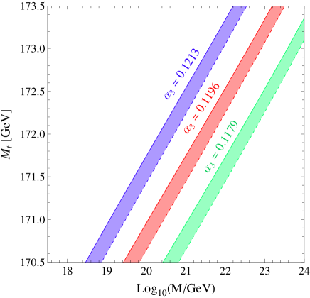
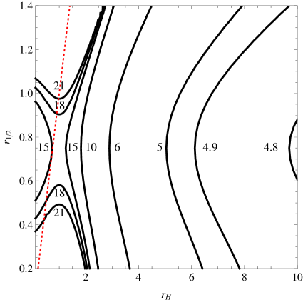
Figure 1: Left panel: Contour lines of $\mathcal{S}=0$ for different values of $\alpha_{3}(m_{Z})$ in the degenerate case of section VI.1. The solid (dashed) lines are obtained taking $m_{h}=126\,(125)$ GeV. Right panel: Contour lines of $\log_{10}M_{0}$ as a function of $r_{H}$ and $r_{1/2}$ leading to $\mathcal{S}=0$ in the non-degenerate case of section VI.2. We choose $m_{h}=125.1\,\rm{GeV}$, $m_{t}=172.5\,\rm{GeV}$, $\alpha_{3}(m_{Z})=0.1196$ and $\tan\beta=1$ for definiteness. Along the dotted straight line ($r_{1/2}=r_{H}$) the quadratic corrections can be understood as a generalization of the Veltman condition.

VI.2 A simple non-degenerate case

A simple non-degenerate case is the scenario where at the scale $\mathcal{Q}_{m}$ the sfermion, electroweakino and Higgs sectors have each one a respective common mass $M_{0}$, $M_{1/2}$ and $M_{H}$ as:

$$m_{Q}=m_{U}=m_{D}=m_{L}=m_{E}\equiv M_{0},\quad M_{1}=M_{2}=\mu\equiv M_{1/2},\quad m_{H}\equiv M_{H}\,\,.$$ (52)

In this case we can express $\Delta m^{2}(\mathcal{Q}_{m})$ as

$$\Delta m^{2}(\mathcal{Q}_{m})=\Delta_{f}m^{2}(\mathcal{Q}_{m})+\Delta_{\ell}m^{2}(\mathcal{Q}_{m})$$ (53)

with 

$$\Delta_{f}m^{2}(\mathcal{Q}_{m}) = \frac{1}{32\pi^{2}}\left\{(12y_{t}^{2}+12y_{b}^{2}+4y_{\tau}^{2})M_{0}^{2}-4GM_{1/2}^{2}-(6\lambda-G)M_{H}^{2}\right\}~{},$$ (54)

$$\Delta_{\ell}m^{2}(\mathcal{Q}_{m}) = \frac{1}{32\pi^{2}}\bigg{\{}-\left[(12y_{t}^{2}+12y_{b}^{2}+4y_{\tau}^{2})M_{0}^{2}+(6y_{t}^{2}X_{t}^{2}+6y_{b}^{2}X_{b}^{2}+2y_{\tau}^{2}X^{2}_{\tau})\right]\log\frac{M_{0}^{2}}{Q_{m}^{2}}$$ (55)

$$+ 4GM_{1/2}^{2}f_{\beta}\log\frac{M_{1/2}^{2}}{Q_{m}^{2}}+(6\lambda-G)M_{H}^{2}\log\frac{M_{H}^{2}}{Q_{m}^{2}}\bigg{\}}~{},$$

where $G=(g_{Y}^{2}+3g_{2}^{2})/2$, $f_{\beta}=2+\sin 2\beta$ and all parameters are understood at the scale $\mathcal{Q}_{m}$. For definiteness we take $\mathcal{Q}_{m}=M_{0}$ hereafter. It follows

$$\Delta_{f}m^{2}(\mathcal{Q}_{m}) = \frac{M_{0}^{2}}{32\pi^{2}v^{2}}\Big{\{}\sum_{f}n_{f}m_{f}^{2}\,-4(2m_{W}^{2}+m_{Z}^{2})r_{1/2}^{2}-(3m_{h}^{2}-2m_{W}^{2}-m_{Z}^{2})r_{H}^{2}\Big{\}}~{},~{}~{}~{}~{}~{}~{}~{}~{}~{}$$ (56)

$$\Delta_{\ell}m^{2}(\mathcal{Q}_{m}) = \frac{M_{0}^{2}}{32\pi^{2}v^{2}}\Big{\{}4f_{\beta}(2m_{W}^{2}+m_{Z}^{2})r_{1/2}^{2}\log r_{1/2}^{2}+(3m_{h}^{2}-2m_{W}^{2}-m_{Z}^{2})r_{H}^{2}\log r_{H}^{2}\Big{\}}~{},~{}$$

where $r_{H}=M_{H}/M_{0}$, $r_{1/2}=M_{1/2}/M_{0}$ and all masses are running.

For $r_{H}=r_{1/2}$ the right hand side of Eq. (56) coincides with the quadratic divergences that one derives from the SM effective potential by using as regulators the cutoff $\Lambda_{F}=M_{0}$ for fermions and the cutoff $\Lambda_{B}=M_{1/2}=M_{H}$ for bosons . In this case the requirement $\Delta_{f}m^{2}=0$ can be interpreted as a generalization of the Veltman condition expressing the Higgs quadratic divergence in terms of SM parameters and cutoffs . However also the logarithmic corrections are sizeable and contribute to destabilizing the potential. With the constraint $r_{H}=r_{1/2}$, $\Delta_{\ell}m^{2}$ is negligible only when $r_{H}=r_{1/2}\approx 1$. Correspondingly the condition $\Delta m^{2}=0$ with cutoffs at the TeV scale is not possible anymore.

However, for $r_{H}\neq r_{1/2}$ the stability under perturbative corrections can still be fulfilled at scales of $\mathcal{O}(100$ TeV) if one requires the cancellation of the total correction $\Delta m^{2}$. This can be seen in the right panel of Fig. 1 where the constraints on $r_{H}$ and $r_{1/2}$ leading to $\mathcal{S}=0$ (solid curves) are plotted for several values of $M_{0}$. The figure is obtained using Eqs. (56) and (LABEL:eq-ndDeltam2Loop) with $\tan\beta=5$, and running the SM parameter at NNLO with boundary conditions $m_{h}=125.1$ GeV, $M_{t}=172\,$GeV and $\alpha_{3}=0.1196$ at the electroweak scale as explained in Ref. Masina:2013wja . The former case, $r_{H}=r_{1/2}$, is exhibited as the dotted straight line in the right panel of Fig. 1 where we can see that stability can be achieved for sub-Planckian scales.

VI.3 General soft breaking terms

In principle one expects that all soft breaking parameters will be different at the scale $\mathcal{Q}_{m}$. In this general case the finite threshold contribution to the SM Higgs mass parameter is given by Eq. (46). The required condition for keeping $\Delta m^{2}$ at the order of the electroweak scale is then a hypersurface in the multidimensional space of supersymmetric parameters $(m_{Q},m_{U},m_{D},m_{L},m_{E},A_{t},A_{b},A_{\tau},m_{1},m_{2},\mu,M_{1},M_{2})$. In the next section some of these hypersurfaces are analyzed numerically for the case of negligible Fayet-Iliopoulos (FI) contribution .

Before closing this section a couple of comments are in order. In this section we have assumed $m^{2}(\mathcal{Q}_{m})$ at the electroweak scale without specifing the origin of such a value. The main ideas to naturally produce $m^{2}(\mathcal{Q}_{m})$ at the electroweak scale are twofold:

• If, i) the whole MSSM Higgs sector is at the electroweak scale (in which case the LE effective theory is not the SM but a two Higgs doublet model), and ii) the masses of the supersymmetric partners are in the low TeV region (i.e. $\mathcal{Q}_{m}\not\gg\mathcal{Q}_{EW}$), then $m^{2}(\mathcal{Q}_{m})$ is at the electroweak scale. Moreover the requirement $\left|\Delta m^{2}(\mathcal{Q}_{m})\right|\lesssim\mathcal{O}(100\,{\rm GeV})^{2}$ is also automatically satisfied. This parameter configuration might be excluded soon by the LHC lower bounds on heavy Higgs and superpartner masses and we will not further discuss it.

• For $\tan\beta\gg 1$ the squared mass $m^{2}(\mathcal{Q}_{m})$ is similar to $m_{2}^{2}(\mathcal{Q}_{m})$ [cf. Eq. (IV.2)]. The value of the latter is naturally small in the FP parameter region of the MSSM. This possibility has been broadly studied in the literature Feng:1999zg although the modifications due to $\Delta m^{2}$ have been overlooked.

In the next section we will analyze the effects that the one-loop corrections have on the FP solution.

VII Numerical results: focus point solutions

In this section we concentrate on the FP solution including the one-loop radiative correction $\Delta m^{2}$. We stress that till now we have expressed $m^{2}(\mathcal{Q}_{m})$ and $\Delta m^{2}(\mathcal{Q}_{m})$ as functions of supersymmetric parameters evaluated at the scale $\mathcal{Q}_{m}$. However, in view of a more fundamental supersymmetry-breaking description, $m^{2}$ and $\Delta m^{2}$ should be re-expressed in terms of the supersymmetric parameters evaluated at the messenger scale $\mathcal{M}$ at which supersymmetry breaking is transmitted to the observable sector. As, depending on the supersymmetry breaking model, some of the parameters can unify at the messenger scale, the number of independent parameters at the scale $\mathcal{M}$ can be smaller (than what would show up at the scale $\mathcal{Q}_{m}$). So, the required relation to keep $\Delta m^{2}$ and $m^{2}(\mathcal{Q}_{m})$ of the order of the electroweak scale is simpler, and might appear more natural. This scenario is considered in this section assuming, at the scale $\mathcal{M}$, as a simple example the case 

$$m_{Q}(\mathcal{M})=m_{U}(\mathcal{M})=M_{0},\quad m_{1}(\mathcal{M})=m_{2}(\mathcal{M})=M_{H},\quad M_{a}(\mathcal{M})=M_{1/2}~{}.$$ (58)

From Eqs. (39) and (40) we can write the matching conditions as

$$m^{2}_{LE}\simeq m^{2}(\mathcal{Q}_{m})+\Delta m^{2}(\mathcal{Q}_{m})=\frac{1}{\tan^{2}\beta-1}\widetilde{m}_{1}^{2}-\frac{\tan^{2}\beta}{\tan^{2}\beta-1}\widetilde{m}_{2}^{2}$$ (59)

where $\Delta m^{2}$ is given by Eq. (46), and the subleading radiative contribution $2m^{2}\Delta Z_{h}$ from the wave function renormalization is neglected. For $\tan\beta\gg 1$, $\mu=\mathcal{O}(100\,\rm{GeV})$ and small $\Delta m^{2}$, the requirement $m^{2}(\mathcal{Q}_{m})=\mathcal{O}(100\,{\rm GeV})^{2}$ implies $\left|m_{H_{2}}^{2}\right|=\mathcal{O}(100\,$GeV)², where $m_{H_{1,2}}^{2}$ are defined in Eq. (23). For heavy supersymmetric spectrum this size of $m_{H_{2}}^{2}$ can be generated in the neighborhood of the FP solution Delgado:2014vha ; Delgado:2013gza which is radiatively led to $m^{2}_{H_{2}}=0$. However in the FP parameter region there is no general reason why $\Delta m^{2}$ should be small. In fact the presence of $\Delta m^{2}$ can distort the standard FP solution usually considered in the literature. In this section we numerically analyze the parameter space of these modified FP solutions .

As it was mentioned in the previous section, it is useful to re-express the supersymmetric parameters of Eq. (59) in terms of their values at the high scale $\mathcal{M}$. On dimensional grounds we can rewrite them as

$$m_{X}^{2}(\mathcal{Q}_{m}) =m_{X}^{2}+\eta_{Q}^{X}[\mathcal{Q}_{m},\mathcal{M}](m_{Q}^{2}+m_{U}^{2}+m_{2}^{2})+\sum_{a,b}\eta_{ab}^{X}[\mathcal{Q}_{m},\mathcal{M}]M_{a}M_{b}$$

$$+\sum_{a}\eta_{aA}^{X}[\mathcal{Q}_{m},\mathcal{M}]M_{a}A_{0}+\eta_{A}^{X}[\mathcal{Q}_{m},\mathcal{M}]A_{0}^{2}~{},$$

$$A_{t}(\mathcal{Q}_{m}) =A_{0}+f_{A}[\mathcal{Q}_{m},\mathcal{M}]A_{0}+\sum_{a}f_{a}[\mathcal{Q}_{m},\mathcal{M}]M_{a}~{},$$ (60)

where $A_{0}$, $m^{2}_{X}$ and $M_{a}$ (with $X=H_{i},Q_{L},U_{R},D_{R}$ and $a=1,2,3$) are respectively the stop tri-linear mixing parameter, the sfermion masses and the Majorana gaugino masses at the scale $\mathcal{M}$.

Concerning the numerical procedure, we assume moderately large values of $\tan\beta$ (namely $\tan\beta\simeq 10$) which allows to approximate $X_{t}\simeq A_{t}$ and to safely neglect all Yukawa couplings except that of the top quark. Moreover we set $A_{t}$ at the mass scale $\widetilde{\mathcal{Q}}^{2}\equiv m_{Q}(\mathcal{Q}_{m})m_{U}(\mathcal{Q}_{m})$ in such a way that the SM RG evolution of the quartic coupling

$$\lambda(\widetilde{\mathcal{Q}})=\frac{1}{4}(g_{2}^{2}(\widetilde{\mathcal{Q}})+g_{Y}^{2}(\widetilde{\mathcal{Q}}))\cos^{2}2\beta+\frac{3}{8\pi}y_{t}^{4}(\widetilde{\mathcal{Q}})X_{t}^{2}\left(1-\frac{X_{t}^{2}}{12}\right)$$ (61)

from $\widetilde{\mathcal{Q}}$ to $\mathcal{Q}_{EW}$ reproduces the Higgs mass observation, namely $\lambda(\mathcal{Q}_{EW})\approx(m_{h}/v)^{2}/2$. For the functions $\eta^{X}[\mathcal{Q}_{m},\mathcal{M}]$ and $f[\mathcal{Q}_{m},\mathcal{M}]$, which were obtained semi-analytically for $\mathcal{Q}_{m}=2\,$TeV and $\mu\sim 100\,$GeV in Ref. Delgado:2014vha , we use some simple generalized formulas where the effect of possible heavy Higgsinos is incorporated . Finally, as fundamental description of the supersymmetric parameters, we consider the relations in Eq. (58).

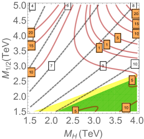
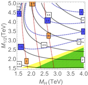
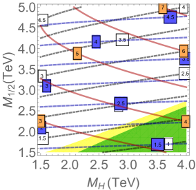
Figure 2: Left panel: Contour lines of $\log_{10}\mathcal{M}/GeV$ (white labels) and stability parameter $\mathcal{S}$ (orange labels) for $M_{0}=0$, and light Higgsinos, $\mu=100$ GeV. The (yellow) external shadowed region corresponds to $m_{U}(\mathcal{Q}_{m})<750$ GeV and the (green) internal shadowed region corresponds to $m_{U}^{2}(\mathcal{Q}_{m})<0$. Middle panel: Corresponding contour lines of constant $m_{Q}(\mathcal{Q}_{m})$ (solid black), $m_{U}(\mathcal{Q}_{m})$ (dashed blue) and $m_{H}(\mathcal{Q}_{m})$ (dash dotted red). Right panel: Corresponding contour lines of constant $M_{3}(\mathcal{Q}_{m})$ (solid red), $M_{2}(\mathcal{Q}_{m})$ (dashed blue) and $M_{1}(\mathcal{Q}_{m})$ (dash dotted black). Labels in the middle and right panels are in TeV units.

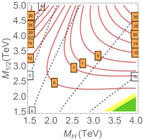
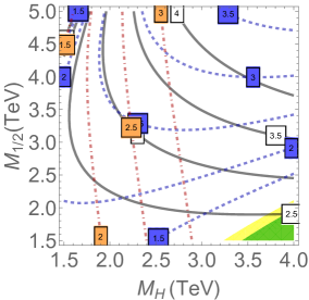
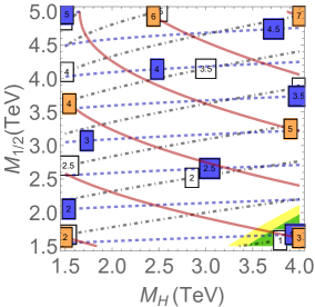
Figure 3: The same as in Fig. 2 but for $M_{0}=2$ TeV.

Figs. 2, 3, 4 and 5 display the values of fundamental parameters and their corresponding mass spectra leading to $m^{2}_{LE}\sim(100\,{\rm GeV})^{2}$. In the left panels of the figures we plot contour (black dashed) lines for constant values of $\log_{10}(\mathcal{M}/\textrm{GeV})$ such that Eq. (59) at tree level is fulfilled, and contour (solid red) lines for the stability parameter $\mathcal{S}$ of the one-loop radiative corrections (cf. Eqs. (46) and (48)). Similarly, the contour lines of $m_{Q}(\mathcal{Q}_{m})$ (solid black), $m_{U}(\mathcal{Q}_{m})$ (dashed blue) and $m_{H}(\mathcal{Q}_{m})$ (dash-dotted red) are shown in the middle panels, whereas the contour lines of $M_{3}(\mathcal{Q}_{m})$ (solid red), $M_{2}(\mathcal{Q}_{m})$ (dashed blue) and $M_{1}(\mathcal{Q}_{m})$ (dash-dotted black) are depicted in the right panels. We remind that the condition $m^{2}_{LE}\sim(100\,{\rm GeV})^{2}$ arises with no tuning between $m^{2}$ and $\Delta m^{2}$ when $\mathcal{S}=\mathcal{O}(1)$.

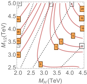
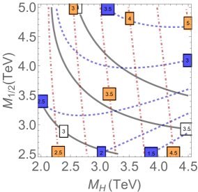
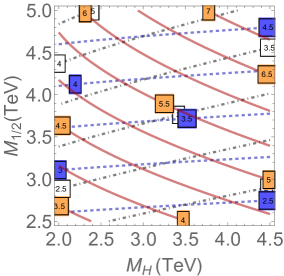
Figure 4: The same as in Fig. 3 but for $\mu=2$ TeV.

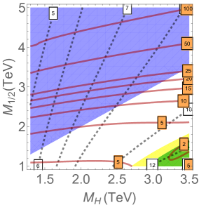
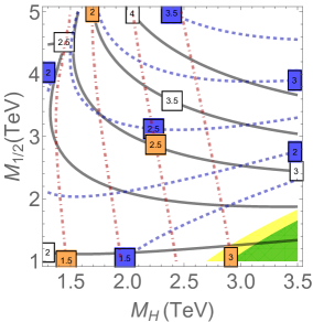
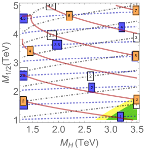
Figure 5: The same as in Fig. 3 but for $\mu=M_{1/2}$. In the (magenta) upper left shadowed region the soft breaking terms $m_{H_{U}}^{2}=m_{H_{D}}^{2}<0$ are tachyonic at the scale $\mathcal{M}$, although $m_{1}^{2}=m_{2}^{2}\equiv M_{H}^{2}>0$.

In Figs. 2 and 3 we consider the case $\mu\sim 100\,$GeV, and $M_{0}=0$, $M_{0}=2$ TeV, respectively, and in Figs. 4 and 5 the case with $M_{0}=2$ TeV and heavy and superheavy Higgsinos, with $\mu=2$ TeV and $\mu=M_{1/2}$, respectively. The region with $m_{U}(\mathcal{Q}_{m})<750$ GeV [$m_{U}^{2}(\mathcal{Q}_{m})<0$] corresponds to the yellow [green] shadowed area. In fact the yellow band corresponds to the FP for the light stop scenario Delgado:2014kqa .

As we can see from the general expression of radiative corrections, Eq. (46), gauge coupling terms should tend to compensate top Yukawa coupling terms when $M_{1/2},\,M_{H}>M_{0}$ . This is the case for the models analyzed in Figs. 2-4 where the stability condition is satisfied for $M_{1/2},\,M_{H}\gtrsim 3$ TeV. Finally this trend is broken for superheavy Higgsinos, as the $\mu=M_{1/2}$ case shown in Fig. 5. Here for very heavy gauginos, $M_{1/2}\gg 1$ TeV, the value of $M_{H}^{2}=m_{H_{u,d}}^{2}+\mu^{2}$ becomes very large and the condition $\mathcal{S}=1$ is overshot. Therefore the stability condition requires lighter gauginos than scalars as we can see in Fig. 5.

VIII Outlook and conclusions

In view of the growing experimental evidence against the existence of sub-TeV new physics, and having in mind the naturalness problem of electroweak interactions, it is interesting to study the matching of the SM with possible UV completions solving the grand hierarchy problem. In general we expect that the presence of heavy mass states, coupled to the Higgs sector in the UV theory, would contribute at the matching scale $\mathcal{Q}_{m}$ as finite threshold corrections to the SM Higgs mass term: these finite contributions trigger the hierarchy problem and destabilize the electroweak minimum. Determining these corrections is then of utmost importance to quantify the stability/naturalness problem and at least to find the parameter conditions that the underlying (final) theory at the unification, or Planck, scale should eventually provide to solve it.

In this paper we have pursued this task for the simplest perturbative UV completion of the SM solving the hierarchy problem: the MSSM. Although we have focused on this model, the qualitative features presented in this paper are expected to hold in any perturbative UV theory aiming to solve the grand hierarchy problem. The key ingredient of our analysis is the one-loop effective potential improved by the renormalization group equations, and the renormalization-scale invariance of such a potential. As a battleground we have considered the Landau gauge and dimensional regularization in the $\overline{MS}$ renormalization scheme (at this level of the calculation, and for scalar and fermion fields integrated out, equivalent to the $\overline{DR}$). With these choices we have obtained the one-loop matching between the SM and MSSM Higgs sectors at the multi-TeV matching scale $\mathcal{Q}_{m}$, where the large leading logarithms between the high (unification) scale $\mathcal{M}$ and $\mathcal{Q}_{m}$ have been resummed.

Motivated by hints from experimental data, the matching has been performed assuming a large mass hierarchy between SM and non-SM fields, which allows to work in the unbroken electroweak symmetry phase. After having integrated the heavy fields out, the final one-loop identification between the SM mass term, $m^{2}_{SM}$, and the MSSM mass terms, $m_{I}^{2}$ (with $I=1,2,3$), is given by Eq. (40) which can be written as

$$m_{SM}^{2}=\left[-m_{1}^{2}c^{2}_{\beta}-m_{2}^{2}s^{2}_{\beta}+2m_{3}^{2}s_{\beta}c_{\beta}\right](1+2\Delta Z_{h})+\Delta m^{2}~{},$$ (62)

where the radiative contributions $\Delta Z_{h}$ and $\Delta m^{2}$ are respectively coming from the matching between the wave functions and quadratic interactions of the SM and the MSSM lightest CP-even Higgs. The main features of the matching are as follows:

• We have integrated out only heavy states from the MSSM in the effective potential. We have not integrated out the heavy modes from the light (SM) states, as in the Wilsonian action, which would have created a cutoff in the low energy theory. In this way we can still integrate momenta in the low energy theory up to infinity and then keep on using dimensional regularization for them.

• Using the scale independence of the effective potential the matching scale $\mathcal{Q}_{m}$ is completely arbitrary in the considered one-loop approximation. If all heavy masses are of similar order of magnitude (as in the high-scale supersymmetry scenario considered here), $\mathcal{Q}_{m}$ can be arbitrarily fixed at some intermediate value around them to avoid large logarithms and the breaking of perturbation theory at higher-loop orders. If very different heavy scales are present (as e.g. in split supersymmetry ArkaniHamed:2004yi ) then different matching processes should be subsequently applied (cf. e.g. Ref. Carena:2008rt ).

• The size of the squared mass parameter of the lightest-Higgs in the high energy theory, $m^{2}=-m_{1}^{2}c^{2}_{\beta}-m_{2}^{2}s^{2}_{\beta}+2m_{3}^{2}s_{\beta}c_{\beta}$, is not physically meaningful as it is strongly scale dependent. Its dependence is mostly compensated by the one of $2\Delta Z_{h}$ and $\Delta m^{2}$, so that the final one-loop scale dependence of the right hand side of Eq. (62) is as weak as that of the SM mass parameter (in particular the dependence including large masses appears only at two loops). The natural scale of the SM electroweak sector should hence be deduced considering the sum of $m^{2}$ and $\Delta m^{2}$ (the $\Delta Z_{h}$ effect is in general subleading), possibly at the scale $\mathcal{Q}_{m}$ to avoid perturbative problems. In particular, once the magnitude of $m^{2}(\mathcal{Q}_{m})$ is enforced to be of the order of the electroweak scale, the stability of the electroweak breaking conditions is guaranteed by $\mathcal{S}\equiv|\Delta m^{2}(\mathcal{Q}_{m})/m^{2}_{LE}(\mathcal{Q}_{m})|\lesssim 1$.

We now present a short list of results obtained in the present paper:

• When the non-SM fields are heavy and degenerate, the expression for $\Delta m^{2}$ at the matching scale $\mathcal{Q}_{m}$ reproduces the result obtained by Veltman in the SM using dimensional regularization and extracting the “quadratic” divergence as the residue of the pole in $d=2$ dimensions. Veltman then interpreted this result as the coefficient of the cutoff $\Lambda^{2}$, while we can express it as the coefficient of the common supersymmetric mass squared. Our result is thus consistent with Veltman’s and puts solid grounds in the understanding of the SM as an effective theory below the MSSM. As it is well known, the vanishing of the Veltman coefficient can only be achieved at (super)Planckian scales.

• When the MSSM fields are heavy, and of the same order of magnitude but not fully degenerate, the stability of the electroweak minimum provides a generalization of Veltman’s result, which amounts to introducing different cutoffs for the different SM sectors, plus a modification that is negligible only for a strictly non-hierarchical heavy spectrum. In particular by assuming the masses of the heavy Higgses and/or gauginos to be larger than those of sfermions, one can easily achieve the vanishing of $\Delta m^{2}$ at sub-Planckian scales.

• We have analyzed several cases where the MSSM mass parameters are generated at high scale, and transmitted to the observable sector by means of some mediators between the hidden and observable sectors, and we have determined the parameter regions where $m^{2}(\mathcal{Q}_{m})\sim(100\,\rm{GeV})^{2}$. However also the requirement $\Delta m^{2}(\mathcal{Q}_{m})\lesssim\mathcal{O}(100\,\textrm{GeV})^{2}$ should be imposed in order to achieve satisfactory electroweak breaking conditions. The parameter regions where also this latter requirement is realized turn out to provide a sort of generalized focus point conditions which include threshold effects.

Let us finally make some considerations about the physical significance of the (stability) regions where both $m^{2}_{LE}(\mathcal{Q}_{EW})=\mathcal{O}(100\,\textrm{GeV})^{2}$ and $\mathcal{S}\lesssim 1$ conditions are satisfied:

• As we have already mentioned, these regions are obtained by integrating out the heavy fields at one-loop. The procedure is performed at a renormalization scale nearby the energy scale of the heavy masses. The result is thus not jeopardized by large logarithms and it has no relevant one-loop scale dependence.

• The stability regions do depend on the threshold contributions we obtain from the effective potential in a particular (Landau) gauge. Therefore, in general, we could expect a gauge dependence in our results. However as we have performed the matching in the unbroken electroweak symmetry phase and upon integrating out only scalars and fermions (neither gauge nor Goldstone bosons), it turns out that our computation of the thresholds is gauge independent within the considered approximations.

• The effective potential depends on the particular renormalization scheme, and we have worked it out in the $\overline{MS}$ scheme which amounts to subtracting (to define the counter-term) the infinite term proportional to $\frac{2}{\epsilon}-\gamma_{E}+\log(4\pi)-\delta$ with $\delta=0$. In the $\overline{MS}$ scheme the finite term in the effective potential contributions coming from heavy fermions and scalars is proportional to the constant $\mathcal{C}=3/2$ [cf. Eq. (5)]. Subtracting a different infinite counter term (with $\delta\neq 0$, as e.g. in the $MS$ renormalization scheme or a variant thereof) would then lead to a shift in the constant $C$ as $C\to C+\delta$. Consequently for the degenerate and almost degenerate cases, the stability condition $\mathcal{S}=0$ leading respectively to the exact and generalized Veltman conditions (cf. sections VI.1 and VI.2 with $r_{1/2}\simeq r_{H}\simeq 1$) would receive additional contributions. Therefore, the Veltman-like conditions we obtain from the MSSM arise only in the $\overline{DR}$ scheme and are relevant for the matching with the SM effective theory in the $\overline{MS}$ renormalization scheme.

To conclude, given a scheme of supersymmetry breaking involving soft terms above the TeV scale, the threshold corrections to the Higgs mass parameters play a determinant role in the stability of the electroweak breaking conditions and the masses of the Higgs fields. In the present paper we have determined these threshold corrections in some MSSM scenarios with no relevant hierarchy in the heavy mass spectrum, and looked for soft-parameter relations that could alleviate the little hierarchy problem. Of course it is clear that a similar analysis can also be performed for any perturbative theory that UV completes the SM. Moreover an equivalent analysis can be done even if the low energy theory is itself some extension of the SM, as one in which there is an aligned extended Higgs sector Gunion:2002zf giving rise to e.g. a two Higgs doublet model. If the UV completion of the SM is not perturbative, as in the case of a composite Higgs, the calculation cannot rely on perturbation theory and different methods to evaluate threshold effects should be used Tavares:2013dga . In general, whatever the final UV completion of the SM is, we expect it could provide an answer to the question on why our electroweak vacuum is stable and insensitive to high scale physics.

Appendix A Radiative corrections to mass parameters

In this appendix we will present a detailed calculation of the radiative contributions to the mass parameters $\Delta m_{1}^{2}$, $\Delta m_{2}^{2}$ and $\Delta m_{3}^{2}$ in the MSSM arising from the different sectors of sfermions, charginos, neutralinos and the Higgs scalar sector.

A.1 Squarks and sleptons

The mass squared matrices for top and bottom squarks and for tau-sneutrinos and staus can be written as

$$M^{2}_{\tilde{t}}=\left(\begin{matrix}m_{Q}^{2}+Y_{t}^{2}h_{2}^{2}+\Pi_{\tilde{u}_{L}}&Y_{t}(A_{t}h_{2}-\mu h_{1})\\ Y_{t}(A_{t}h_{2}-\mu h_{1})&m_{U}^{2}+Y_{t}^{2}h_{2}^{2}+\Pi_{\tilde{u}_{R}}\end{matrix}\right)$$ (63)

$$M^{2}_{\tilde{b}}=\left(\begin{matrix}m_{Q}^{2}+Y_{b}^{2}h_{1}^{2}+\Pi_{\tilde{d}_{L}}&Y_{b}(A_{b}h_{1}-\mu h_{2})\\ Y_{b}(A_{b}h_{1}-\mu h_{2})&m_{D}^{2}+Y_{b}^{2}h_{1}^{2}+\Pi_{\tilde{d}_{R}}\end{matrix}\right)$$ (64)

$$M^{2}_{\tilde{\nu}_{\tau}}=\left(\begin{matrix}m_{L}^{2}+\Pi_{\tilde{\nu}_{L}}&0\\ 0&m_{N}^{2}\end{matrix}\right)$$ (65)

$$M^{2}_{\tilde{\tau}}=\left(\begin{matrix}m_{L}^{2}+Y_{\tau}^{2}h_{1}^{2}+\Pi_{\tilde{e}_{L}}&Y_{\tau}(A_{\tau}h_{1}-\mu h_{2})\\ Y_{\tau}(A_{\tau}h_{1}-\mu h_{2})&m_{E}^{2}+Y_{\tau}^{2}h_{1}^{2}+\Pi_{\tilde{e}_{R}}\end{matrix}\right)$$ (66)

where

$$\Pi_{\tilde{f}}=\frac{1}{2}\left[T_{3_{\tilde{f}}}\left(g_{Y}^{2}+g_{2}^{2}\right)-Q_{\tilde{f}}g_{Y}^{2}\right](h_{1}^{2}-h_{2}^{2})\,\,.$$ (67)

Using the expressions in Eq. (44) it is straightforward to find the corresponding contributions to $\Delta m^{2}_{1,2,3}$ as

$$\Delta m_{1}^{2} = \frac{2}{32\pi^{2}}\left\{3Y_{b}^{2}[G(m_{Q}^{2})+G(m_{D}^{2})]+Y_{\tau}^{2}[G(m_{L}^{2})+G(m_{E}^{2})]+\frac{3Y_{t}^{2}\mu^{2}}{m_{Q}^{2}-m_{U}^{2}}[G(m_{Q}^{2})-G(m_{U}^{2})]\right.$$

$$+ \frac{3Y_{b}^{2}A_{b}^{2}}{m_{Q}^{2}-m_{D}^{2}}[G(m_{Q}^{2})-G(m_{D}^{2})]+\frac{Y_{\tau}^{2}A_{\tau}^{2}}{m_{L}^{2}-m_{E}^{2}}[G(m_{L}^{2})-G(m_{E}^{2})]$$

$$- \left.\frac{g_{Y}^{2}}{2}[G(m_{Q}^{2})-2G(m_{U}^{2})+G(m_{D}^{2})-G(m_{L}^{2})+G(m_{E}^{2})]\right\}~{},$$

$$\Delta m_{2}^{2} = \frac{2}{32\pi^{2}}\left\{3Y_{t}^{2}[G(m_{Q}^{2})+G(m_{U}^{2})]+\frac{3Y_{t}^{2}A_{t}^{2}}{m_{Q}^{2}-m_{U}^{2}}[G(m_{Q}^{2})-G(m_{U}^{2})]\right.$$

$$+ \frac{3Y_{b}^{2}\mu^{2}}{m_{Q}^{2}-m_{D}^{2}}[G(m_{Q}^{2})-G(m_{D}^{2})]+\frac{Y_{\tau}^{2}\mu^{2}}{m_{L}^{2}-m_{E}^{2}}[G(m_{L}^{2})-G(m_{E}^{2})]$$

$$+ \left.\frac{g_{Y}^{2}}{2}[G(m_{Q}^{2})-2G(m_{U}^{2})+G(m_{D}^{2})-G(m_{L}^{2})+G(m_{E}^{2})]\right\}~{},$$

$$\Delta m_{3}^{2} = \frac{2}{32\pi^{2}}\left\{\frac{3Y_{t}^{2}\mu A_{t}}{m_{Q}^{2}-m_{U}^{2}}[G(m_{Q}^{2})-G(m_{U}^{2})]+\frac{3Y_{b}^{2}\mu A_{b}}{m_{Q}^{2}-m_{D}^{2}}[G(m_{Q}^{2})-G(m_{D}^{2})]\right.$$

$$+ \left.\frac{Y_{\tau}^{2}\mu A_{\tau}}{m_{L}^{2}-m_{E}^{2}}[G(m_{L}^{2})-G(m_{E}^{2})]\right\}\,\,,$$

with

$$G(m_{X}^{2})\equiv m_{X}^{2}\left[\log\frac{m_{X}^{2}}{\mathcal{Q}_{m}^{2}}-1-\delta\right]~{}.$$ (68)

Here the function $G$ has been generalized to the subtraction schemes having $\mathcal{C}=3/2+\delta$ in the scalar contributions of Eq. (5). Eq. (68) recovers Eq. (45) for the $\overline{MS}$ (or $\overline{DR}$) subtraction scheme where $\delta=0$.

If some of the masses are degenerate the following limit turns useful:

$$\lim_{y\to x}\frac{G(x^{2})-G(y^{2})}{x^{2}-y^{2}}=\log\frac{x^{2}}{\mathcal{Q}_{m}^{2}}-\delta\ .$$ (69)

A.2 Charginos

The squared mass matrix for the charginos can be written as

$$M^{2}_{ch}=\left(\begin{matrix}M_{2}^{2}+g_{2}^{2}h_{2}^{2}&g_{2}(M_{2}h_{1}+\mu h_{2})\\ g_{2}(M_{2}h_{1}+\mu^{*}h_{2})&\mu^{2}+g_{2}^{2}h_{1}^{2}\end{matrix}\right)\,\,.$$ (70)

We can then compute the corresponding contributions to $\Delta m_{1,2,3}^{2}$ as

$$\Delta m_{1}^{2}=\Delta m_{2}^{2}=-\frac{4}{32\pi^{2}}\frac{g_{2}^{2}}{M_{2}^{2}-\mu^{2}}\,[M_{2}^{2}G(M_{2}^{2})-\mu^{2}G(\mu^{2})]~{},$$ (71)

$$\Delta m_{3}^{2}=\frac{4}{32\pi^{2}}\frac{g_{2}^{2}\mu M_{2}}{M_{2}^{2}-\mu^{2}}\,[G(M_{2}^{2})-G(\mu^{2})]~{},$$ (72)

with $G$ defined in Eq. (68). In case of degenerate spectra the following limit is useful:

$$\lim_{y\to x}\frac{x^{2}G(x^{2})-y^{2}G(y^{2})}{x^{2}-y^{2}}=x^{2}\left(-1-2\delta+2\log\frac{x^{2}}{\mathcal{Q}_{m}^{2}}\right)$$ (73)

with $\delta=0$ in the $\overline{MS}$ or $\overline{DR}$ schemes.

A.3 Neutralinos

The squared mass matrix for the neutralinos can be written as

$$M^{2}_{ne}=\left(\begin{matrix}M_{1}^{2}+\frac{g_{Y}^{2}}{2}(h_{1}^{2}+h_{2}^{2})&-\frac{1}{2}g_{Y}g_{2}(h_{1}^{2}+h_{2}^{2})&-\frac{g_{Y}}{\sqrt{2}}(M_{1}h_{1}+\mu h_{2})&\frac{g_{Y}}{\sqrt{2}}(M_{1}h_{2}+\mu h_{1})\\ -\frac{1}{2}g_{Y}g_{2}(h_{1}^{2}+h_{2}^{2})&M_{2}^{2}+\frac{g_{2}^{2}}{2}(h_{1}^{2}+h_{2}^{2})&\frac{g_{2}}{\sqrt{2}}(M_{2}h_{1}+\mu h_{2})&-\frac{g_{2}}{\sqrt{2}}(M_{2}h_{2}+\mu h_{1})\\ -\frac{g_{1}}{\sqrt{2}}(M_{1}h_{1}+\mu h_{2})&\frac{g_{2}}{\sqrt{2}}(M_{2}h_{1}+\mu h_{2})&\mu^{2}+\frac{h_{1}^{2}}{2}(g_{Y}^{2}+g_{2}^{2})&-\frac{1}{2}h_{1}h_{2}(g_{Y}^{2}+g_{2}^{2})\\ \frac{g_{Y}}{\sqrt{2}}(M_{1}h_{2}+\mu h_{1})&-\frac{g_{2}}{\sqrt{2}}(M_{2}h_{2}+\mu h_{1})&-\frac{1}{2}h_{1}h_{2}(g_{Y}^{2}+g_{2}^{2})&\mu^{2}+\frac{h_{2}^{2}}{2}(g_{Y}^{2}+g_{2}^{2})\end{matrix}\right)\,\,.$$ (74)

The derivatives of the mass eigenvalues with respect to the backgrounds $\phi_{j}\equiv(h_{1}^{2},h_{2}^{2},h_{1}h_{2})$ can be easily computed following the techniques introduced in Ref. Ibrahim:2002zk . The squared mass eigenvalues are given by the solutions of the equation defined by the characteristic polynomial

$$\det(M^{\dagger}M-\lambda)\equiv\sum_{n}c^{(n)}(\phi_{j})\lambda^{n}=0$$ (75)

where the coefficients of the characteristic polynomial are functions of $h_{1}^{2}$, $h_{2}^{2}$ and $h_{1}h_{2}$. Differentiating (75) with respect to $\phi_{j}$ we obtain the required expressions

$$\left.\frac{\partial\lambda}{\partial\phi_{j}}\right|_{h_{i}=0}=-\left.\frac{\sum_{n}\frac{\partial c^{(n)}(\phi_{j})}{\partial\phi_{j}}\lambda^{n}}{\sum_{n}nc^{(n)}(\phi_{j})\lambda^{n-1}}\right|_{h_{i}=0}$$ (76)

where on the right hand side $\lambda$ denotes the squared mass eigenvalues.

The calculation of $\Delta m_{1,2,3}^{2}$ is now straightforward and gives

$$\Delta m_{1}^{2} =\Delta m_{2}^{2}=-\frac{2}{32\pi^{2}}\left\{\frac{g_{Y}^{2}}{M_{1}^{2}-\mu^{2}}[M_{1}^{2}G(M_{1}^{2})-\mu^{2}G(\mu^{2})]\right.$$

$$+\left.\frac{g_{2}^{2}}{M_{2}^{2}-\mu^{2}}[M_{2}^{2}G(M_{2}^{2})-\mu^{2}G(\mu^{2})]\right\}$$

$$\Delta m_{3}^{2} =\frac{2}{32\pi^{2}}\left\{\frac{g_{Y}^{2}M_{1}\mu}{M_{1}^{2}-\mu^{2}}[G(M_{1}^{2})-G(\mu^{2})]+\frac{g_{2}^{2}M_{2}\mu}{M_{2}^{2}-\mu^{2}}[G(M_{2}^{2})-G(\mu^{2})]\right\}\,\,.$$ (77)

In the case of equal masses we can use the limiting behavior in Eqs. (69) and (73).

A.4 Higgs scalar sector

The general tree level potential for the scalar sector is given by

$$V =m_{1}^{2}|H_{1}|^{2}+m_{2}^{2}|H_{2}|^{2}+m_{3}^{2}(H_{1}\cdot H_{2}+h.c.)+\frac{g_{Z}^{2}}{2}(|H_{2}|^{2}-|H_{1}|^{2})^{2}$$

$$+\frac{g_{2}^{2}}{2}|H_{2}^{+}H_{1}^{0*}+H_{1}^{-*}H_{2}^{0}|^{2}$$ (78)

where $H_{1}\cdot H_{2}=H_{1}^{a}\varepsilon_{ab}H_{2}^{b}$ with $\varepsilon_{12}=-1$. The squared mass matrices for scalars [in the basis $(\textrm{Re}\,H_{1}^{0},\textrm{Re}\,H_{2}^{0})$], pseudoscalars [in the basis $(\textrm{Im}\,H_{1}^{0},\textrm{Im}\,H_{2}^{0})$] and charged scalars [in the basis $(H_{2}^{+},H_{1}^{-*})$] are

$$M^{2}_{S}=\left(\begin{matrix}m_{1}^{2}-g_{Z}^{2}(h_{2}^{2}-3h_{1}^{2})&-m_{3}^{2}-2g_{Z}^{2}h_{1}h_{2}\\ -m_{3}^{2}-2g_{Z}^{2}h_{1}h_{2}&m_{2}^{2}+g_{Z}^{2}(3h_{2}^{2}-h_{1}^{2})\end{matrix}\right)$$ (79)

$$M^{2}_{P}=\left(\begin{matrix}m_{1}^{2}-g_{Z}^{2}(h_{2}^{2}-h_{1}^{2})&m_{3}^{2}\\ m_{3}^{2}&m_{2}^{2}+g_{Z}^{2}(h_{2}^{2}-h_{1}^{2})\end{matrix}\right)$$ (80)

$$M^{2}_{C}=\left(\begin{matrix}m_{2}^{2}+g_{Z}^{2}(h_{2}^{2}-h_{1}^{2})+\frac{g_{2}^{2}}{2}h_{1}^{2}&m_{3}^{2}+\frac{g_{2}^{2}}{2}h_{1}h_{2}\\ m_{3}^{2}+\frac{g_{2}^{2}}{2}h_{1}h_{2}&m_{1}^{2}-g_{Z}^{2}(h_{2}^{2}-h_{1}^{2})+\frac{g_{2}^{2}}{2}h_{2}^{2}\end{matrix}\right)\,\,.$$ (81)

For each of the previous matrices there are two eigenstates in the unbroken phase ($h_{i}=0$), $H_{SM}=c_{\beta}H_{1}+s_{\beta}\tilde{H}_{2}^{*}$ with mass eigenvalue $-m^{2}$, and $H_{h}=-s_{\beta}H_{1}+c_{\beta}\tilde{H}_{2}^{*}$ with mass eigenvalue $m_{H}^{2}=m_{1}^{2}+m_{2}^{2}+m^{2}$. The doublet $H_{SM}$ is identified with the SM Higgs doublet, and we then exclude its contribution to $\Delta m^{2}$. Using Eq. (76) one obtains that the heavy Higgs contributions are given by

$$\Delta m_{1}^{2} =\frac{1}{32\pi^{2}}\,\frac{G(m_{H}^{2})}{m_{1}^{2}+m_{2}^{2}+2m^{2}}\left[2g_{Z}^{2}(3m_{1}^{2}-2m_{2}^{2}+m^{2})+g_{2}^{2}(m_{2}^{2}+m^{2})\right]$$

$$\Delta m_{2}^{2} =\frac{1}{32\pi^{2}}\,\frac{G(m_{H}^{2})}{m_{1}^{2}+m_{2}^{2}+2m^{2}}\left[2g_{Z}^{2}(3m_{2}^{2}-2m_{1}^{2}+m^{2})+g_{2}^{2}(m_{1}^{2}+m^{2})\right]$$

$$\Delta m_{3}^{2} =\frac{1}{32\pi^{2}}\,\frac{G(m_{H}^{2})}{m_{1}^{2}+m_{2}^{2}+2m^{2}}\left[-2g_{Z}^{2}-g_{2}^{2}\right]m_{3}^{2}~{}.$$ (82)

Using now the matching conditions (31), Eqs. (82) can be also written as

$$\Delta m_{1}^{2} =\frac{1}{32\pi^{2}}\,G(m_{H}^{2})\left[-4g_{Z}^{2}\cos 2\beta+2g_{Z}^{2}\sin^{2}\beta+g_{2}^{2}\cos^{2}\beta\right]$$

$$\Delta m_{2}^{2} =\frac{1}{32\pi^{2}}\,G(m_{H}^{2})\left[4g_{Z}^{2}\cos 2\beta+2g_{Z}^{2}\cos^{2}\beta+g_{2}^{2}\sin^{2}\beta\right]$$

$$\Delta m_{3}^{2} =\frac{1}{32\pi^{2}}\,G(m_{H}^{2})\left[-2g_{Z}^{2}-g_{2}^{2}\right]\sin\beta\cos\beta\,\,.$$ (83)

Appendix B One-loop scale invariance of the matching

In section III we showed that by construction the one-loop matching conditions obtained via one-loop RG-improved effective potentials are independent of the choice of $\mathcal{Q}_{m}$. Here we use this property to check our finding (46).

The matching condition (40) led to (cf. section III.2)

$$m^{2}_{LE}(\mathcal{Q}_{m})=m^{2}(\mathcal{Q}_{m})[1+2\Delta Z_{h}(\mathcal{Q}_{m})]+\Delta m^{2}\ ,$$ (84)

where [cf. Eqs. (38) and (39)]

$$m^{2} = -m_{1}^{2}\cos^{2}\beta-m_{2}^{2}\sin^{2}\beta+m_{3}^{2}\sin 2\beta~{},$$ (85)

$$\Delta m^{2} = -\Delta m_{1}^{2}\cos^{2}\beta-\Delta m_{2}^{2}\sin^{2}\beta+\Delta m_{3}^{2}\sin 2\beta~{},$$ (86)

$$\tan 2\beta = 2\widetilde{m}_{3}^{2}/(\widetilde{m}_{2}^{2}-\widetilde{m}_{1}^{2})~{}.$$ (87)

The one-loop scale invariance imposes that in Eq. (84) the one-loop $\mathcal{Q}_{m}$ dependence of the right hand side is the same of the SM. Here we check this issue.

The total derivative of the right hand side (RHS) in Eq. (84) with respect to $\log\mathcal{Q}_{m}$ is given by 

$$\beta_{RHS}=-\beta_{\widetilde{m}_{1}^{2}}\cos^{2}\beta-\beta_{\widetilde{m}_{2}^{2}}\sin^{2}\beta+\beta_{\widetilde{m}_{3}^{2}}\sin 2\beta+m^{2}(1+2\gamma_{h}-2\gamma_{h_{LE}})~{},$$ (88)

with

$$\widetilde{m}_{I}^{2}=m_{I}^{2}+\Delta m_{I}^{2}=m_{I}^{2}+\sum_{r}\Delta m_{I,r}^{2}~{},\qquad\beta_{\widetilde{m}_{I}^{2}}=\beta_{m_{I}^{2}}+\beta_{\Delta m_{I}^{2}}\equiv\beta_{m_{I}^{2}}-\sum_{r}\Delta_{I}^{r}~{},$$ (89)

where the index $r$ runs over the heavy fields as in Eq. (42). The (one-loop) contribution $\Delta m_{I}^{r}$ can hence be deduced from the one-loop $\mathcal{Q}$ dependence of $\Delta m^{2}_{I,r}$. Each quantity $\Delta m^{2}_{I,r}$ is provided in appendix A and can be decomposed into its logarithmic and non-logarithmic contributions as follows:

$$\Delta m_{I,r}^{2}=\Delta^{r}_{\ell}m_{I}^{2}+\Delta_{f}^{r}m_{I}^{2}\equiv\frac{1}{32\pi^{2}}\ell_{I,r}+\frac{1}{32\pi^{2}}f_{I,r}\,.$$ (90)

In particular $\ell_{I,r}=32\pi^{2}\Delta m_{I,r}^{2}(G\to\widetilde{G})$, with $\widetilde{G}(x^{2})\equiv x^{2}\log(x^{2}/\mathcal{Q}^{2})$, represents all terms proportional to logarithms of squared masses over $\mathcal{Q}_{m}^{2}$, and $f_{I,r}=32\pi^{2}\Delta m_{I,r}^{2}(G\to\overline{G})$ with $\overline{G}(x^{2})\equiv-x^{2}(1+\delta)$ contains all non-logarithmic terms ($\delta=0$ in the $\overline{MS}$ and $\overline{DR}$). At one loop each $f_{I,r}$ is thus independent of $\mathcal{Q}_{m}$, and it results $\Delta_{I}^{r}=\partial\Delta m_{I,r}^{2}/\partial\mathcal{Q}$.

The values of $\sum_{r}\Delta_{I}^{r}$ are determined in steps considering the contributions computed in appendix A for each sector. It comes out from sfermions

$$(16\pi^{2})\Delta_{1}^{\widetilde{f}} =6Y_{b}^{2}(m_{Q}^{2}+m_{D}^{2}+A_{b}^{2})+2Y_{\tau}^{2}(m_{L}^{2}+m_{E}^{2}+A_{\tau}^{2})+6Y_{t}^{2}\mu^{2}$$

$$-\frac{3}{5}g_{1}^{2}(m_{Q}^{2}-2m_{U}^{2}+m_{D}^{2}-m_{L}^{2}+m_{E}^{2})~{},$$

$$(16\pi^{2})\Delta_{2}^{\widetilde{f}} =6Y_{t}^{2}(m_{Q}^{2}+m_{U}^{2}+A_{t}^{2})+6Y_{b}^{2}\mu^{2}+2h_{\tau}^{2}\mu^{2}$$

$$+\frac{3}{5}g_{1}^{2}(m_{Q}^{2}-2m_{U}^{2}+m_{D}^{2}-m_{L}^{2}+m_{E}^{2})~{},$$

$$(16\pi^{2})\Delta_{3}^{\widetilde{f}} =6Y_{t}^{2}\mu A_{t}+6Y_{b}^{2}\mu A_{b}+2Y_{\tau}^{2}\mu A_{\tau}~{},$$ (91)

from charginos

$$(16\pi^{2})\Delta_{1}^{\widetilde{\chi}^{\pm}} =\Delta_{2}^{\widetilde{\chi}^{\pm}}=-4g_{2}^{2}(M_{2}^{2}+\mu^{2})~{},$$

$$(16\pi^{2})\Delta_{3}^{\widetilde{\chi}^{\pm}} =4g_{2}^{2}\mu M_{2}~{},$$ (92)

from neutralinos

$$(16\pi^{2})\Delta_{1}^{\widetilde{\chi}^{0}} =\Delta_{2}^{\widetilde{\chi}^{0}}=-2g_{2}^{2}(M_{2}^{2}+\mu^{2})-\frac{6}{5}g_{1}^{2}(M_{1}^{2}+\mu^{2})~{},$$

$$(16\pi^{2})\Delta_{3}^{\widetilde{\chi}^{0}} =2g_{2}^{2}M_{2}\mu+\frac{6}{5}g_{1}^{2}M_{1}\mu~{},$$ (93)

and from the scalar, pseudoscalar and charged Higgs sector

$$(16\pi^{2})\Delta_{1}^{H} =\frac{m_{1}^{2}+m_{2}^{2}+m^{2}}{m_{1}^{2}+m_{2}^{2}+2m^{2}}\left[2g_{Z}^{2}(3m_{1}^{2}-2m_{2}^{2}+m^{2})+g_{2}^{2}(m_{2}^{2}+m^{2})\right]~{},$$

$$(16\pi^{2})\Delta_{2}^{H} =\frac{m_{1}^{2}+m_{2}^{2}+m^{2}}{m_{1}^{2}+m_{2}^{2}+2m^{2}}\left[2g_{Z}^{2}(3m_{2}^{2}-2m_{1}^{2}+m^{2})+g_{2}^{2}(m_{1}^{2}+m^{2})\right]~{},$$

$$(16\pi^{2})\Delta_{3}^{H} =-\frac{m_{1}^{2}+m_{2}^{2}+m^{2}}{m_{1}^{2}+m_{2}^{2}+2m^{2}}\left[2g_{Z}^{2}+g_{2}^{2}\right]m_{3}^{2}~{}.$$ (94)

Now using Eq. (89) and the MSSM one-loop $\beta$-functions Castano:1993ri

$$(16\pi^{2})\beta_{m_{1}^{2}} =6Y_{b}^{2}(m_{Q}^{2}+m_{D}^{2}+m_{1}^{2}+A_{b}^{2})+2Y_{\tau}^{2}(m_{L}^{2}+m_{E}^{2}+m_{1}^{2}+A_{\tau}^{2})$$

$$+(6Y_{t}^{2}-6g_{2}^{2}-\frac{6}{5}g_{1}^{2})\mu^{2}-6g_{2}^{2}M_{2}^{2}-\frac{6}{5}g_{1}^{2}M_{1}^{2}-\frac{3}{5}g_{1}^{2}S~{},$$

$$(16\pi^{2})\beta_{m_{2}^{2}} =6Y_{t}^{2}(m_{Q}^{2}+m_{U}^{2}+m_{2}^{2}+A_{t}^{2})$$

$$+(6Y_{b}^{2}+2Y_{\tau}^{2}-6g_{2}^{2}-\frac{6}{5}g_{1}^{2})\mu^{2}-6g_{2}^{2}M_{2}^{2}-\frac{6}{5}g_{1}^{2}M_{1}^{2}+\frac{3}{5}g_{1}^{2}S~{},$$

$$(16\pi^{2})\beta_{m_{3}^{2}} =(3Y_{t}^{2}+3Y_{b}^{2}+Y_{\tau}^{2}-3g_{2}^{2}-\frac{3}{5}g_{1}^{2})m_{3}^{2}$$

$$+(6Y_{t}^{2}A_{t}^{2}+6Y_{b}^{2}A_{b}+2Y_{\tau}^{2}A_{\tau}+6g_{2}^{2}M_{2}+\frac{6}{5}g_{1}^{2}M_{1})\mu~{},$$ (95)

where $S=m_{Q}^{2}-2m_{U}^{2}+m_{D}^{2}-m_{L}^{2}+m_{E}^{2}+m_{2}^{2}-m_{1}^{2}$, we can write

$$(16\pi^{2})\beta_{\widetilde{m}_{1}^{2}} =(6Y_{b}^{2}+2Y_{\tau}^{2}-2g_{Z}^{2}-g_{2}^{2})m_{1}^{2}-m^{2}[(2g_{Z}^{2}+g_{2}^{2})\sin^{2}\beta+6g_{Z}^{2}\cos 2\beta]$$

$$(16\pi^{2})\beta_{\widetilde{m}_{2}^{2}} =(6Y_{t}^{2}-2g_{Z}^{2}-g_{2}^{2})m_{2}^{2}-m^{2}[(2g_{Z}^{2}+g_{2}^{2})\cos^{2}\beta-6g_{Z}^{2}\cos 2\beta]$$

$$(16\pi^{2})\beta_{\widetilde{m}_{3}^{2}} =(3Y_{t}^{2}+3Y_{b}^{2}+Y_{\tau}^{2}-2g_{Z}^{2}-g_{2}^{2})m_{3}^{2}-m^{2}(2g_{Z}^{2}+g_{2}^{2})\sin\beta\cos\beta\ .$$ (96)

Plugging these expressions in Eq. (88) yields

$$\beta_{RHS} =6Y_{t}^{2}(\sin\beta\cos\beta\,m_{3}^{2}-\sin^{2}\beta\,m_{2}^{2})+(6Y_{b}^{2}+2Y_{\tau}^{2})(\sin\beta\cos\beta\,m_{3}^{2}-\cos^{2}\beta\,m_{1}^{2})$$

$$-(2g_{Z}^{2}+g_{2}^{2})(-\cos^{2}\beta m_{1}^{2}-\sin^{2}\beta m_{2}^{2}+\sin 2\beta m_{3}^{2})+(6g_{Z}^{2}c_{2\beta}^{2}+2\Delta\gamma)m^{2}\ ,$$ (97)

where $\Delta\gamma=\gamma_{h}-\gamma_{LE}=\gamma_{1}\cos^{2}\beta+\gamma_{2}\sin^{2}\beta-\gamma_{h_{LE}}=-\frac{3}{2}(\frac{1}{5}g_{1}^{2}+g_{2}^{2})$. (This difference between $\gamma_{h}$ and $\gamma_{LE}$ is caused by the heavy electroweakinos.) Finally one imposes the tree-level matching conditions of Eqs. (31) and (33), and obtains

$$\beta_{RHS}=\left(6y_{t}^{2}+6y_{b}^{2}+2y_{\tau}^{2}+6\lambda-\frac{9}{10}g_{1}^{2}-\frac{9}{2}g_{2}^{2}\right)m^{2}~{}.$$ (98)

Eq. (98) thus agrees with the $\beta$ function of the quadratic term in the SM Luo:2002ey . Note that in Eq. (98) the use of tree-level relations within the one-loop $\beta$ functions is justified by the fact that we are working at one-loop order.

Before concluding, notice that the splitting (90) turns out to be useful also for $\Delta m^{2}$. In such a case it reads as

$$\Delta m^{2} =\Delta_{\ell}m^{2}+\Delta_{f}m^{2}~{},$$

$$-\Delta_{\ell}m^{2} =\Delta_{\ell}m_{1}^{2}\cos^{2}\beta+\Delta_{\ell}m^{2}_{2}\sin^{2}\beta-\Delta_{\ell}m^{2}_{3}\sin 2\beta~{},$$

$$-\Delta_{f}m^{2} =\Delta_{f}m^{2}_{1}\cos^{2}\beta+\Delta_{f}m^{2}_{2}\sin^{2}\beta-\Delta_{f}m^{2}_{3}\sin 2\beta~{}$$ (99)

although, as we already noticed, the splitting into a logarithmic (or one-loop scale dependent) and non-logarithmic (or one-loop scale independent) is not uniquely defined since e.g. in the function $[G(x^{2})-G(y^{2})]/(x^{2}-y^{2})$ the splitting process does not commute with the limit $x\to y$ (cf. Eq. (69)).

References

- (1) S. L. Glashow, Nucl. Phys. 22 (1961) 579; F. Englert and R. Brout, Phys. Rev. Lett. 13 (1964) 321; P. W. Higgs, Phys. Rev. Lett. 13 (1964) 508; S. Weinberg, Phys. Rev. Lett. 19 (1967) 1264; A. Salam (1968), N. Svartholm ed., ”Elementary Particle Physics: Relativistic Groups and Analyticity”, Eighth Nobel Symposium, p. 367.
- (2) E. Gildener and S. Weinberg, Phys. Rev. D 13 (1976) 3333; E. Gildener, Phys. Rev. D 14 (1976) 1667.
- (3) G. Marques Tavares, M. Schmaltz and W. Skiba, Phys. Rev. D 89 (2014) 1, 015009 [arXiv:1308.0025 [hep-ph]].
- (4) H. P. Nilles, Phys. Rept. 110 (1984) 1.
- (5) P. Draper, G. Lee and C. E. M. Wagner, Phys. Rev. D 89 (2014) 5, 055023 [arXiv:1312.5743 [hep-ph]]; E. Bagnaschi, G. F. Giudice, P. Slavich and A. Strumia, JHEP 1409 (2014) 092 [arXiv:1407.4081 [hep-ph]].
- (6) H. Baer, V. Barger, P. Huang, D. Mickelson, A. Mustafayev and X. Tata, Phys. Rev. D 87 (2013) 11, 115028 [arXiv:1212.2655 [hep-ph]].
- (7) M. Sher, Phys. Lett. B 317 (1993) 159 [Addendum-ibid. B 331 (1994) 448] [hep-ph/9307342]; G. Altarelli and G. Isidori, Phys. Lett. B 337 (1994) 141; J. A. Casas, J. R. Espinosa and M. Quiros, Phys. Lett. B 342 (1995) 171 [hep-ph/9409458]; J. R. Espinosa and M. Quiros, Phys. Lett. B 353 (1995) 257 [hep-ph/9504241]; J. A. Casas, J. R. Espinosa and M. Quiros, Phys. Lett. B 382 (1996) 374 [hep-ph/9603227]; G. Isidori, G. Ridolfi and A. Strumia, Nucl. Phys. B 609 (2001) 387 [hep-ph/0104016]; G. Degrassi, S. Di Vita, J. Elias-Miro, J. R. Espinosa, G. F. Giudice, G. Isidori and A. Strumia, JHEP 1208 (2012) 098 [arXiv:1205.6497 [hep-ph]]; D. Buttazzo, G. Degrassi, P. P. Giardino, G. F. Giudice, F. Sala, A. Salvio and A. Strumia, JHEP 1312 (2013) 089 [arXiv:1307.3536 [hep-ph]]; V. Branchina and E. Messina, Phys. Rev. Lett. 111 (2013) 241801 [arXiv:1307.5193 [hep-ph]]; V. Branchina, E. Messina and M. Sher, Phys. Rev. D 91 (2015) 013003 [arXiv:1408.5302 [hep-ph]]; J. R. Espinosa, G. F. Giudice, E. Morgante, A. Riotto, L. Senatore, A. Strumia and N. Tetradis, arXiv:1505.04825 [hep-ph].
- (8) M. J. G. Veltman, Acta Phys. Polon. B 12 (1981) 437.
- (9) C. Ford, D. R. T. Jones, P. W. Stephenson and M. B. Einhorn, Nucl. Phys. B 395 (1993) 17 [hep-lat/9210033].
- (10) S. R. Coleman and E. J. Weinberg, Phys. Rev. D 7 (1973) 1888.
- (11) M. Bando, T. Kugo, N. Maekawa and H. Nakano, Prog. Theor. Phys. 90 (1993) 405 [hep-ph/9210229]; H. Nakano and Y. Yoshida, Phys. Rev. D 49 (1994) 5393 [hep-ph/9309215]; C. Ford, hep-th/9609127; C. Ford and C. Wiesendanger, Phys. Lett. B 398 (1997) 342 [hep-th/9612193]; J. A. Casas, V. Di Clemente and M. Quiros, Nucl. Phys. B 553 (1999) 511 [hep-ph/9809275]; J. A. Casas, V. Di Clemente and M. Quiros, Nucl. Phys. B 581 (2000) 61 [hep-ph/0002205].
- (12) J. L. Feng, K. T. Matchev and T. Moroi, Phys. Rev. D 61 (2000) 075005 [hep-ph/9909334]; J. L. Feng, K. T. Matchev and D. Sanford, Phys. Rev. D 85 (2012) 075007 [arXiv:1112.3021 [hep-ph]].
- (13) C. E. M. Wagner, Nucl. Phys. B 528 (1998) 3 [hep-ph/9801376]; A. Delgado, M. Quiros and C. Wagner, JHEP 1404 (2014) 093 [arXiv:1402.1735 [hep-ph]].
- (14) M. Carena, G. Nardini, M. Quiros and C. E. M. Wagner, JHEP 0810 (2008) 062 [arXiv:0806.4297 [hep-ph]].
- (15) M. B. Einhorn and D. R. T. Jones, Phys. Rev. D 46 (1992) 5206.
- (16) I. Masina and M. Quiros, Phys. Rev. D 88 (2013) 093003 [arXiv:1308.1242 [hep-ph]].
- (17) I. Masina, Phys. Rev. D 87 (2013) 053001 [arXiv:1209.0393 [hep-ph]].
- (18) S. S. AbdusSalam, B. C. Allanach, H. K. Dreiner, J. Ellis, U. Ellwanger, J. Gunion, S. Heinemeyer and M. Kraemer et al., Eur. Phys. J. C 71 (2011) 1835 [arXiv:1109.3859 [hep-ph]].
- (19) A. Delgado, M. Garcia and M. Quiros, Phys. Rev. D 90 (2014) 1, 015016 [arXiv:1312.3235 [hep-ph]].
- (20) A. Delgado, G. Nardini and M. Quiros, JHEP 1204 (2012) 137 [arXiv:1201.5164 [hep-ph]]; A. Delgado, M. Quiros and C. Wagner, Phys. Rev. D 90 (2014) 3, 035011 [arXiv:1406.2027 [hep-ph]].
- (21) G. F. Giudice and R. Rattazzi, Phys. Rept. 322 (1999) 419 [hep-ph/9801271].
- (22) I. Antoniadis, S. Dimopoulos, A. Pomarol and M. Quiros, Nucl. Phys. B 544 (1999) 503 [hep-ph/9810410]; A. Delgado, A. Pomarol and M. Quiros, Phys. Rev. D 60 (1999) 095008 [hep-ph/9812489]; R. Barbieri, L. J. Hall and Y. Nomura, Phys. Rev. D 63 (2001) 105007 [hep-ph/0011311]; A. Delgado and M. Quiros, Nucl. Phys. B 607 (2001) 99 [hep-ph/0103058]; A. Delgado, G. von Gersdorff and M. Quiros, Nucl. Phys. B 613 (2001) 49 [hep-ph/0107233]; M. Quiros, hep-ph/0302189; S. Dimopoulos, K. Howe and J. March-Russell, Phys. Rev. Lett. 113 (2014) 111802 [arXiv:1404.7554 [hep-ph]].
- (23) G. F. Giudice and A. Romanino, Nucl. Phys. B 699 (2004) 65 [Erratum-ibid. B 706 (2005) 65] [hep-ph/0406088]; N. Arkani-Hamed, S. Dimopoulos, G. F. Giudice and A. Romanino, Nucl. Phys. B 709 (2005) 3 [hep-ph/0409232].
- (24) J. F. Gunion and H. E. Haber, Phys. Rev. D 67 (2003) 075019 [hep-ph/0207010]; A. Delgado, G. Nardini and M. Quiros, JHEP 1307 (2013) 054 [arXiv:1303.0800 [hep-ph]]; M. Carena, I. Low, N. R. Shah and C. E. M. Wagner, JHEP 1404 (2014) 015 [arXiv:1310.2248 [hep-ph]].
- (25) T. Ibrahim and P. Nath, Phys. Rev. D 66 (2002) 015005 [hep-ph/0204092].
- (26) D. J. Castano, E. J. Piard and P. Ramond, Phys. Rev. D 49 (1994) 4882 [hep-ph/9308335]; S. P. Martin and M. T. Vaughn, Phys. Rev. D 50 (1994) 2282 [Erratum-ibid. D 78 (2008) 039903] [hep-ph/9311340].
- (27) M. x. Luo and Y. Xiao, Phys. Rev. Lett. 90 (2003) 011601 [hep-ph/0207271].