Quantum entropy of systems described by non-Hermitian Hamiltonians

Abstract

We study the quantum entropy of systems that are described by general non-Hermitian Hamiltonians, including those which can model the effects of sinks or sources. We generalize the von Neumann entropy to the non- Hermitian case and find that one needs both the normalized and non-normalized density operators in order to properly describe irreversible processes. It turns out that such a generalization monitors the onset of disorder in quantum dissipative systems. We give arguments for why one can consider the generalized entropy as the informational entropy describing the flow of information between the system and the bath. We illustrate the theory by explicitly studying few simple models, including tunneling systems with two energy levels and non-Hermitian detuning.

I Introduction

One of the most intriguing problems of statistical mechanics is provided by the fact that Hamiltonian reversible dynamics is not able to predict any increase of the fine-grained entropy, as it would be required by the second law of thermodynamics callen ; aharonov ; balescu . However, it has been shown that for classical systems such an increase can be described through the adoption of non-Hamiltonian dynamics nose ; hoover ; b ; b2 ; aspvg with phase space compressibility andrey ; andrey2 .

The difficulties with the reconciliation of the fine-grained entropy and thermodynamics remain unchanged when passing to the realm of quantum mechanics. Here, we consider the quantum dynamics originating from general non-Hermitian Hamiltonians (NH), known as the non-Hermitian approach. This approach is often invoked in order to describe quantum systems coupled to sinks or sources and it may arise in a variety of contexts, for instance, when studying optical waveguides optics ; optics2 , Feshbach resonances and particles’ disintegration nimrod2 ; seba ; spyros ; fesh ; fesh2 ; sudarshan , multiphoton ionization selsto ; baker ; baker2 ; chu , and open quantum systems kor64 ; wong67 ; heg93 ; bas93 ; ang95 ; rotter ; rotter2 ; gsz08 ; bellomo ; banerjee ; reiter ; bg12 ; sz14 ; ks . In all such cases, the probability does not have to be conserved, in general.

In this work, we show that the production of the fine-grained entropy can be naturally predicted within the framework of the non-Hermitian approach. In particular, we extend the definition of the Gibbs-von Neumann entropy vonneumann to the case of systems with non-Hermitian Hamiltonians and introduce a “non-Hermitian” entropy combining the normalized and non-normalized density matrix. In order to illustrate the theory, we explicitly consider the analytical solution of some models of interest for quantum dynamics. Depending on the model studied, we find that the non-Hermitian entropy can provide the expected behavior at large times.

The structure of this paper is as follows. In Sec. II we give a brief outline of the density operator approach for NH systems. In Sec. III we introduce a generalization of the Gibbs-von-Neumann entropy that is suitable for NH systems, and discuss its features. In Sec. IV we study the NH dynamics of a two-level system in order to illustrate the formalism. The discussion of the results and the conclusions are presented in Sec. V.

II Quantum dynamics with non-Hermitian Hamiltonians

In the theory of open quantum systems the non-Hermitian approach has recently acquired a strong popularity since it has a different range of applicability from the approach based on the Lindblad master equation bpbook . In order to sketch how the approach unfolds, one can consider a total non-Hermitian Hamiltonian

$$\hat{\cal H}=\hat{H}-i\hat{\Gamma}\;,$$ (1)

where both $\hat{H}$ and $\hat{\Gamma}$ are Hermitian ($\hat{\Gamma}$ is often called the decay rate operator), the Schrödinger equations for the quantum states $|\Psi\rangle$ and $\langle\Psi|$ are written as

$$\partial_{t}|{\Psi}\rangle = -\frac{i}{\hbar}\hat{\cal H}|\Psi\rangle=-\frac{i}{\hbar}\hat{H}|\Psi\rangle-\frac{1}{\hbar}\hat{\Gamma}|\Psi\rangle\;,$$ (2)

$$\partial_{t}\langle{\Psi}| = \frac{i}{\hbar}\langle\Psi|\hat{\cal H}^{\dagger}=\frac{i}{\hbar}\langle\Psi|\hat{H}-\frac{1}{\hbar}\langle\Psi|\hat{\Gamma}.$$ (3)

Upon introducing a non-normalized density matrix

$$\hat{\Omega}=\sum_{k}{\cal P}_{k}|\Psi^{k}\rangle\langle\Psi^{k}|\;,$$ (4)

where ${\cal P}_{k}$ are the probabilities of the states $(|\Psi^{k}\rangle,\langle\Psi^{k}|)$ that are compatible with the macroscopic constraints obeyed by the system, the dynamics can be recast in terms of the equation

$$\partial_{t}{\hat{\Omega}}=-\frac{i}{\hbar}\left[\hat{H},\hat{\Omega}\right]-\frac{1}{\hbar}\left\{\hat{\Gamma},\hat{\Omega}\right\}\;,$$ (5)

where $[,]$ and $\left\{,\right\}$ denote the commutator and anticommutator, respectively. In the context of theory of open quantum systems, the evolution equation for the density operator $\hat{\Omega}$ effectively describes the original subsystem (with Hamiltonian $\hat{H}$) together with the effect of environment (represented by $\hat{\Gamma}$).

Upon taking the trace of both sides of Eq. (5), one obtains an evolution equation for the trace of $\hat{\Omega}$:

$$\partial_{t}{\rm Tr}\,\hat{\Omega}=-\frac{2}{\hbar}{\rm Tr}\left(\hat{\Gamma}\,\hat{\Omega}\right)\;.$$ (6)

Equation (6) shows that NH dynamics does not conserve the probability.

As suggested in Ref. ks , one is then led to the introduction of a normalized density matrix, defined as

$$\hat{\rho}=\frac{\hat{\Omega}}{{\rm Tr}\,\hat{\Omega}}\;,$$ (7)

that can be used in the calculation of quantum statistical averages of arbitrary operators $\hat{\chi}$: $\langle\chi\rangle_{t}={\rm Tr}\left(\hat{\chi}\hat{\rho}\right).$

As a result of the definition given in Eq. (7) and the evolution equations in (5) and (6), the normalized density matrix obeys a dynamics ruled by the following equation:

$$\partial_{t}{\hat{\rho}}=-\frac{i}{\hbar}\left[\hat{H},\hat{\rho}\right]-\frac{1}{\hbar}\left\{\hat{\Gamma},\hat{\rho}\right\}+\frac{2}{\hbar}\hat{\rho}\,{\rm Tr}(\hat{\Gamma}\hat{\rho}).$$ (8)

This equation effectively describes the evolution of original subsystem (with Hamiltonian $\hat{H}$) together with the effect of environment (represented by $\hat{\Gamma}$) and the additional term that restores the overall probability’s conservation. One can see that due to the last term in this equation, the dynamics of the normalized density matrix $\hat{\rho}$ is nonlinear. A similar nonlinearity was found in the evolution equation for the operator averages emg-korsch . Moreover, the appearance of nonlinearities in NH-related theories has also been suggested in Ref. zno02 , on the grounds of the Feshbach-Fano projection formalism.

The density operator $\hat{\rho}$, determined by the solution of Eq. (8), is bounded and allows one to maintain a probabilistic interpretation of the statistical averages of operators under non-Hermitian dynamics. Nevertheless, the gain or loss of probability associated with the coupling to sinks or sources are properly described by the non-normalized density operator $\hat{\Omega}$. Hence, it turns out that one must use both $\hat{\Omega}$ and $\hat{\rho}$ in the formalism, one to describe gain or loss of probability and the other to calculate averages. We have already verified in our previous work sz14cor on time correlation functions the need to consider both $\hat{\Omega}$ and $\hat{\rho}$ in the definitions of statistical properties.

III Quantum entropy

It is well-known that in the Hermitian case the quantum dynamics is unitary and defined in terms of a normalized density matrix $\hat{\Xi}$ obeying the quantum Liouville equation of motion:

$$\partial_{t}{\hat{\Xi}}=-\frac{i}{\hbar}\left[\hat{H},\hat{\Xi}\right].$$ (9)

The quantum entropy can be defined as

$$S_{\rm vN}\equiv-k_{B}{\rm Tr}(\hat{\Xi}\ln\hat{\Xi}),$$ (10)

where $k_{B}$ is Boltzmann’s constant vonneumann . The rate of entropy production, derived from the quantum Liouville equation in (9), is

$$\partial_{t}{S}_{\rm vN}=-k_{B}{\rm Tr}\left(\partial_{t}{\hat{\Xi}}\,\ln\hat{\Xi}\right)=0.$$ (11)

While the von Neumann entropy in Eq. (10) is fit to represent the properties of equilibrium quantum systems, Eq. (11) implies that the use of the entropy in Eq. (10) is somewhat more problematic in nonequilibrium dynamics. In fact, in order to agree with the entropy increase required by the second law of thermodynamics, one must resort to modified definitions of entropy, such as those implied by coarse-graining (see Ref. oerter , for example) or by the adoption of relevant definitions of entropy balian . This has even led some authors andrey ; andrey2 to invoke more general structures nose ; hoover ; b ; b2 ; aspvg than Hamiltonian ones in order to define the microscopic dynamics of statistical systems.

When a quantum system is coupled to sink or sources, NH dynamics can be used. In such a case the straightforward adoption of the von Neumann entropy (10) leads to

$$S_{\rm vN}\equiv-k_{B}\left\langle\ln\hat{\rho}\right\rangle=-k_{B}{\rm Tr}\left(\hat{\rho}\ln\hat{\rho}\right).$$ (12)

Equation (12) clearly becomes identical to Eq. (10) when $\hat{\Gamma}\to 0$ so that $\hat{\cal H}\to\hat{H}$ and the dynamics becomes unitary.

If one takes the time derivative of Eq. (12), uses the evolution equation in (8) and the properties of the trace, the following equation for the rate of entropy production is obtained:

$$\partial_{t}S_{\rm vN}=\frac{2k_{B}}{\hbar}{\rm Tr}\left(\hat{\Gamma}\hat{\rho}\ln\hat{\rho}\right)+\frac{2}{\hbar}{\rm Tr}\left(\hat{\Gamma}\hat{\rho}\right)S_{\rm vN}.$$ (13)

This equation shows that the non-unitary evolution given by Eq. (8) provides, in general, a non-zero entropy production.

Interestingly, in agreement with our discussion about the important role of both $\hat{\Omega}$ and $\hat{\rho}$ in non-Hermitian dynamics, done in Sec. II, it is also possible to define the entropy as the statistical average of the logarithm of the non-normalized density operator:

$$S_{\text{NH}}\equiv-k_{B}\langle\ln\hat{\Omega}\rangle=-k_{B}{\rm Tr}(\hat{\rho}\ln\hat{\Omega})=-k_{B}\frac{{\rm Tr}(\hat{\Omega}\ln\hat{\Omega})}{{\rm Tr}\,\hat{\Omega}},$$ (14)

with the evolution of $\hat{\Omega}$ naturally given by the linear equation (5). One can expect $S_{\rm vN}$ not to be able to catch properly the gain or loss of probability because of its sole reliance on the bounded $\hat{\rho}$ with its nonlinear corrections. Instead, the operator $\ln\hat{\Omega}$ can be expected to monitor properly the probability evolution. The rate of change of $S_{\text{NH}}$ is easily found to be

$$\partial_{t}S_{\rm NH}=\frac{2k_{\rm B}}{\hbar}{\rm Tr}\left(\hat{\Gamma}\hat{\rho}\ln\hat{\Omega}\right)+\frac{2}{\hbar}{\rm Tr}\left(\hat{\Gamma}\rho\right)S_{\rm NH}+2\frac{k_{B}}{\hbar}{\rm Tr}\left(\hat{\Gamma}\hat{\rho}\right)\;.$$ (15)

The two entropies are related by the formula

$$S_{\text{NH}}=S_{\rm vN}-k_{\rm B}\ln\left(\text{Tr}\,\hat{\Omega}\right),$$ (16)

therefore, the difference between $S_{\text{NH}}$ and $S_{\rm vN}$ is a measure of deviation of $\text{Tr}\,\hat{\Omega}$ from unity.

Another important property of the entropy $S_{\text{NH}}$ is that, unlike the von Neumann entropy (12), it is not invariant under the complex constant shifts of the Hamiltonian that preserve the form of the evolution equation for the normalized density operator (8). These constant shifts of the Hamiltonian can be regarded as a kind of “gauge” transformation, see Appendix. Indeed, if one adds to the $\hat{\Gamma}$ operator a constant term that is proportional to the unity operator $\hat{I}$, then both the normalized density operator (7) and the von Neumann entropy (12) are unchanged; however, the NH entropy acquires a shift in terms of a linear function of time:

$$\hat{\Gamma}\to\hat{\Gamma}+\frac{1}{2}\hbar\alpha\hat{I}\ \Rightarrow\ \left\{\begin{array}[]{l}S_{\text{vN}}\to S_{\text{vN}},\\ S_{\text{NH}}\to S_{\text{NH}}+k_{B}\alpha t,\end{array}\right.$$ (17)

where $\alpha$ is an arbitrary real constant, see Appendix for details. Such a property can facilitate the computing of $S_{\text{NH}}$ for some systems. It also throws light on the fact that the NH entropy “remembers” the effects of the complex constant shifts, $\hat{\cal H}\to\hat{\cal H}+c_{0}\hat{I}$ (where $c_{0}$ is an arbitrary complex number).

IV Examples

In order to demonstrate the behavior of the above-mentioned types of entropy, in this section we consider few simple models.

IV.1 Models with a constant $\hat{\Gamma}$ operator

This is the class of models where the Hermitian part of the Hamiltonian can be any physically admissible self-adjoint operator $\hat{H}$ whereas the $\hat{\Gamma}$ operator is proportional to the identity operator:

$$\hat{\Gamma}=\frac{1}{2}\hbar\gamma_{0}\hat{I},$$ (18)

where the parameter $\gamma_{0}$ is assumed to be real-valued.

In such models the value of the parameter $\gamma_{0}$ does not affect the time evolution of the normalized density operator (7). Indeed, Eq. (8) becomes just the conventional quantum Liouville equation:

$$\partial_{t}{\hat{\rho}}=-\frac{i}{\hbar}\left[\hat{H},\hat{\rho}\right].$$ (19)

However, equation (5) reveals that the operator (18) does affect the evolution of the operator $\hat{\Omega}$ and of the entropy $S_{\rm NH}$. Equations (6) and (13) become, respectively:

$$\partial_{t}{\rm Tr}\,\hat{\Omega}=-\gamma_{0}{\rm Tr}\,\hat{\Omega},$$ (20)

$$\partial_{t}S_{\rm vN}=k_{B}\gamma_{0}{\rm Tr}\left(\hat{\rho}\ln\hat{\rho}\right)+\gamma_{0}S_{\rm vN}\equiv 0.$$ (21)

Imposing the initial conditions ${\rm Tr}\,\hat{\Omega}(0)=1$ and $S_{\rm vN}(0)=S_{\rm vN}^{(0)}=\text{const}$, and also using the relation (16), we obtain

$${\rm Tr}\,\hat{\Omega}(t)=\exp{(-\gamma_{0}t)},$$ (22)

$$S_{\rm vN}(t)=S_{\rm vN}^{(0)}=\text{const},$$ (23)

$$S_{\text{NH}}(t)=S_{\rm vN}^{(0)}+k_{\rm B}\gamma_{0}t.$$ (24)

One can see that at large times the trace of $\hat{\Omega}$ either diverges (at negative values of $\gamma_{0}$) or vanishes (at positive values of $\gamma_{0}$) but the conventional von Neumann entropy $S_{\rm vN}$ does not reflect this behaviour in any way. On the other hand, the entropy $S_{\text{NH}}$ provides more information in this regard. For instance, at positive values of $\gamma_{0}$ the trace of $\hat{\Omega}$ goes asymptotically to zero, describing the damping of the probability. In such a case, $S_{\text{NH}}$ grows linearly with time as the thermodynamic entropy is expected to do. Further discussion of these features is given in the concluding section.

IV.2 Two-level tunneling model with non-Hermitian detuning

Let us consider a two-level model specified by the Hermitian Hamiltonian

$$\hat{H}=-\hbar\Delta\hat{\sigma}_{x}$$ (25)

and the $\hat{\Gamma}$ operator

$$\hat{\Gamma}=\hbar\gamma\hat{\sigma}_{z},$$ (26)

with the total Hamiltonian given by Eq. (1). The parameters $\Delta$ and $\gamma$ are real-valued, with $\Delta$ being also positive. The symbols $\hat{\sigma}_{x}$ and $\hat{\sigma}_{z}$ denote the Pauli matrices: $\hat{\sigma}_{x}=\left(\begin{smallmatrix}0&1\\ 1&0\end{smallmatrix}\right)$, $\hat{\sigma}_{z}=\left(\begin{smallmatrix}1&0\\ 0&-1\end{smallmatrix}\right)$. This model is the non-Hermitian analogue of the well-known tunneling model with detuning leggett , which finds applications in the pseudo-Hermitian and $PT$-symmetric quantum mechanic sgh92 ; ben98 . Such kind of models are often used in order to effectively describe the dissipative and measurement-related phenomena in open quantum-optical and spin systems, such as the direct photodetection of a driven TLS interacting with the electromagnetic field bpbook .

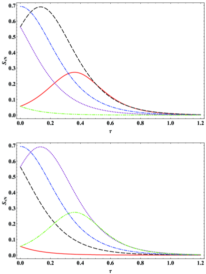
Figure 1: Entropy $S_{\rm vN}$ (33) versus $\tau$ for the values of $\tilde{\gamma}=-2$ (top plot) and $\tilde{\gamma}=2$ (bottom plot), at the different values of $p$: $0.01$ (solid line), $1/4$ (dashed line), $1/2$ (dash-dotted line), $3/4$ (dotted line) and $0.99$ (dash-double-dotted line).

As an initial state we choose the superposition of the ground and excited states

$$\hat{\rho}(0)=\hat{\Omega}(0)=p\left|e\right\rangle\left\langle e\right|+(1-p)\left|g\right\rangle\left\langle g\right|=\begin{pmatrix}p&0\\ 0&1-p\end{pmatrix},$$ (27)

where $0\leqslant p\leqslant 1$ is a free parameter. It is easy to check that this state is pure at $p=0,\,1$ and mixed otherwise. Solving the evolution equations (5), with the initial condition (27), we obtain the following expression for the non-normalized density operator

$$\hat{\Omega}=\frac{1}{2\mu^{2}}\left[2f_{y}(t)\hat{\sigma}_{y}+f_{z}(t)\hat{\sigma}_{z}+F(t)\hat{I}\right],$$ (28)

where we denoted:

$$f_{y}(t)=\sinh{(\mu\tau)}\left[\mu\bar{p}\cosh{(\mu\tau)}-\tilde{\gamma}\sinh{(\mu\tau)}\right],$$ (29)

$$f_{z}(t)=\mu\left[\mu\bar{p}\cosh{(2\mu\tau)}-\tilde{\gamma}\sinh{(2\mu\tau)}\right],$$ (30)

$$F(t)=\tilde{\gamma}^{2}\cosh{(2\mu\tau)}-\mu\bar{p}\tilde{\gamma}\sinh{(2\mu\tau)}-1,$$ (31)

where $\tau=\Delta t$, $\tilde{\gamma}=\gamma/\Delta$, $\bar{p}=2p-1$, and the value $\mu=\sqrt{\tilde{\gamma}^{2}-1}$ is assumed to be positive throughout the paper. One can see that for the chosen initial state (27), $\text{Tr}\,\hat{\Omega}$ is invariant under the simultaneous transformation $\tilde{\gamma}\to-\tilde{\gamma}$ and $p\to 1-p$, which will manifest itself in the behavior of $S_{\text{NH}}$ below. Consequently, the normalized density matrix is given by:

$$\hat{\rho}=\frac{f_{y}(t)}{F(t)}\hat{\sigma}_{y}+\frac{f_{z}(t)}{2F(t)}\hat{\sigma}_{z}+\frac{1}{2}\hat{I}.$$ (32)

The von Neumann entropy can be computed directly from the definition (12). It is given by (in units where $k_{B}=1$):

$$S_{\rm vN}=-F_{+}^{(2)}(t)\,\text{ln}F_{+}^{(1)}(t)-F_{-}^{(2)}(t)\,\text{ln}F_{-}^{(1)}(t),$$ (33)

where we denoted $F_{\pm}^{(i)}(t)=\tfrac{1}{2}\left[1\pm\sqrt{F_{i}(t)}/F(t)\right]$, $i=1,2$, and

$$F_{1}(t) = 4\,\text{sinh}^{2}\!\left(\mu\tau\right)\left[\mu\bar{p}\cosh{(\mu\tau)}-\tilde{\gamma}\sinh{(\mu\tau)}\right]^{2}+\mu^{2}\left[\mu\bar{p}\cosh{(2\mu\tau)}-\tilde{\gamma}\sinh{(2\mu\tau)}\right]^{2},$$ (34)

$$F_{2}(t) = \mu\bar{p}\tilde{\gamma}\left[2\sinh{(2\mu\tau)}-\tilde{\gamma}^{2}\sinh{(4\mu\tau)}\right]+\frac{1}{2}\tilde{\gamma}^{2}\left[(\mu^{2}(\bar{p}^{2}+1)+1)\cosh{(4\mu\tau)}-4\cosh{(2\mu\tau)}\right]$$ (35)

$$+\frac{1}{2}\left[\mu^{4}(\bar{p}^{2}-1)-\mu^{2}(\bar{p}^{2}-2)+3\right].$$

The typical profiles of the entropy (33) for the initial state (27) are shown in Fig. 1. One can see that the entropy $S_{\rm vN}$ tends to zero at large times, regardless of the sign of $\tilde{\gamma}$.

The NH entropy, defined in Eq. (14), can be computed using the relation (16). It turns out to be (in units where $k_{B}=1$):

$$S_{\text{NH}}=S_{\rm vN}-\ln{\left[F(t)/\mu^{2}\right]},$$ (36)

where $S_{\rm vN}$ is given by (33). One can see that if the von Neumann entropy remains finite at large times then the asymptotical properties of $S_{\text{NH}}$ are determined by the behavior of $F(t)$, i.e.,

$$\lim\limits_{t\to\infty}S_{\text{NH}}=\ln{\mu^{2}}-\lim\limits_{t\to\infty}\ln{F(t)}\propto-2\mu\tau,$$ (37)

such that $S_{\text{NH}}$ tends to a linear function at large times.

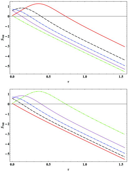
Figure 2: Entropy $S_{\text{NH}}$ (36) versus $\tau$ for the values of $\tilde{\gamma}=-2$ (top plot) and $\tilde{\gamma}=2$ (bottom plot), at the different values of $p$: $0.01$ (solid line), $1/4$ (dashed line), $1/2$ (dash-dotted line), $3/4$ (dotted line) and $0.99$ (dash-double-dotted line).

The profiles of the entropy (36) for the initial state (27) are shown in Fig. 2. One can see that the entropy decreases with time, regardless of the sign of $\tilde{\gamma}$, as one can expect from equations (31) and (36). It is instructive to compare this with the plots for the trace of the non-normalized density matrix, shown in Fig. 3, which indicate the flow rate of probability to/from the system. For this model, the entropy $S_{\text{NH}}$ takes negative values at large times. This will be discussed in details in the concluding section.

IV.3 Two-level tunneling model with non-Hermitian detuning and asymptotically constant NH entropy

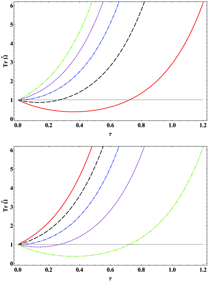
Figure 3: Profiles of $\text{Tr}\,\hat{\Omega}$, where $\hat{\Omega}$ is given by (28), versus $\tau$ for the values of $\tilde{\gamma}=-2$ (top plot) and $\tilde{\gamma}=2$ (bottom plot), at the different values of $p$: $0.01$ (solid line), $1/4$ (dashed line), $1/2$ (dash-dotted line), $3/4$ (dotted line) and $0.99$ (dash-double-dotted line).

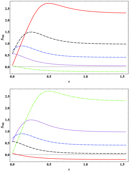
Figure 4: Entropy $S_{\text{NH}}$ (40) versus $\tau$ for the values of $\tilde{\gamma}=-2$ (top plot) and $\tilde{\gamma}=2$ (bottom plot), at the different values of $p$: $0.01$ (solid line), $1/4$ (dashed line), $1/2$ (dash-dotted line), $3/4$ (dotted line) and $0.99$ (dash-double-dotted line).

For the previous two-level model we found out that the NH entropy goes to negative values during time evolution. Here we illustrate that this behavior can be changed just by adding a constant decay operator to the $\hat{\Gamma}$ operator, as explained in the last paragraphs of section III.

Thus, the Hermitian part of the model is given by (25) whereas the $\hat{\Gamma}$ operator is (in units $k_{B}=1$):

$$\hat{\Gamma}=\hbar\gamma\hat{\sigma}_{z}+\hbar\mu\hat{I}.$$ (38)

Unless otherwise specified, here and in the following, we assume the notation of section IV.2. The initial conditions for the evolution equation remain (27).

Using the results given in the Appendix, one can easily show that, for this model, both the normalized density $\hat{\rho}$ and von Neumann entropy $S_{\text{vN}}$ are the same as those obtained for the model in Sec. IV.2. However, the operator (28) acquires the factor $\exp{(-2\mu t)}$:

$$\hat{\Omega}=\frac{1}{2\mu^{2}}\text{e}^{-2\mu t}\left[2f_{y}(t)\hat{\sigma}_{y}+f_{z}(t)\hat{\sigma}_{z}+F(t)\hat{I}\right].$$ (39)

Therefore, using the transformations in Eq. (17), we obtain

$$S_{\text{NH}}=S_{\rm vN}-\ln{\left[F(t)/\mu^{2}\right]}+2\mu\tau,$$ (40)

where $S_{\rm vN}$ is given by (33). The asymptotical value is given by

$$\lim\limits_{t\to+\infty}S_{\text{NH}}=\ln{\left[\frac{2\mu^{2}}{\tilde{\gamma}(\tilde{\gamma}-\mu\bar{p})}\right]}.$$ (41)

Unlike its analogue in Sec. IV.2, the $S_{\text{NH}}$ entropy for this model is bounded. As a matter of fact, considering the more general form of the $\hat{\Gamma}$ operator, $\hat{\Gamma}=\hbar\gamma\hat{\sigma}_{z}+k\hbar\mu\hat{I}$ (where $k$ is an arbitrary real number), one can establish that the value $k=1$ acts as a critical threshold: the NH entropy decreases asymptotically if $k<1$ (see the model in Sec. IV.2), while it increases if $k>1$ (see the model in Sec. IV.4).

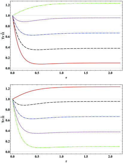
Figure 5: Profiles of $\text{Tr}\,\hat{\Omega}$, where $\hat{\Omega}$ is given by (39), versus $\tau$, for the values of $\tilde{\gamma}=-2$ (top plot) and $\tilde{\gamma}=2$ (bottom plot), at the different values of $p$: $0.01$ (solid line), $1/4$ (dashed line), $1/2$ (dash-dotted line), $3/4$ (dotted line) and $0.99$ (dash-double-dotted line).

The profiles of the von Neumann entropy, the NH entropy and the trace of the operator $\hat{\Omega}$ for this model are shown in Figs. 1, 4 and 5, respectively. On can see that, as for the model in Sec. IV.2, the entropy $S_{\text{NH}}$ may takes negative values for a certain range of parameters (when the trace of $\hat{\Omega}$ goes above one). This will be discussed in details in the concluding section.

IV.4 Two-level tunneling model with non-Hermitian detuning and increasing NH entropy

In the two previous cases, we found that the NH entropy can assume a negative infinite value or a constant value. Here we consider another model that, instead, provides an entropy that asymptotically increases with time. Also in this case, such a behavior can achieved just by adding a constant term to the $\hat{\Gamma}$ operator, as explained in the last paragraphs of section III.

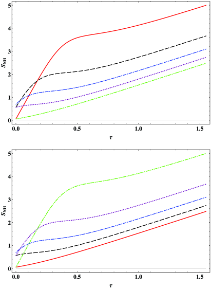
Figure 6: Entropy $S_{\text{NH}}$ (44) versus $\tau$ for the values of $\tilde{\gamma}=-2$ (top plot) and $\tilde{\gamma}=2$ (bottom plot), at the different values of $p$: $0.01$ (solid line), $1/4$ (dashed line), $1/2$ (dash-dotted line), $3/4$ (dotted line) and $0.99$ (dash-double-dotted line).

The Hermitian part of this model is still given by Eq. (25) whereas the $\hat{\Gamma}$ operator is (in units $k_{B}=1$):

$$\hat{\Gamma}=\hbar\gamma\hat{\sigma}_{z}+\frac{3}{2}\hbar\mu\hat{I}.$$ (42)

As one can see, the constant term multiplying the identity operator in the definition of $\hat{\Gamma}$ above is $\tfrac{3}{2}\hbar\mu$. Although, this case is qualitatively similar to any other one with the constant term’s coefficient larger than $\hbar\mu$. The initial conditions for the evolution equation remain (27).

Using the results given in the Appendix, one can easily show that for this model both the normalized density $\hat{\rho}$ and von Neumann entropy $S_{\text{vN}}$ are the same as for the models in Secs. IV.2 and IV.3, whereas the operator (28) acquires the factor $\exp{(-3\mu t)}$:

$$\hat{\Omega}=\frac{1}{2\mu^{2}}\text{e}^{-3\mu t}\left[2f_{y}(t)\hat{\sigma}_{y}+f_{z}(t)\hat{\sigma}_{z}+F(t)\hat{I}\right].$$ (43)

Therefore, using (17), we obtain

$$S_{\text{NH}}=S_{\rm vN}-\ln{\left[F(t)/\mu^{2}\right]}+3\mu\tau,$$ (44)

where $S_{\rm vN}$ is given by (33). The asymptotical value is given by

$$\lim\limits_{t\to+\infty}S_{\text{NH}}=\ln{\mu^{2}}-\lim\limits_{t\to\infty}\ln{F(t)}+3\mu\tau\propto\mu\tau,$$ (45)

such that $S_{\text{NH}}$ tends to a linear function with a positive coefficient at large times.

The profiles of the von Neumann entropy, NH entropy and the trace of the operator $\hat{\Omega}$ for this model are shown in Figs. 1, 6 and 7, respectively.

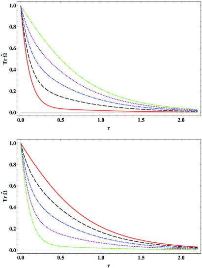
Figure 7: Profiles of $\text{Tr}\,\hat{\Omega}$, where $\hat{\Omega}$ is given by (43), versus $\tau$, for the values of $\tilde{\gamma}=-2$ (top plot) and $\tilde{\gamma}=2$ (bottom plot), at the different values of $p$: $0.01$ (solid line), $1/4$ (dashed line), $1/2$ (dash-dotted line), $3/4$ (dotted line) and $0.99$ (dash-double-dotted line).

V Discussion and conclusions

In this paper we have provided a generalized formulation of the quantum fine-grained entropy for systems described by non-Hermitian Hamiltonians. We have adopted a straightforward generalization of the von Neumann entropy, defined in terms of the normalized density matrix (obeying a nonlinear equation of motion), and introduced another definition of an entropy, $S_{\rm NH}$, in terms of the normalized average of the logarithm of the non-normalized density matrix. We have shown that in both cases the entropy production is non-zero. However, we have found that it is $S_{\rm NH}$ that properly captures the physical behavior of the probability and disorder in a system in presence of sinks or sources described by non-Hermitian Hamiltonians.

In Sec. IV we have studied some models in order to illustrate the different behavior of the $S_{\rm vN}$ and $S_{\rm NH}$ entropies. In particular, for the models in Secs. IV.2-IV.4 both the normalized density operator, $\hat{\rho}$, and the von Neumann entropy, $S_{\text{vN}}$, do not change while the entropy $S_{\rm NH}$ does. We show that at large times the value $S_{\rm NH}$ decreases asymptotically for the model of Sec. IV.2, it tends to a finite value for the model in Sec. IV.3, and it increases for the model in Sec. IV.4.

The results of the present work, when considered together with our previous studies sz14 ; ks ; sz14cor , allow us to draw a certain number of conclusions. Non-Hermitian dynamics is able to describe in the quantum realm the production of entropy in a way similar to what non-Hamiltonian dynamics with phase space compressibility does in the classical realm. Non-Hermitian dynamics also seems to need both the normalized density operator, $\hat{\rho}$, and non-normalized one, $\hat{\Omega}$, in order to provide a proper statistical theory. The non-normalized density operator, defined as a solution of Eq. (5), captures some important features of the decay process, such as the non-conservation of probability in the (sub)system and its “leakage” into the surrounding environment. The normalized density operator guarantees that the probabilistic interpretation of averages can be maintained. In this regard, the entropy $S_{\text{NH}}$ combines both operators in a proper way and can signal the expected thermodynamic behavior of an open system. The entropy $S_{\text{NH}}$ also seems more suitable for describing the gain-loss processes that are related to the probability’s non-conservation, since it contains information not only about the conventional von Neumann entropy $S_{\text{vN}}$ but also about the trace of the operator $\hat{\Omega}$, according to the relation (16). Assuming that $S_{\text{vN}}$ is bound at large times, the NH entropy grows when $\text{Tr}\,\hat{\Omega}$ decreases, also it takes positive values if $\text{Tr}\,\hat{\Omega}<1$ and negative ones otherwise. Hence, one can say that $S_{\text{NH}}$ describes the flow of information between the system and the bath.

Further studies are needed to understand whether and when $S_{\rm NH}$ may deserve a complete quantitative thermodynamic status as well as whether there might be viable physical interpretations of a negative entropy (not necessarily given in terms of the number of occupied microscopic states).

Appendix A Hamiltonian shift transformations and entropy

Following the discussions presented in Refs. sz14 ; ks , let us consider the following transformation of the $\hat{\Gamma}$ operator

$$\hat{\Gamma}=\hat{\Gamma}^{\prime}+\frac{1}{2}\hbar\alpha\hat{I},$$ (46)

where $\alpha$ is an arbitrary real constant and $\hat{I}$ is the unity operator. This transformation is a subset of the transformation

$$\hat{\cal H}=\hat{\cal H}^{\prime}+c_{0}\hat{I},$$ (47)

$c_{0}$ being an arbitrary complex number, which is the non-Hermitian generalization of the energy shift in conventional quantum mechanics. Therefore, in Refs. sz14 ; ks it was called the “gauge” transformation of the Hamiltonian (1), whereas the terms of the type $c_{0}\hat{I}$ can be called the “gauge” terms.

In Ref. ks it was shown that the equation (8) is invariant under the transformation (46), therefore, one immediately obtains

$$\hat{\rho}=\hat{\rho}^{\prime},\ S_{\text{vN}}=S_{\text{vN}}^{\prime},$$ (48)

therefore the von Neumann entropy is not affected by the transformation (46). One can see that any information regarding the shifting of the total non-Hermitian Hamiltonian is lost if one deals solely with the normalized density operator.

However, the evolution equation (6) is not invariant under the shift (46). If $\hat{\cal H}$ is time-independent then, substituting (46) into (6), we obtain that the non-normalized density acquires an exponential factor:

$$\hat{\Omega}=\hat{\Omega}^{\prime}\exp{(-\alpha t)},$$ (49)

therefore, recalling the relation (16), we obtain

$$S_{\text{NH}}=S_{\text{vN}}^{\prime}-k_{B}\ln{\text{Tr}\,\hat{\Omega}}=S_{\text{NH}}^{\prime}+k_{B}\alpha t,$$ (50)

which indicates that any lost information about the shifting term in Eq. (47) in the total non-Hermitian Hamiltonian, due the normalization procedure in Eq. (7), can be recovered by means of the NH entropy.

References

- (1) H. B. Callen, Thermodynamics and an Introduction to Thermostatistics (John Wiley & Sons, New York, 1985).
- (2) Y. Aharonov and D. Rohrlich, Quantum Paradoxes (Wiley-VCH, Weinheim, 2005).
- (3) R. Balescu, Equilibrium and Nonequilibrium Statistical Mechanics (John Wiley & Sons, New York, 1975).
- (4) S. Nosè, Mol. Phys. 52, 255 (1984).
- (5) W. G. Hoover, Phys. Rev. A 31, 1695 (1985).
- (6) A. Sergi and M. Ferrario, Phys. Rev. E 64, 056125 (2001).
- (7) A. Sergi, Phys. Rev. E 67, 021101 (2003).
- (8) A. Sergi and P. V. Giaquinta, J. Stat. Mech. Theory and Exp. 02, P02013 (2007).
- (9) L. Andrey, Phys. Lett. A 111, 45 (1985).
- (10) L. Andrey, Phys. Lett. A 114, 183 (1986).
- (11) C. E. Rüter, K. G. Makris, R. El-Ganainy, D. N. Christodoulides, M. Segev, and D. Kip, Nature Phys. 6, 192 (2010).
- (12) A. Guo, G. J. Salamo, D. Duchesne, R. Morandotti, M. Volatier-Ravat, V. Aimez, G. A. Siviloglou, and D. N. Christodoulides, Phys. Rev. Lett. 103, 093902 (2009).
- (13) N. Moiseyev, Phys. Rep. 302, 211 (1998).
- (14) W. John, B. Milek, H. Schanz, and P. Seba, Phys. Rev. Lett. 67, 1949 (1991).
- (15) C. A. Nicolaides and S. I. Themelis, Phys. Rev. A 45, 349 (1992).
- (16) H. Feshbach, Ann. Phys. 5, 357 (1958).
- (17) H. Feshbach, Ann. Phys. 19, 287 (1962).
- (18) E. C. G. Sudarshan, Phys. Rev. D 18, 2914 (1978).
- (19) S. Selstø, T. Birkeland, S. Kvaal, R. Nepstad, and M. Førre, J. Phys. B: At. Mol. Opt. Phys. 44, 215003 (2011).
- (20) H. C. Baker, Phys. Rev. Lett. 50, 1579 (1983).
- (21) H. C. Baker, Phys. Rev. A 30, 773 (1984).
- (22) S.-I. Chu and W. P. Reinhardt, Phys. Rev. Lett. 39, 1195 (1977).
- (23) J. Korringa, Phys. Rev. 133, 1228 (1964).
- (24) J. Wong, J. Math. Phys. 8, 2039 (1967).
- (25) G. C. Hegerfeldt, Phys. Rev. A 47, 449 (1993).
- (26) S. Baskoutas, A. Jannussis, R. Mignani, and V. Papatheou, J. Phys. A 26, L819 (1993).
- (27) P. Angelopoulou, S. Baskoutas, A. Jannussis, R. Mignani, and V. Papatheou, Int. J. Mod. Phys. B 9, 2083 (1995).
- (28) I. Rotter, arXiv:0711.2926.
- (29) I. Rotter, J. Phys. A 42, 153001 (2009).
- (30) H. B. Geyer, F. G. Scholtz and K. G. Zloshchastiev, in: Proceedings of International Conference on Mathematical Methods in Electromagnetic Theory (Odessa, 2008) pp. 250-252.
- (31) R. Lo Franco, B. Bellomo, S. Maniscalco, and G. Compagno, Int. J. Mod. Phys. B 27, 1345053 (2013).
- (32) S. Banerjee and R. Srikanth, Mod. Phys. Lett. B 24, 2485 (2010).
- (33) F. Reiter and A. S. Sørensen, Phys. Rev. A 85, 032111 (2012).
- (34) D. C. Brody and E.-M. Graefe, Phys. Rev. Lett. 109, 230405 (2012).
- (35) K. G. Zloshchastiev and A. Sergi, J. Mod. Optics 61, 1298 (2014).
- (36) A. Sergi and K. Zloshchastiev, Int. J. Mod. Phys. B 27, 1350163 (2013).
- (37) J. von Neumann, The Mathemathical Foundation of Quantum Mechanics (Princeton University Press, Princeton, 1955).
- (38) H.-P. Breuer and F. Petruccione, The Theory of Open Quantum Systems (Oxford University Press, 2002).
- (39) E.-M. Graefe, M. Höning, and H. J. Korsch, J. Phys. A 43, 075306 (2010).
- (40) M. Znojil, J. Nonlin. Math. Phys. 9, 122-133 (2002).
- (41) A. Sergi and K. Zloshchastiev, Phys. Rev. A 91, 062108 (2015).
- (42) R. N. Oerter, Am. J. Phys. 79, 297 (2011).
- (43) R. Balian, Am. J. Phys. 67, 1078 (1999).
- (44) A. J. Leggett, et al., Rev. Mod. Phys. 59, 1 (1987).
- (45) F. G. Scholtz, H. B. Geyer and F. J. W. Hahne, Ann. Phys. 213, 74 (1992).
- (46) C. M. Bender and S. Boettcher, Phys. Rev. Lett. 80, 5243 (1998).