A model independent method for quantitative estimation of $S\!U(3)$ flavor symmetry breaking using Dalitz plot

Abstract

The light hadron states are satisfactorily described in the quark model using $S\!U(3)$ flavor symmetry. If the $S\!U(3)$ flavor symmetry relating the light hadrons were exact, one would have an exchange symmetry between these hadrons arising out of the exchange of the up, down and strange quarks. This aspect of $S\!U(3)$ symmetry is used extensively to relate many decay modes of heavy quarks. However, the nature of the effects of $S\!U(3)$ breaking in such decays is not well understood and hence, a reliable estimate of $S\!U(3)$ breaking effects is missing. In this work we propose a new method to quantitatively estimate the extent of flavor symmetry breaking and better understand the nature of such breaking using Dalitz plot. We study the three non-commuting $S\!U(2)$ symmetries (subsumed in $S\!U(3)$ flavor symmetry): isospin (or $T$-spin), $U$-spin and $V$-spin, using the Dalitz plots of some three-body meson decays. We look at the Dalitz plot distributions of decays in which pairs of the final three particles are related by two distinct $S\!U(2)$ symmetries. We show that such decay modes have characteristic distributions that enable the measurement of violation of each of the three $S\!U(2)$ symmetries via Dalitz plot asymmetries in a single decay mode. Experimental estimates of these easily measurable asymmetries would help in better understanding the weak decays of heavy mesons into both two and three light mesons.

I Introduction

A satisfactory understanding of the light hadronic states using $S\!U(3)$ flavor symmetry is one of the outstanding success stories of particle physics GellMann:1961 ; GellMann:1962xb ; Ne'eman:1961cd ; Okubo:1961jc ; Okubo:1964xz . In its true essence the $S\!U(3)$ flavor symmetry denotes the full exchange symmetry amongst the up ($u$), down ($d$) and strange ($s$) quarks. Another implication of $S\!U(3)$ flavor symmetry, if it were an exact symmetry, is that the mesons formed by combining the quarks $u$, $d$, $s$ and the antiquarks $\bar{u}$, $\bar{d}$, $\bar{s}$ belonging to the same representation of $S\!U(3)$ would also be degenerate. One treats the three quarks on the same footing even though the quark masses differ by allowing for a breaking of the symmetry. The success of the Gell-Mann-Okubo mass formula in relating the hadron masses is that it takes the small $S\!U(3)$ breaking into account but does not depend on the details of $S\!U(3)$ breaking effects. Such $S\!U(3)$ breaking effects cannot be calculated and must be estimated using experimental inputs. Traditionally, the mass differences between these mesons have been used as a measure of the extent of breaking of $S\!U(3)$ flavor symmetry. The masses of these mesons, which are bound states of quark-antiquark pairs, depend on their binding energies. It is not possible to estimate these binding energies from QCD calculations since these resonances lie in the non-relativistic low energy regime. Moreover, the electro-magnetic interactions between the quark and the antiquark in the meson also contribute towards its binding energy. Thus, by measuring the mass differences amongst the mesons one does not fully solicit the breaking of $S\!U(3)$ flavor symmetry. Another usual way to explore the breaking $S\!U(3)$ flavor symmetry is to look at specific loop diagrams where the down and strange quarks contribute. The loop effects affect the amplitude of the process under consideration and its physical manifestations are then studied for a quantitative estimation of the breaking of $S\!U(3)$ flavor symmetry. Since up quark has different electric charge than down and strange, it can not be treated in the same way in these studies of loop contributions. Therefore, such a method also fails to probe the full exchange symmetry of these three light quarks. Hence, all estimates of $S\!U(3)$ breaking are currently empirical.

Several studies exist in literature that have used broken $S\!U(3)$ flavor symmetry (i) in various decay modes using the methods of amplitudes (usually isospin and $U$-spin amplitudes) and various quark diagrams  Kingsley:1975fe ; Voloshin:1975yx ; Wang:1979dx ; Quigg:1979ic ; Zeppenfeld:1980ex ; Chau:1986du ; Chau:1987tk ; Savage:1989ub ; Chau:1990ay ; Savage:1991wu ; Lipkin:1991st ; Chau:1991gx ; Kwong:1993ri ; Hinchliffe:1995hz ; Gronau:1995hm ; Oh:1998wa ; Rosner:1999xd ; Gronau:2000ru ; Deshpande:2000jp ; Wu:2002nz ; Khodjamirian:2003xk ; Chiang:2003pm ; Zhong:2004ck ; Chiang:2004nm ; Wu:2004ht ; Wu:2005hi ; Gronau:2005ax ; Chiang:2006ih ; Soni:2006vi ; Chiang:2007bd ; Chiang:2007qh ; Bhattacharya:2008ss ; Chiang:2008zb ; Wei:2009zzh ; Jung:2009pb ; Imbeault:2011jz ; Cheng:2011qh ; Pirtskhalava:2011va ; Cheng:2012xb ; Pham:2012db ; Hiller:2012xm ; Bhattacharya:2014eca ; Cheng:2014rfa ; Pham:2014lla ; He:2014xha ; Ledwig:2014rfa ; Gronau:2015rda , and (ii) in determinations of weak phases and $C\!P$ violating phases Kim:1998sh ; Gronau:1998rr ; Datta:2003va ; Gronau:2005pq ; Gronau:2006gn ; Gronau:2007af ; Calibbi:2009pv ; ReyLeLorier:2011ww ; He:2013vta ; Bhattacharya:2013cla ; Grossman:2013lya ; Fong:2013dnk . These methods involve comparison of observables in distinct decay modes which are related by some underlying $S\!U(2)$ symmetries, such as isospin, $U$-spin or $V$-spin. However, the full exchange symmetry amongst the three light quarks has not yet been fully exploited, in a single decay mode. Hadronic weak decays involve several unknown parameters which can be reduced by the use of $S\!U(3)$ flavor symmetry. Since, $S\!U(3)$ flavor symmetry is still extensively used to relate the few decay modes of heavy quarks, it is important to realize other ways to experimentally measure the breaking of $S\!U(3)$ flavor symmetry and understand better the complete nature of $S\!U(3)$ breaking. In this paper we propose a method to achieve precisely this by looking at asymmetries in the Dalitz plot under exchange of the mesons in the final state. These asymmetries can be measured in different regions of the Dalitz plot. In particular these asymmetries can be measured both along resonances and in the non-resonant regions. A quantitative estimate of the variation of these asymmetries obtained experimentally would provide valuable understanding of $S\!U(3)$ breaking effects. It would also be interesting to find regions of the Dalitz plots where $S\!U(3)$ is a good symmetry. The $S\!U(3)$ flavor symmetry subsumes three important and non-commuting $S\!U(2)$ symmetries: isospin (or $T$-spin), $U$-spin and $V$-spin. All the members of a $S\!U(3)$ multiplet are related to one another by combined operations of the raising and lowering operators of these individual $S\!U(2)$ symmetries. In this paper we restrict ourselves to the breaking of these $S\!U(2)$ symmetries in combinations.

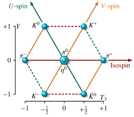
Figure 1: The $S\!U(3)$ meson octet of light pseudo-scalar mesons. Here the horizontal axis shows the eigenvalues of isospin ($T_{3}$) and the vertical axis shows the eigenvalues of hypercharge ($Y=B+S$, with $B$ being baryon number and $S$ being the strangeness number). The dotted lines parallel to $U$-spin (or isospin) axis signify that in no two-body decays of $B$ or $D$ meson can the two connected mesons appear together in the final state as that would violate conservation of electric charge (or strangeness by two units).

We shall work with the three-body decays of the type $P\to M_{1}M_{2}M_{3}$, where $P$ can be either a $B$ or a $D$ meson and the final particles $M_{1}$, $M_{2}$ and $M_{3}$ are distinct members of the lightest pseudo-scalar $S\!U(3)$ multiplet (see Fig. 1). Our approach towards experimental estimation of breaking of $S\!U(3)$ flavor symmetry, primarily looks for violations of two constituent $S\!U(2)$ symmetries. Therefore, our final state would have a pair of particles in one $S\!U(2)$ multiplet and another pair belonging to a different $S\!U(2)$ multiplet. If the $S\!U(2)$ symmetry is assumed to be exact, the pairs of final state particles that are members of the $S\!U(2)$ multiplet are identical bosons in the symmetry limit and must be totally symmetric under exchange. This implies that if the wave-function is symmetric under $S\!U(2)$ exchange it must be even under space exchange, whereas if it is anti-symmetric in $S\!U(2)$, it must be odd under space exchange too. We shall explicitly explore this exchange symmetry to deduce some simple relations that predict a pattern in the distribution of events in the concerned Dalitz plot. Any deviation from this predicted Dalitz plot distribution would, therefore, constitute a test of breaking of $S\!U(3)$ flavor symmetry. Dalitz plots have previously been used in Refs. Sinha:2011ky ; Sahoo:2013mqa ; Sahoo:2014nna to extract weak decay amplitudes and to study $C\!P$, $C\!PT$ and Bose symmetry violations. Here we use the Dalitz plot to look for breaking of $S\!U(3)$ flavor symmetry in a single decay mode.

We start Sec.II by explaining briefly in subsection II.1 the kind of Dalitz plot we shall use to elucidate our method and also set up the notation to be followed thenceforth. We shall then illustrate the method in full detail in subsection II.2 by considering the decay mode $B^{+}\to K^{0}\pi^{0}\pi^{+}$ which tests both isospin and $U$-spin simultaneously. We show in detail how the exchange $\pi^{0}\leftrightarrow\pi^{+}$ under isospin and $K^{0}\leftrightarrow\pi^{0}$ under $U$-spin results in a characteristic distribution of events in the Dalitz plot if both isospin and $U$-spin are exact symmetries. The method can equally well be applied to the decay mode $D^{+}_{s}\to K^{0}\pi^{0}\pi^{+}$. We then show how $G$-parity generalized to $V$-spin further influences the distribution of events in the Dalitz plot. The definition of $G$-parity and its generalization to $U$-spin and $V$-spin are discussed in the Appendix A for ready reference. We provide Dalitz plot asymmetries which can then be easily used to make quantitative estimate of the breaking of $S\!U(3)$ flavor symmetry. Then, we sketch out the necessary steps for handling cases of both isospin and $V$-spin violation (in subsection II.3) as well as both $U$-spin and $V$-spin violation (in subsection II.4) by considering the decay modes $B^{0}_{d}\text{ or }\kern 1.79993pt\bar{\kern-1.79993ptB}{}^{0}_{s}\to K^{+}\pi^{0}\pi^{-}$ and $B^{+}\text{ or }D^{+}\to K^{+}\pi^{0}\kern 1.99997pt\bar{\kern-1.99997ptK}{}^{0}$ respectively. Finally in subsection II.5, we sketch out as to how our method can be applied to a decay mode $D^{+}\to\pi^{+}\pi^{0}\kern 1.99997pt\bar{\kern-1.99997ptK}{}^{0}$ where each pair of particles in the final state can be directly related by one of the three $S\!U(2)$ symmetries, namely isospin, $U$-spin and $V$-spin. We point out how the Dalitz plot distribution for this mode differs from the ones considered in the earlier subsections. Finally, we conclude in section III emphasizing the salient features of our method.

II The method

Final state			Kind of $S\!U(2)$ exchange		Expression for the state
$M_{1}$	$M_{2}$	$M_{3}$	$M_{1}\leftrightarrow M_{2}$	$M_{2}\leftrightarrow M_{3}$	$\left|M_{1}M_{2}\right\rangle$	$\left|M_{2}M_{3}\right\rangle$
$K^{0}$	$\pi^{0}$	$\pi^{+}$	$U$-spin	Isospin	$\frac{1}{2\sqrt{2}}\Big{(}\left|2,+1\right\rangle_{U}+\left|1,+1\right\rangle_{U}\Big{)}-\frac{\sqrt{3}}{2}\left|1^{\prime},+1\right\rangle_{U}$	$-\frac{1}{\sqrt{2}}\Big{(}\left|2,+1\right\rangle_{I}-\left|1,+1\right\rangle_{I}\Big{)}$
$K^{+}$	$\pi^{0}$	$\pi^{-}$	$V$-spin	Isospin	$-\frac{1}{2\sqrt{2}}\Big{(}\left|2,+1\right\rangle_{V}+\left|1,+1\right\rangle_{V}\Big{)}+\frac{\sqrt{3}}{2}\left|1^{\prime},+1\right\rangle_{V}$	$\frac{1}{\sqrt{2}}\Big{(}\left|2,-1\right\rangle_{I}+\left|1,-1\right\rangle_{I}\Big{)}$
$K^{+}$	$\pi^{0}$	$\kern 1.99997pt\bar{\kern-1.99997ptK}{}^{0}$	$V$-spin	$U$-spin	$-\frac{1}{2\sqrt{2}}\Big{(}\left|2,+1\right\rangle_{V}+\left|1,+1\right\rangle_{V}\Big{)}+\frac{\sqrt{3}}{2}\left|1^{\prime},+1\right\rangle_{V}$	$\frac{1}{2\sqrt{2}}\Big{(}\left|2,-1\right\rangle_{U}+\left|1,-1\right\rangle_{U}\Big{)}-\frac{\sqrt{3}}{2}\left|1^{\prime},-1\right\rangle_{U}$
$\pi^{+}$	$\pi^{0}$	$\kern 1.99997pt\bar{\kern-1.99997ptK}{}^{0}$	Isospin	$U$-spin	$-\frac{1}{\sqrt{2}}\Big{(}\left|2,+1\right\rangle_{I}+\left|1,+1\right\rangle_{I}\Big{)}$	$-\frac{1}{2\sqrt{2}}\Big{(}\left|2,-1\right\rangle_{U}+\left|1,-1\right\rangle_{U}\Big{)}+\frac{\sqrt{3}}{2}\left|1^{\prime},-1\right\rangle_{U}$

Table 1: We look at decays with the final states $M_{1}M_{2}M_{3}$ given as in the table here. The particle $M_{2}$, which is always $\pi^{0}$, being at the center of the pseudoscalar meson octet belongs to all the three $S\!U(2)$ symmetries under consideration. The states are denoted with subscripts for clarity, e.g. the state $\left|U=1,U_{3}=+1\right\rangle$ is denoted as $\left|1,+1\right\rangle_{U}$. Modes with conjugate final states can as well be studied in a similar manner. The primed states such as $\left|1^{\prime},\pm 1\right\rangle$ arise from the $\left|0,0\right\rangle$ component of $\pi^{0}$ under $U$-spin and $V$-spin considerations as discussed in the text. The last mode in the table with final state $\pi^{+}\pi^{0}\kern 1.99997pt\bar{\kern-1.99997ptK}{}^{0}$ has another exchange symmetry, namely exchange of $\pi^{+}$ and $\kern 1.99997pt\bar{\kern-1.99997ptK}{}^{0}$ under $V$-spin. Thus $\left|\pi^{+}\kern 1.99997pt\bar{\kern-1.99997ptK}{}^{0}\right\rangle=\frac{1}{\sqrt{2}}\Big{(}\left|1,0\right\rangle_{V}+\left|0,0\right\rangle_{V}\Big{)}$ under $V$-spin.

II.1 General considerations

The method described in this paper relies on the simultaneous application of two of the $S\!U(2)$ symmetries subsumed in $S\!U(3)$ i.e. isospin (or $T$-spin), $U$-spin or $V$-spin, to a three body decay $P\to M_{1}M_{2}M_{3}$, where $M_{1}$, $M_{2}$ and $M_{3}$ are chosen such that $M_{1}$ and $M_{2}$ belong to the triplet of one of the $S\!U(2)$ subgroups and $M_{2}$ and $M_{3}$ belongs to another. To be definite $M_{2}$ is always chosen to be the $\pi^{0}$ and the modes we consider are listed in Table 1. Under the limit of exact $S\!U(2)$ all the meson belonging to the triplet are identical bosons and must exhibit an overall Bose symmetry under exchange. This behavior must also be reflected in the Dalitz plot for the decay. We can construct a Dalitz plot out of the Mandelstam-like variables $s$, $t$ and $u$. Let us denote the 4-momenta of particles $P$ and $M_{i}$ (where $i\in\{1,2,3\}$) by $p$ and $p_{i}$ and their masses by $m$ and $m_{i}$ respectively. The variables $s,t,u$ are defined in terms of the 4-momenta as follows:

$$s =\left(p-p_{1}\right)^{2}=\left(p_{2}+p_{3}\right)^{2},$$ (1)

$$t =\left(p-p_{2}\right)^{2}=\left(p_{1}+p_{3}\right)^{2},$$

$$u =\left(p-p_{3}\right)^{2}=\left(p_{1}+p_{2}\right)^{2}.$$

It is easy to observe that $(m_{2}+m_{3})^{2}\leqslant s\leqslant(m-m_{1})^{2}$, $(m_{1}+m_{3})^{2}\leqslant t\leqslant(m-m_{2})^{2}$, $(m_{1}+m_{2})^{2}\leqslant u\leqslant(m-m_{3})^{2}$, and $s+t+u=m^{2}+m_{1}^{2}+m_{2}^{2}+m_{3}^{2}=M^{2}$ (say).

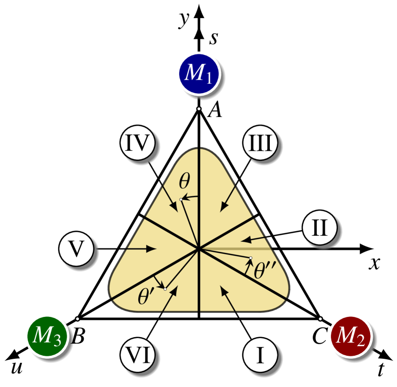
Figure 2: A hypothetical Dalitz plot for the decay $P\to M_{1}M_{2}M_{3}$, where the variables $s,t,u$ are defined in Eq.(1). The three sides of the equilateral triangle are given by $s=0$, $t=0$ and $u=0$. The three vertices $A$, $B$, $C$, correspond to $s=M^{2}$, $u=M^{2}$ and $t=M^{2}$ respectively. The three medians divide the interior of the equilateral triangle into six regions of equal area. These six sextants are denoted by $I,II,III,IV,V$ and $VI$. The three vertices $A,B,C$ of the equilateral triangle have rectangular coordinates $A=(0,2)$, $B=(-\sqrt{3},-1)$ and $C=(\sqrt{3},-1)$. This rectangular coordinate system has its origin at the center of the equilateral triangle and the $y$-axis is along the $s$-axis as shown here. The angles $\theta$, $\theta^{\prime}$ and $\theta^{\prime\prime}$ are defined in the text.The blobs with $M_{1}$, $M_{2}$ and $M_{3}$ serve as mnemonic to suggest that the exchanges $s\leftrightarrow t\leftrightarrow u$ are equivalent to the particle exchanges $M_{1}\leftrightarrow M_{2}\leftrightarrow M_{3}$ respectively. The physically allowed region is always inside the equilateral triangle as shown, schematically, by the yellow colored region.

In order to give equal weightage to $s,t$ and $u$ we shall work with a ternary plot of which $s,t,u$ form the three axes. This leads to an equilateral triangle as shown in Fig. 2. When the final particles are ultra-relativistic, the full interior of the equilateral triangle tends to get occupied. In any case the Dalitz plot under our consideration would always lie inside the equilateral triangle. The physically allowed region is schematically shown in Fig. 2 by the yellow colored region inside the equilateral triangle. The boundary of the Dalitz plot for a three-body decay process under consideration would not look symmetric under the exchanges $s\leftrightarrow t\leftrightarrow u$ due to the breaking of flavor $S\!U(3)$ symmetry on account of masses $m_{1}$, $m_{2}$ and $m_{3}$ being different. Any event inside the Dalitz plot, as illustrated in Fig. 2, can be specified by its radial distance ($r$) from the center of the equilateral triangle and the angle subtended by its position vector with any of the three axes $s,t$, or $u$. The angle subtended by the position vector with $s$-axis is denoted by $\theta$, the one with $u$-axis is denoted by $\theta^{\prime}$ and the one with $t$-axis is denoted by $\theta^{\prime\prime}$. An event described by some values of $s$, $t$ and $u$ corresponds to some values of $r$ and $\theta$ as calculable from the relations given below:

$$s =\frac{M^{2}}{3}\Big{(}1+r\,\cos\theta\Big{)},$$ (2)

$$t =\frac{M^{2}}{3}\left(1+r\,\cos\left(\frac{2\pi}{3}+\theta\right)\right),$$ (3)

$$u =\frac{M^{2}}{3}\left(1+r\,\cos\left(\frac{2\pi}{3}-\theta\right)\right).$$ (4)

One can easily change the basis from $(r,\theta)$ to either $(r,\theta^{\prime})$ or $(r,\theta^{\prime\prime})$ by noting the fact that $\theta=\theta^{\prime}+\frac{2\pi}{3}$ and $\theta=\theta^{\prime\prime}+\frac{4\pi}{3}$ (see Fig. 2).

Before we analyze the specific decay modes, we would like to point out a few simple facts about the neutral pion, which plays a pivotal role in all our decays. The neutral pion is a pure isotriplet state $\left|1,0\right\rangle_{I}\equiv\frac{1}{\sqrt{2}}\left(d\bar{d}-u\bar{u}\right)$:

$$\left|\pi^{0}\right\rangle=-\left|1,0\right\rangle_{I}.$$ (5)

But in case of $U$-spin it is a linear combination of the $U$-spin triplet state $\left|1,0\right\rangle_{U}\equiv\frac{1}{\sqrt{2}}\left(s\bar{s}-d\bar{d}\right)$ and the $U$-spin singlet but $S\!U(3)$ octet state $\left|0,0\right\rangle_{U,8}\equiv\frac{1}{\sqrt{6}}\left(d\bar{d}+s\bar{s}-2u\bar{u}\right)$:

$$\left|\pi^{0}\right\rangle=\frac{1}{2}\left|1,0\right\rangle_{U}-\frac{\sqrt{3}}{2}\left|0,0\right\rangle_{U,8}.$$ (6)

Similarly in case of $V$-spin, $\pi^{0}$ is given by a linear combination of the $V$-spin triplet state $\left|1,0\right\rangle_{V}\equiv\frac{1}{\sqrt{2}}\left(s\bar{s}-u\bar{u}\right)$ and the $V$-spin singlet but $S\!U(3)$ octet state $\left|0,0\right\rangle_{V,8}\equiv\frac{1}{\sqrt{6}}\left(u\bar{u}+s\bar{s}-2d\bar{d}\right)$:

$$\left|\pi^{0}\right\rangle=-\frac{1}{2}\left|1,0\right\rangle_{V}+\frac{\sqrt{3}}{2}\left|0,0\right\rangle_{V,8}.$$ (7)

We have put subscripts $I,U,V$ in the states to indicate that they are written in isospin, $U$-spin and $V$-spin bases respectively.

II.2 Decay Mode with final state $K^{0}\pi^{0}\pi^{+}$

We begin by considering as an example the decay mode $B^{+}\to K^{0}\pi^{0}\pi^{+}$. We will see that the application of both isospin and $U$-spin results in unique tests of the validity of both these constituent symmetries of $S\!U(3)$. The $\pi^{0}$ and $\pi^{+}$ in the final state are identical under isospin and the final state must be totally symmetric under exchange. Under $U$-spin (see Fig. 1) the $K^{0}$ and $\pi^{0}$ can be considered as identical bosons and must similarly be totally symmetric under exchange. This ensures the following exchanges in the Dalitz plot:

$$U\text{-spin exchange}\equiv K^{0}\leftrightarrow\pi^{0}\implies s\leftrightarrow t,$$

$$\text{isospin exchange}\equiv\pi^{0}\leftrightarrow\pi^{+}\implies t\leftrightarrow u.$$

Under exact $U$-spin and isospin, the final state $K^{0}\pi^{0}\pi^{+}$ has, therefore, the following two possibilities:

1. $K^{0}\pi^{0}$ would exist in either symmetrical or anti-symmetrical state w.r.t. their exchange in space, and

2. $\pi^{0}\pi^{+}$ would exist in either symmetrical or anti-symmetrical state w.r.t. their exchange in space.

The amplitude for this decay, would then be described by four independent functions defined by their symmetry and anti-symmetry properties as enunciated below:

1. $\mathcal{A}_{SS}(s,t,u)$ which is symmetric under both $s\leftrightarrow t$ and $t\leftrightarrow u$, or

2. $\mathcal{A}_{AA}(s,t,u)$ which is anti-symmetric under both $s\leftrightarrow t$ and $t\leftrightarrow u$, or

3. $\mathcal{A}_{SA}(s,t,u)$ which is symmetric under $s\leftrightarrow t$ and anti-symmetric under $t\leftrightarrow u$, or

4. $\mathcal{A}_{AS}(s,t,u)$ which is anti-symmetric under $s\leftrightarrow t$ and symmetric under $t\leftrightarrow u$.

We now analyze each of the possible amplitude functions in the most general manner. We start by $\mathcal{A}_{SS}(s,t,u)$, which is a function symmetric under both $s\leftrightarrow t$ and $t\leftrightarrow u$ to show that $\mathcal{A}_{SS}(s,t,u)$ must also be symmetric under $s\leftrightarrow u$:

$$\mathcal{A}_{SS}(s,t,u) \stackrel{{\scriptstyle s\leftrightarrow t}}{{\hbox{$\mathord{=}\mkern-7.0mu\cleaders\hbox{$\!\mathord{=}\!$}\hfill\mkern-5.0mu\mathord{=}$}}}\mathcal{A}_{SS}(t,s,u)\stackrel{{\scriptstyle t\leftrightarrow u}}{{\hbox{$\mathord{=}\mkern-7.0mu\cleaders\hbox{$\!\mathord{=}\!$}\hfill\mkern-5.0mu\mathord{=}$}}}\mathcal{A}_{SS}(u,s,t)$$

$$\stackrel{{\scriptstyle s\leftrightarrow t}}{{\hbox{$\mathord{=}\mkern-7.0mu\cleaders\hbox{$\!\mathord{=}\!$}\hfill\mkern-5.0mu\mathord{=}$}}}\mathcal{A}_{SS}(u,t,s).$$

Since, we have shown that $\mathcal{A}_{SS}(s,t,u)=\mathcal{A}_{SS}(u,t,s)$, we have demonstrated that $\mathcal{A}_{SS}(s,t,u)$ is also symmetric under $s\leftrightarrow u$. Hence, we conclude that $\mathcal{A}_{SS}(s,t,u)$ is a fully symmetric amplitude function. Let us next consider $\mathcal{A}_{AA}(s,t,u)$ which is a function anti-symmetric under both $s\leftrightarrow t$ and $t\leftrightarrow u$ to show that it is also anti-symmetric under $s\leftrightarrow u$:

$$\mathcal{A}_{AA}(s,t,u) \stackrel{{\scriptstyle s\leftrightarrow t}}{{\hbox{$\mathord{=}\mkern-7.0mu\cleaders\hbox{$\!\mathord{=}\!$}\hfill\mkern-5.0mu\mathord{=}$}}}-\mathcal{A}_{AA}(t,s,u)\stackrel{{\scriptstyle t\leftrightarrow u}}{{\hbox{$\mathord{=}\mkern-7.0mu\cleaders\hbox{$\!\mathord{=}\!$}\hfill\mkern-5.0mu\mathord{=}$}}}+\mathcal{A}_{AA}(u,s,t)$$

$$\stackrel{{\scriptstyle s\leftrightarrow t}}{{\hbox{$\mathord{=}\mkern-7.0mu\cleaders\hbox{$\!\mathord{=}\!$}\hfill\mkern-5.0mu\mathord{=}$}}}-\mathcal{A}_{AA}(u,t,s).$$

Since, $\mathcal{A}_{AA}(s,t,u)=-\mathcal{A}_{AA}(u,t,s)$ we require that $\mathcal{A}_{AA}(s,t,u)$ must also be anti-symmetric under $s\leftrightarrow u$. Hence, we conclude that $\mathcal{A}_{AA}(s,t,u)$ is a fully anti-symmetric amplitude function. Following the same arguments as above it is easy to conclude that both $\mathcal{A}_{SA}(s,t,u)$ and $\mathcal{A}_{AS}(s,t,u)$ must be identically zero. The details are as follows. The function $\mathcal{A}_{SA}(s,t,u)$ which is symmetric under $s\leftrightarrow t$ and anti-symmetric under $t\leftrightarrow u$ must satisfy

$$\mathcal{A}_{SA}(s,t,u) \stackrel{{\scriptstyle s\leftrightarrow t}}{{\hbox{$\mathord{=}\mkern-7.0mu\cleaders\hbox{$\!\mathord{=}\!$}\hfill\mkern-5.0mu\mathord{=}$}}}\mathcal{A}_{SA}(t,s,u)\stackrel{{\scriptstyle t\leftrightarrow u}}{{\hbox{$\mathord{=}\mkern-7.0mu\cleaders\hbox{$\!\mathord{=}\!$}\hfill\mkern-5.0mu\mathord{=}$}}}-\mathcal{A}_{SA}(u,s,t)$$

$$\stackrel{{\scriptstyle s\leftrightarrow t}}{{\hbox{$\mathord{=}\mkern-7.0mu\cleaders\hbox{$\!\mathord{=}\!$}\hfill\mkern-5.0mu\mathord{=}$}}}-\mathcal{A}_{SA}(u,t,s)\stackrel{{\scriptstyle t\leftrightarrow u}}{{\hbox{$\mathord{=}\mkern-7.0mu\cleaders\hbox{$\!\mathord{=}\!$}\hfill\mkern-5.0mu\mathord{=}$}}}+\mathcal{A}_{SA}(t,u,s)$$

$$\stackrel{{\scriptstyle s\leftrightarrow t}}{{\hbox{$\mathord{=}\mkern-7.0mu\cleaders\hbox{$\!\mathord{=}\!$}\hfill\mkern-5.0mu\mathord{=}$}}}+\mathcal{A}_{SA}(s,u,t)\stackrel{{\scriptstyle t\leftrightarrow u}}{{\hbox{$\mathord{=}\mkern-7.0mu\cleaders\hbox{$\!\mathord{=}\!$}\hfill\mkern-5.0mu\mathord{=}$}}}-\mathcal{A}_{SA}(s,t,u)=0.$$

Similarly, $\mathcal{A}_{AS}(s,t,u)$ being a function anti-symmetric under $s\leftrightarrow t$ and symmetric under $t\leftrightarrow u$ satisfies

$$\mathcal{A}_{AS}(s,t,u) \stackrel{{\scriptstyle s\leftrightarrow t}}{{\hbox{$\mathord{=}\mkern-7.0mu\cleaders\hbox{$\!\mathord{=}\!$}\hfill\mkern-5.0mu\mathord{=}$}}}-\mathcal{A}_{AS}(t,s,u)\stackrel{{\scriptstyle t\leftrightarrow u}}{{\hbox{$\mathord{=}\mkern-7.0mu\cleaders\hbox{$\!\mathord{=}\!$}\hfill\mkern-5.0mu\mathord{=}$}}}-\mathcal{A}_{AS}(u,s,t)$$

$$\stackrel{{\scriptstyle s\leftrightarrow t}}{{\hbox{$\mathord{=}\mkern-7.0mu\cleaders\hbox{$\!\mathord{=}\!$}\hfill\mkern-5.0mu\mathord{=}$}}}+\mathcal{A}_{AS}(u,t,s)\stackrel{{\scriptstyle t\leftrightarrow u}}{{\hbox{$\mathord{=}\mkern-7.0mu\cleaders\hbox{$\!\mathord{=}\!$}\hfill\mkern-5.0mu\mathord{=}$}}}+\mathcal{A}_{AS}(t,u,s)$$

$$\stackrel{{\scriptstyle s\leftrightarrow t}}{{\hbox{$\mathord{=}\mkern-7.0mu\cleaders\hbox{$\!\mathord{=}\!$}\hfill\mkern-5.0mu\mathord{=}$}}}-\mathcal{A}_{AS}(s,u,t)\stackrel{{\scriptstyle t\leftrightarrow u}}{{\hbox{$\mathord{=}\mkern-7.0mu\cleaders\hbox{$\!\mathord{=}\!$}\hfill\mkern-5.0mu\mathord{=}$}}}-\mathcal{A}_{AS}(s,t,u)=0.$$

We have shown that both $\mathcal{A}_{SA}(s,t,u)=0$ and $\mathcal{A}_{SA}(s,t,u)=0$, which implies that these amplitudes never contribute to the distribution of events on the Dalitz plot. Since, the function describing the distribution of events in the Dalitz plot is proportional to the amplitude mod-square, it also has only two parts, one which is fully symmetric under $s\leftrightarrow t\leftrightarrow u$, and another which is fully anti-symmetric under $s\leftrightarrow t\leftrightarrow u$.

We now examine the decay mode $B^{+}\to K^{0}\pi^{0}\pi^{+}$ in detail, by writing down the decay amplitude in terms of isospin and $U$-spin amplitudes, eventually obtaining the same conclusion as above about the distribution of events in the Dalitz plot under consideration. The $\pi^{0}\pi^{+}$ combination can exist in isospin states $\left|2,+1\right\rangle_{I}$ and $\left|1,+1\right\rangle_{I}$ (see Table 1). If isospin were an exact symmetry, the state $\left|\pi^{0}\pi^{+}\right\rangle$ would remain unchanged under $\pi^{0}\leftrightarrow\pi^{+}$ exchange. This puts the $\left|2,+1\right\rangle_{I}$ state in a space symmetric (even partial wave) state, and the $\left|1,+1\right\rangle_{I}$ state in a space anti-symmetric (odd partial wave) state. The isospin decomposition of the final state $\left|K^{0}\pi^{0}\pi^{+}\right\rangle$ is given by

$$\left|K^{0}\pi^{0}\pi^{+}\right\rangle =-\frac{1}{\sqrt{5}}\left|\frac{5}{2},+\frac{1}{2}\right\rangle_{I}^{e}+\frac{\sqrt{3}}{\sqrt{10}}\left|\frac{3}{2},+\frac{1}{2}\right\rangle_{I}^{e}$$

$$\quad+\frac{1}{\sqrt{6}}\left|\frac{3}{2},+\frac{1}{2}\right\rangle_{I}^{o}-\frac{1}{\sqrt{3}}\left|\frac{1}{2},+\frac{1}{2}\right\rangle_{I}^{o},$$ (8)

where the superscripts $e,o$ denote the even, odd nature of the state under the exchange $\pi^{0}\leftrightarrow\pi^{+}$. The sign change in the odd states above is due to the odd $\left|1,+1\right\rangle_{I}$ isospin component of the $\left|\pi^{0}\pi^{+}\right\rangle$ state switching sign under $\pi^{0}\leftrightarrow\pi^{+}$ exchange, whereas the $\left|2,+1\right\rangle_{I}$ is even under the same exchange. Since $B^{+}$ has isospin state $\left|\frac{1}{2},+\frac{1}{2}\right\rangle_{I}$, and only $\Delta I=0,1$ currents are allowed by the Hamiltonian in standard model, we would have no contributions from $\left|\frac{5}{2},+\frac{1}{2}\right\rangle_{I}$ state. The $\left|\frac{3}{2},+\frac{1}{2}\right\rangle_{I}$ state can arise from both $\left|\frac{1}{2},-\frac{1}{2}\right\rangle_{I}\otimes\left|2,+1\right\rangle_{I}$ and $\left|\frac{1}{2},-\frac{1}{2}\right\rangle_{I}\otimes\left|1,+1\right\rangle_{I}$, with the first contribution being symmetric and the later being anti-symmetric. The state $\left|\frac{1}{2},+\frac{1}{2}\right\rangle_{I}$ on the other-hand is purely anti-symmetric. Even though we shall work with the standard model Hamiltonian, our conclusions are general and are valid even when more general Hamiltonians exist.

The isospin $I=\frac{1}{2}$ initial state decays to a final state that can be decomposed into either $I=\frac{1}{2}$ or $I=\frac{3}{2}$ states via a Hamiltonian that allows $\Delta I=0$ or $\Delta I=1$ transitions. The transition with $\Delta I=1$ results in two amplitudes with $I=\frac{1}{2}$ or $I=\frac{3}{2}$ represented as $T_{\!\scriptscriptstyle{1,\frac{1}{2}}}$ and $T_{\!\scriptscriptstyle{1,\frac{3}{2}}}$ respectively, whereas $\Delta I=0$ transition results only in a single amplitude with final state $I=\frac{1}{2}$ labeled as $T_{\!\scriptscriptstyle{0,\frac{1}{2}}}$. The isospin amplitudes $T_{\!\scriptscriptstyle{1,\frac{1}{2}}}$, $T_{\!\scriptscriptstyle{1,\frac{3}{2}}}$ and $T_{\!\scriptscriptstyle{0,\frac{1}{2}}}$ are themselves defined Lipkin:1991st in terms of the Hamiltonian to be:

$$T_{\!\scriptscriptstyle{1,\frac{3}{2}}} = \sqrt{\frac{1}{3}}\left\langle\frac{3}{2},\pm\frac{1}{2}\right\lvert\mathscr{H}_{\Delta I=1}\left\rvert\frac{1}{2},\pm\frac{1}{2}\right\rangle,$$

$$T_{\!\scriptscriptstyle{1,\frac{1}{2}}} = \pm\sqrt{\frac{2}{3}}\left\langle\frac{1}{2},\pm\frac{1}{2}\right\lvert\mathscr{H}_{\Delta I=1}\left\rvert\frac{1}{2},\pm\frac{1}{2}\right\rangle,$$

$$T_{\!\scriptscriptstyle{0,\frac{1}{2}}} = \sqrt{\frac{2}{3}}\left\langle\frac{1}{2},\pm\frac{1}{2}\right\lvert\mathscr{H}_{\Delta I=0}\left\rvert\frac{1}{2},\pm\frac{1}{2}\right\rangle.$$ (9)

The amplitude for the decay $B^{+}\to K^{0}\pi^{0}\pi^{+}$ can then be written in terms of the isospin amplitudes as

$$A(B^{+}\to K^{0}\pi^{0}\pi^{+}) =\displaystyle\frac{3}{\sqrt{10}}T_{\!\scriptscriptstyle{1,\frac{3}{2}}}^{{\rm e}}\,X$$

$$\quad-\frac{1}{\sqrt{2}}\Big{(}T_{\!\scriptscriptstyle{1,\frac{3}{2}}}^{{\rm o}}+T_{\!\scriptscriptstyle{1,\frac{1}{2}}}^{{\rm o}}+T_{\!\scriptscriptstyle{0,\frac{1}{2}}}^{{\rm o}}\Big{)}\,Y\sin\theta,$$ (10)

where $X$ and $Y\sin\theta$ are introduced to take care of the spatial and kinematic contributions as is seen from the discussion above (see Eqns. (3) and (4)). In general, $X$ and $Y$ can be arbitrary functions of $r$ and $\cos\theta$. The functions $X$ and $Y$ are in general mode dependent, however, they are same for modes related by isospin symmetry. We retain the subscripts ‘${\rm e}$’ and ‘${\rm o}$’ merely to track the even or odd isospin state of the two pion in the three-body final state.

On the other hand, if $U$-spin were an exact symmetry the state $K^{0}\pi^{0}$ must remain unchanged under $K^{0}\leftrightarrow\pi^{0}$ exchange. Under $U$-spin the $K^{0}\pi^{0}$ state can exist in $\left|2,+1\right\rangle_{U}$ and $\left|1,+1\right\rangle_{U}$ (see Table 1), out of which $\left|1,+1\right\rangle_{U}$ has a contribution from the $\left|0,0\right\rangle_{U,8}$ admixture in $\pi^{0}$ which is denoted by $\left|1^{\prime},+1\right\rangle_{U}$. Both $\left|2,+1\right\rangle_{U}$ and the $\left|1,+1\right\rangle_{U}$ coming from the $\left|0,0\right\rangle_{U,8}$ contribution of $\pi^{0}$ exist in space symmetric (even partial wave) states, and that part of $\left|1,+1\right\rangle_{U}$ arising out of $\left|1,0\right\rangle_{U}$ part of $\pi^{0}$ exists in space anti-symmetric (odd partial wave) state. The $U$-spin decomposition of the final state $\left|K^{0}\pi^{0}\pi^{+}\right\rangle$ is given by

$$\left|K^{0}\pi^{0}\pi^{+}\right\rangle =-\frac{1}{2\sqrt{5}}\left|\frac{5}{2},+\frac{1}{2}\right\rangle_{U}^{e}-\frac{\sqrt{3}}{2\sqrt{10}}\left|\frac{3}{2},+\frac{1}{2}\right\rangle_{U}^{e}$$

$$\quad-\frac{1}{2\sqrt{6}}\left|\frac{3}{2},+\frac{1}{2}\right\rangle_{U}^{o}-\frac{1}{2\sqrt{3}}\left|\frac{1}{2},+\frac{1}{2}\right\rangle_{U}^{o}$$

$$\quad+\frac{1}{2}\left|\frac{3^{\prime}}{2},+\frac{1}{2}\right\rangle_{U}^{e}+\frac{1}{\sqrt{2}}\left|\frac{1^{\prime}}{2},+\frac{1}{2}\right\rangle_{U}^{e},$$ (11)

where the superscripts $e,o$ denote that the state is even, odd under the exchange $K^{0}\leftrightarrow\pi^{0}$. The origin of sign change in the odd terms above is easy to understand from the $U$-spin decomposition of the $\left|K^{0}\pi^{0}\right\rangle$ state:

$$\left|K^{0}\pi^{0}\right\rangle=\frac{1}{2\sqrt{2}}\Big{(}\left|2,+1\right\rangle_{U}+\left|1,+1\right\rangle_{U}\Big{)}-\frac{\sqrt{3}}{2}\left|1^{\prime},+1\right\rangle_{U},$$

which transforms as follows under the $K^{0}\leftrightarrow\pi^{0}$ exchange

$$\left|\pi^{0}K^{0}\right\rangle=\frac{1}{2\sqrt{2}}\Big{(}\left|2,+1\right\rangle_{U}-\left|1,+1\right\rangle_{U}\Big{)}-\frac{\sqrt{3}}{2}\left|1^{\prime},+1\right\rangle_{U}.$$

We recollect that $\left|1,+1\right\rangle_{U}$ is an odd state under $K^{0}\leftrightarrow\pi^{0}$ exchange, whereas $\left|2,+1\right\rangle_{U}$ and $\left|1^{\prime},+1\right\rangle_{U}$ are even states under the same exchange. It is easy to see that $\left|\frac{5}{2},+\frac{1}{2}\right\rangle_{U}$ and $\left|\frac{3}{2},+\frac{1}{2}\right\rangle_{U}$ states do not contribute since the parent particle $B^{+}$ is a $U$-spin singlet, and only the $\Delta U=\tfrac{1}{2}$ current contributes to the decay. This unique feature follows from the fact that the electroweak penguin does not violate $U$-spin as $d$ and $s$ quarks carry the same electric charge (see Soni:2006vi ). Hence, only the $\left|\frac{1}{2},\frac{1}{2}\right\rangle_{U}$ and $\left|\frac{1^{\prime}}{2},\frac{1}{2}\right\rangle_{U}$ can contribute to the decay amplitude and they correspond to anti-symmetric and symmetric contributions under $K^{0}\leftrightarrow\pi^{0}$ respectively. The $U$-spin amplitudes

$$U_{\!\scriptscriptstyle{\frac{1}{2},\frac{1}{2}}} = \pm\sqrt{\frac{2}{3}}\bigg{\langle}\frac{1}{2},\pm\frac{1}{2}\bigg{\lvert}\mathscr{H}_{\Delta U=\tfrac{1}{2}}\bigg{\rvert}0,0\bigg{\rangle}~{},$$

$$U^{\prime\,}_{\!\scriptscriptstyle{\frac{1}{2},\frac{1}{2}}} = \sqrt{\frac{1}{3}}\bigg{\langle}\frac{1^{\prime}}{2},\pm\frac{1}{2}\bigg{\lvert}\mathscr{H}_{\Delta U=\tfrac{1}{2}}\bigg{\rvert}0,0\bigg{\rangle}.$$ (12)

Hence, the amplitude for the decay $B^{+}\to K^{0}\pi^{0}\pi^{+}$ can then be written in terms of the $U$-spin amplitudes as

$$A(B^{+}\to K^{0}\pi^{0}\pi^{+})=\displaystyle\frac{3}{\sqrt{10}}U^{\prime\,{\rm e}}_{\!\scriptscriptstyle{\frac{1}{2},\frac{1}{2}}}\,X^{\prime}+U_{\!\scriptscriptstyle{\frac{1}{2},\frac{1}{2}}}^{{\rm o}}\,Y^{\prime}\sin\theta^{\prime},$$ (13)

where $X^{\prime}$ and $Y^{\prime}$ are functions that are, in general, arbitrary functions of $r$ and $\cos\theta^{\prime}$, and are introduced to take care of spatial and kinematic contributions to the decay amplitude. The subscripts ‘${\rm e}$’ and ‘${\rm o}$’ are again retained to merely track the even or odd $U$-spin state of $K^{0}$ and $\pi^{0}$ in the three-body final state. As argued earlier the amplitude for the decay has two parts, one fully symmetric under the exchanges $s\leftrightarrow t\leftrightarrow u$ (i.e. $\mathcal{A}_{SS}(s,t,u)$) and another fully anti-symmetric under the same exchanges (i.e. $\mathcal{A}_{AA}(s,t,u)$). Comparing Eqs. (II.2) and (13) we obtain:

$$\mathcal{A}_{SS} = \frac{3}{\sqrt{10}}T_{\!\scriptscriptstyle{1,\frac{3}{2}}}^{{\rm e}}\,X=\frac{3}{\sqrt{10}}U^{\prime\,{\rm e}}_{\!\scriptscriptstyle{\frac{1}{2},\frac{1}{2}}}\,X^{\prime}$$ (14)

$$\mathcal{A}_{AA} = -\frac{1}{\sqrt{2}}\Big{(}T_{\!\scriptscriptstyle{1,\frac{3}{2}}}^{{\rm o}}+T_{\!\scriptscriptstyle{1,\frac{1}{2}}}^{{\rm o}}+T_{\!\scriptscriptstyle{0,\frac{1}{2}}}^{{\rm o}}\Big{)}\,Y\sin\theta$$ (15)

$$= U_{\!\scriptscriptstyle{\frac{1}{2},\frac{1}{2}}}^{{\rm o}}\,Y^{\prime}\sin\theta^{\prime}.$$

The exchange $s\leftrightarrow t\leftrightarrow u$ being equivalent to $\theta\leftrightarrow\theta^{\prime}\leftrightarrow\theta^{\prime\prime}$, implies that the fully anti-symmetric amplitude $\mathcal{A}_{AA}(s,t,u)$ must be proportional to $\sin 3\theta$ because $\sin 3\theta=\sin 3\theta^{\prime}=\sin 3\theta^{\prime\prime}$ as $\theta=\theta^{\prime}+\frac{2\pi}{3}=\theta^{\prime\prime}+\frac{4\pi}{3}$. From elementary trigonometry we know that $\sin 3\theta=\sin\theta\,\left(4\cos^{2}\theta-1\right)$. This implies that the factor $\left(4\cos^{2}\theta-1\right)$ is an even function of $\cos\theta$ and is a part of both $Y$ and $Y^{\prime}$ in Eq. (15), i.e. $Y=y\left(4\cos^{2}\theta-1\right)$ and $Y^{\prime}=y^{\prime}\left(4\cos^{2}\theta^{\prime}-1\right)$ for some $y$ and $y^{\prime}$ such that

$$\mathcal{A}_{AA} =-\frac{1}{\sqrt{2}}\Big{(}T_{\!\scriptscriptstyle{1,\frac{3}{2}}}^{{\rm o}}+T_{\!\scriptscriptstyle{1,\frac{1}{2}}}^{{\rm o}}+T_{\!\scriptscriptstyle{0,\frac{1}{2}}}^{{\rm o}}\Big{)}\,y\sin 3\theta$$

$$=U_{\!\scriptscriptstyle{\frac{1}{2},\frac{1}{2}}}^{{\rm o}}\,y^{\prime}\sin 3\theta^{\prime}.$$ (16)

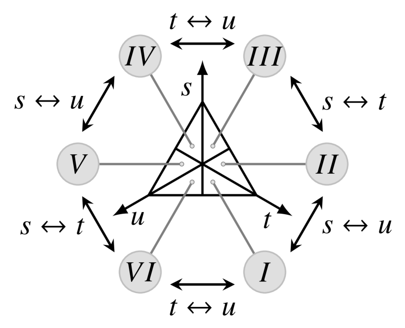
Figure 3: Exchanges that take us from one sextant to another in the Dalitz plot. It must be noted that the following exchanges are also equivalent: $s\leftrightarrow t\leftrightarrow u\equiv\theta\leftrightarrow\theta^{\prime}\leftrightarrow\theta^{\prime\prime}$ as well as $t\leftrightarrow u\equiv\theta\leftrightarrow-\theta$, $s\leftrightarrow t\equiv\theta^{\prime}\leftrightarrow-\theta^{\prime}$ and $u\leftrightarrow s\equiv\theta^{\prime\prime}\leftrightarrow-\theta^{\prime\prime}$.

The Dalitz plot can be divided into six sextants by means of the $s$, $t$ and $u$ axes which go along the medians of an equilateral triangle as shown in Figs. 2 and 3. Since the Dalitz plot distribution function is proportional to the amplitude mod-square, it would also have a part which is fully symmetric under $s\leftrightarrow t\leftrightarrow u$ (denoted by $f_{SS}(s,t,u)$) and another part which is fully anti-symmetric under the same exchanges (denoted by $f_{AA}(s,t,u)$):

$$f_{SS}(s,t,u) \propto\left|\mathcal{A}_{SS}(s,t,u)\right|^{2}+\left|\mathcal{A}_{AA}(s,t,u)\right|^{2},$$ (17)

$$f_{AA}(s,t,u) \propto 2\,\text{Re}\Big{(}\mathcal{A}_{SS}(s,t,u)\cdot\mathcal{A}_{AA}^{*}(s,t,u)\Big{)}.$$ (18)

Let us denote the function describing distribution of events in any sextant, say the $i$th one, of the Dalitz plot by $f_{i}(r,\theta)$, where the coordinates $(r,\theta)$ lie in the sextant $i$ and we could have as well used the other equivalent choices $\theta^{\prime}$ or $\theta^{\prime\prime}$ instead of $\theta$, the choice of which is subject to the underlying symmetry being considered (see Fig. 3). Henceforth we shall drop $(r,\theta)$ from the distribution functions, except when necessary, as we implicitly assume the $r$ and $\theta$ dependence in them. The distribution function must have only two parts as said above, the fully symmetric and the fully anti-symmetric parts. Let us assume that in sextant $I$ the Dalitz plot distribution is given by the function

$$f_{I}=f_{SS}(s,t,u)+f_{AA}(s,t,u).$$ (19)

It is then trivial to see that the Dalitz plot distributions in the even numbered sextants should be identical to one another, and the odd numbered sextants would also be identically populated, because

$$f_{I}=f_{III}=f_{V} =f_{SS}(s,t,u)+f_{AA}(s,t,u),$$ (20)

$$f_{II}=f_{IV}=f_{VI} =f_{SS}(s,t,u)-f_{AA}(s,t,u).$$ (21)

This is the signature of exact $S\!U(3)$ flavor symmetry in the Dalitz plots under our consideration. Any deviation from this conclusion would constitute an observable evidence for violation of the $S\!U(3)$ flavor symmetry.

Until now the exchange properties of $K^{0}\leftrightarrow\pi^{0}$ under $U$-spin and $\pi^{0}\leftrightarrow\pi^{+}$ under isospin have been used to obtain the even and odd amplitudes contributing to $B^{+}\to K^{0}\pi^{0}\pi^{+}$. Since $K^{0}$ and $\pi^{+}$ belong to different multiplets of $V$-spin, in order to consider the symmetry properties under $K^{0}\leftrightarrow\pi^{+}$ one needs to define the $G$-parity analogue of $V$-spin, denoted by $G_{\!V}$ and defined in the Appendix A. Since charge conjugation is a good symmetry in strong interaction, $G_{\!V}$ is as good as $V$-spin itself. The state $\left|K^{0}\pi^{+}\right\rangle$ is composed of states which are even and odd under $G_{\!V}$-parity:

$$\left|K^{0}\pi^{+}\right\rangle=\frac{1}{2}\left(\left|K^{0}\pi^{+}\right\rangle_{\rm e}+\left|K^{0}\pi^{+}\right\rangle_{\rm o}\right),$$

where

$$\left|K^{0}\pi^{+}\right\rangle_{\rm e} =\left|K^{0}\pi^{+}\right\rangle-\left|\pi^{+}K^{0}\right\rangle,$$

$$\left|K^{0}\pi^{+}\right\rangle_{\rm o} =\left|K^{0}\pi^{+}\right\rangle+\left|\pi^{+}K^{0}\right\rangle,$$

and

$$G_{\!V}\left|K^{0}\pi^{+}\right\rangle_{\rm e} =+\left|K^{0}\pi^{+}\right\rangle_{\rm e},$$

$$G_{\!V}\left|K^{0}\pi^{+}\right\rangle_{\rm o} =-\left|K^{0}\pi^{+}\right\rangle_{\rm o}.$$

We have already proven that the amplitudes for the decay $B^{+}\to K^{0}\pi^{0}\pi^{+}$ has two parts one even and the other odd under the exchange of any two particles in the final state. Hence, $\mathcal{A}_{SS}$ is odd under $G_{\!V}$ and $\mathcal{A}_{AA}$ is even under $G_{\!V}$. Since the two $G_{\!V}$-parity amplitudes do not interfere the two amplitudes $\mathcal{A}_{SS}$ and $\mathcal{A}_{AA}$ do not interfere in the Dalitz plot distribution resulting in $f_{AA}$ being zero (Eq. (18)). Therefore if $G_{\!V}$ is a good symmetry of nature it is interesting to conclude that the Dalitz plot is completely symmetric under $s\leftrightarrow t\leftrightarrow u$. This implies that

$$f_{I}=f_{II}=f_{III}=f_{IV}=f_{V}=f_{VI}\equiv f_{SS}(s,t,u).$$ (22)

This expression holds only if isospin, $U$-spin and $V$-spin are all exact symmetries. However, if $G_{\!V}$ is broken the Dalitz plot distribution will still follow Eqs. (20) and (21) when isospin and $U$-spin are exact symmetries. In the case when $G_{\!V}$ is exact, the exchange properties of the distribution functions $f_{I}$ to $f_{VI}$ imply that if, (a) $U$-spin is an exact symmetry, then $f_{II}=f_{III}$, $f_{I}=f_{IV}$ and $f_{V}=f_{VI}$ irrespective of the validity of isospin symmetry, (b) isospin is an exact symmetry, then $f_{II}=f_{V}$, $f_{I}=f_{VI}$ and $f_{III}=f_{IV}$ irrespective of the validity of $U$-spin symmetry. However, when both $G_{\!V}$ and either isospin or $U$-spin is broken, then the Eqs. (20) and (21) are no longer valid. In such a case, we have the following possibilities:

• Test for isospin symmetry: By isospin symmetry, the sextants $I,II,III$ get mapped to the sextants $VI,V,IV$ respectively. We note that when isospin is not broken, then

  $$f_{I}+f_{VI} =f_{III}+f_{IV}=f_{V}+f_{II}=2f_{SS}(s,t,u),$$ (23)

  $$f_{I}-f_{VI} =f_{III}-f_{IV}=f_{V}-f_{II}=2f_{AA}(s,t,u).$$ (24)

  However, when isospin is broken, the values of $f_{SS}$ and $f_{AA}$ extracted from sextants $I$ and $VI$ need not be same with those extracted from either $II$ and $V$ or $III$ and $IV$. For further clarification of this statement, we introduce two quantities $\Sigma^{i}_{j}$ and $\Delta^{i}_{j}$ defined as

  $$\Sigma^{i}_{j}(r,\theta) =f_{i}+f_{j},$$ (25)

  $$\Delta^{i}_{j}(r,\theta) =f_{i}-f_{j},$$ (26)

  where $i$ and $j$ are two sextants and $i\neq j$. For conciseness of expressions, we shall also drop the explicit $(r,\theta)$ dependence of $\Sigma^{i}_{j}$ and $\Delta^{i}_{j}$. In terms of these quantities, the signature of isospin breaking can be succinctly summarized by the inequalities

  $$\Sigma^{I}_{VI}\neq\Sigma^{III}_{IV}\neq\Sigma^{V}_{II},$$ (27)

  $$\Delta^{I}_{VI}\neq\Delta^{III}_{IV}\neq\Delta^{V}_{II}.$$ (28)

  An asymmetry can now the constructed to measure the isospin breaking as follows:

  $$\mathbb{A}_{\text{Isospin}} =\left|\frac{\Sigma^{I}_{VI}-\Sigma^{III}_{IV}}{\Sigma^{I}_{VI}+\Sigma^{III}_{IV}}\right|+\left|\frac{\Sigma^{III}_{IV}-\Sigma^{V}_{II}}{\Sigma^{III}_{IV}+\Sigma^{V}_{II}}\right|+\left|\frac{\Sigma^{V}_{II}-\Sigma^{I}_{VI}}{\Sigma^{V}_{II}+\Sigma^{I}_{VI}}\right|$$

  $$\quad+\left|\frac{\Delta^{I}_{VI}-\Delta^{III}_{IV}}{\Delta^{I}_{VI}+\Delta^{III}_{IV}}\right|+\left|\frac{\Delta^{III}_{IV}-\Delta^{V}_{II}}{\Delta^{III}_{IV}+\Delta^{V}_{II}}\right|+\left|\frac{\Delta^{V}_{II}-\Delta^{I}_{VI}}{\Delta^{V}_{II}+\Delta^{I}_{VI}}\right|.$$ (29)

• Test for $U$-spin symmetry: By $U$spin symmetry, the sextants $VI,I,II$ get mapped to the sextants $V,IV,III$ respectively. We note that when $U$-spin is not broken, then

  $$\Sigma^{I}_{IV}=\Sigma^{III}_{II}=\Sigma^{V}_{VI}=2f_{SS}(s,t,u),$$ (30)

  $$\Delta^{I}_{IV}=\Delta^{III}_{II}=\Delta^{V}_{VI}=2f_{AA}(s,t,u).$$ (31)

  Here it is profitable to consider the $\Sigma$’s and $\Delta$’s being functions of $(r,\theta^{\prime})$ as we are considering $s\leftrightarrow t$ exchange which is equivalent to $\theta^{\prime}\leftrightarrow-\theta^{\prime}$. When $U$-spin is broken

  $$\Sigma^{I}_{IV}\neq\Sigma^{III}_{II}\neq\Sigma^{V}_{VI},$$ (32)

  $$\Delta^{I}_{IV}\neq\Delta^{III}_{II}\neq\Delta^{V}_{VI}.$$ (33)

  The asymmetry for $U$-spin breaking is, therefore, given by

  $$\mathbb{A}_{U\text{-spin}} =\left|\frac{\Sigma^{I}_{IV}-\Sigma^{III}_{II}}{\Sigma^{I}_{IV}+\Sigma^{III}_{II}}\right|+\left|\frac{\Sigma^{III}_{II}-\Sigma^{V}_{VI}}{\Sigma^{III}_{II}+\Sigma^{V}_{VI}}\right|+\left|\frac{\Sigma^{V}_{VI}-\Sigma^{I}_{IV}}{\Sigma^{V}_{VI}+\Sigma^{I}_{IV}}\right|$$

  $$\quad+\left|\frac{\Delta^{I}_{IV}-\Delta^{III}_{II}}{\Delta^{I}_{IV}+\Delta^{III}_{II}}\right|+\left|\frac{\Delta^{III}_{II}-\Delta^{V}_{VI}}{\Delta^{III}_{II}+\Delta^{V}_{VI}}\right|+\left|\frac{\Delta^{V}_{VI}-\Delta^{I}_{IV}}{\Delta^{V}_{VI}+\Delta^{I}_{IV}}\right|.$$ (34)

• Test for $V$-spin symmetry: As said before, $G_{\!V}$-parity is as badly broken as the $V$-spin because charge conjugation is a good symmetry. When $V$-spin symmetry is broken, then $G_{\!V}$ is also broken, and the distribution of events in the Dalitz plot sextants would follow Eqs. (20) and (21). In addition to that, when $V$-spin is broken, $K^{0}$ and $\pi^{+}$ need not be even under exchange. This leads to

  $$\Sigma_{IV}^{V}\neq\Sigma_{VI}^{III}\neq\Sigma_{II}^{I},$$ (35)

  $$\Delta_{IV}^{V}\neq\Delta_{VI}^{III}\neq\Delta_{II}^{I}.$$ (36)

  The asymmetry for $V$-spin breaking is, therefore, given by

  $$\mathbb{A}_{V\text{-spin}} =\left|\frac{\Sigma^{V}_{IV}-\Sigma^{I}_{II}}{\Sigma^{V}_{IV}+\Sigma^{I}_{II}}\right|+\left|\frac{\Sigma^{I}_{II}-\Sigma^{III}_{VI}}{\Sigma^{I}_{II}+\Sigma^{III}_{VI}}\right|+\left|\frac{\Sigma^{III}_{VI}-\Sigma^{V}_{IV}}{\Sigma^{III}_{VI}+\Sigma^{V}_{IV}}\right|$$

  $$\quad+\left|\frac{\Delta^{V}_{IV}-\Delta^{I}_{II}}{\Delta^{V}_{IV}+\Delta^{I}_{II}}\right|+\left|\frac{\Delta^{I}_{II}-\Delta^{III}_{VI}}{\Delta^{I}_{II}+\Delta^{III}_{VI}}\right|+\left|\frac{\Delta^{III}_{VI}-\Delta^{V}_{IV}}{\Delta^{III}_{VI}+\Delta^{V}_{IV}}\right|.$$ (37)

Hence, the extent of the breaking of isospin, $U$-spin and $V$-spin can easily be measured from the Dalitz plot distribution. The asymmetries measuring isospin, $U$-spin and $V$-spin are functions of $r$ and $3\theta\equiv 3\theta^{\prime}\equiv 3\theta^{\prime\prime}$ (see the discussion leading to Eq. (II.2)). These asymmetries are, thus, valid in the full Dalitz plot, including the resonant contributions and can be measured in different regions of the Dalitz plot. In particular these asymmetries can be measured both along resonances and in the non-resonant regions. A quantitative estimate of the variation of these asymmetries obtained experimentally would provide valuable understanding of $S\!U(3)$ breaking effects. It would also be interesting to find regions of the Dalitz plots where $S\!U(3)$ is a good symmetry. The procedure discussed above can also be applied to other decay modes with the same final state. In particular one can study the Dalitz plot distribution for the decay $D^{+}_{s}\to K^{0}\pi^{0}\pi^{+}$ in a similar manner. The amplitudes for this mode are tabulated in Table. 2.

$B^{+}\to K^{0}\pi^{0}\pi^{+}$
Isospin (initial state $\left|\frac{1}{2},+\frac{1}{2}\right\rangle$)				$U$-spin (initial state $\left|0,0\right\rangle$)
transition	final state	symmetry	Amplitude	transition	final state	symmetry	Amplitude
$\Delta I=1$	$\left|\frac{3}{2},+\frac{1}{2}\right\rangle$	mixed	$\frac{3}{\sqrt{10}}T_{\!1,\frac{3}{2}}^{e}X+\frac{1}{\sqrt{2}}T_{\!1,\frac{3}{2}}^{o}Y\sin\theta$	$\Delta U=\frac{1}{2}$	$\left|\frac{1}{2},+\frac{1}{2}\right\rangle$	odd	$-\frac{1}{2\sqrt{2}}U_{\!\frac{1}{2},\frac{3}{2}}^{o}Y^{\prime}\sin\theta^{\prime}$
$\Delta I=1$	$\left|\frac{1}{2},+\frac{1}{2}\right\rangle$	odd	$-\frac{1}{\sqrt{2}}T_{\!1,\frac{1}{2}}^{o}Y\sin\theta$	$\Delta U=\frac{1}{2}^{\prime}$	$\left|\frac{1}{2},+\frac{1}{2}^{\prime}\right\rangle$	even	$\frac{\sqrt{3}}{\sqrt{2}}U_{\!\frac{1}{2},\frac{1}{2}^{\prime}}^{\prime e}X^{\prime}$
$\Delta I=0$	$\left|\frac{1}{2},+\frac{1}{2}\right\rangle$	odd	$-\frac{1}{\sqrt{2}}T_{\!0,\frac{1}{2}}^{o}Y\sin\theta$
$D^{+}_{s}\to K^{0}\pi^{0}\pi^{+}$
Isospin (initial state $\left|0,0\right\rangle$)				$U$-spin (initial state $\left|\frac{1}{2},+\frac{1}{2}\right\rangle$)
transition	final state	symmetry	Amplitude	transition	final state	symmetry	Amplitude
$\Delta I=\frac{3}{2}$	$\left|\frac{3}{2},+\frac{1}{2}\right\rangle$	mixed	$\frac{\sqrt{3}}{\sqrt{10}}T_{\!\frac{3}{2},\frac{3}{2}}^{e}X+\frac{1}{\sqrt{6}}T_{\!\frac{3}{2},\frac{3}{2}}^{o}Y\sin\theta$	$\Delta U=1$	$\left|\frac{3}{2},+\frac{1}{2}\right\rangle$	mixed	$-\frac{3}{2\sqrt{10}}U_{1,\frac{3}{2}}^{e}X^{\prime}-\frac{1}{2\sqrt{2}}U_{\!1,\frac{3}{2}}^{o}Y^{\prime}\sin\theta^{\prime}$
$\Delta I=\frac{1}{2}$	$\left|\frac{1}{2},+\frac{1}{2}\right\rangle$	odd	$-\frac{1}{\sqrt{2}}T_{\!\frac{1}{2},\frac{1}{2}}^{o}Y\sin\theta$	$\Delta U=1$	$\left|\frac{3}{2}^{\prime},+\frac{1}{2}\right\rangle$	even	$\frac{\sqrt{3}}{2}U_{\!1,\frac{3}{2}^{\prime}}^{\prime e}X^{\prime}$
				$\Delta U=1$	$\left|\frac{1}{2},+\frac{1}{2}\right\rangle$	odd	$-\frac{1}{2\sqrt{2}}U_{1,\frac{1}{2}}^{o}Y^{\prime}\sin\theta^{\prime}$
				$\Delta U=1$	$\left|\frac{1}{2}^{\prime},+\frac{1}{2}\right\rangle$	even	$\frac{\sqrt{3}}{2}U_{1,\frac{1}{2}^{\prime}}^{\prime e}X^{\prime}$
				$\Delta U=0$	$\left|\frac{1}{2},+\frac{1}{2}\right\rangle$	odd	$-\frac{1}{2\sqrt{2}}U_{0,\frac{1}{2}}^{o}Y^{\prime}\sin\theta^{\prime}$
				$\Delta U=0$	$\left|\frac{1}{2}^{\prime},+\frac{1}{2}\right\rangle$	even	$\frac{\sqrt{3}}{2}U_{0,\frac{1}{2}^{\prime}}^{\prime e}X^{\prime}$

Table 2: Comparison of decays of $B^{+}$ and $D^{+}_{s}$ to the final state $K^{0}\pi^{0}\pi^{+}$.

II.3 Decay Mode with final state $K^{+}\pi^{0}\pi^{-}$

$B^{0}_{d}\to K^{+}\pi^{0}\pi^{-}$
Isospin (initial state $\left|\frac{1}{2},-\frac{1}{2}\right\rangle$)				$V$-spin (initial state $\left|0,0\right\rangle$)
transition	final state	symmetry	Amplitude	transition	final state	symmetry	Amplitude
$\Delta I=1$	$\left|\frac{3}{2},-\frac{1}{2}\right\rangle$	mixed	$\frac{3}{\sqrt{10}}T_{\!1,\frac{3}{2}}^{e}X+\frac{1}{\sqrt{2}}T_{\!1,\frac{3}{2}}^{o}Y\sin\theta$	$\Delta V=\frac{3}{2}$	$\left|\frac{3}{2},+\frac{1}{2}\right\rangle$	mixed	$\frac{\sqrt{3}}{2\sqrt{10}}V_{\!\frac{3}{2},\frac{3}{2}}^{e}X^{\prime\prime}+\frac{1}{2\sqrt{6}}V_{\!\frac{3}{2},\frac{3}{2}}^{o}Y^{\prime\prime}\sin\theta^{\prime\prime}$
$\Delta I=1$	$\left|\frac{1}{2},-\frac{1}{2}\right\rangle$	odd	$-\frac{1}{\sqrt{2}}T_{\!1,\frac{1}{2}}^{o}Y\sin\theta$	$\Delta V=\frac{3}{2}$	$\left|\frac{3}{2}^{\prime},+\frac{1}{2}\right\rangle$	even	$-\frac{1}{2}V_{\!\frac{3}{2},\frac{3}{2}^{\prime}}^{\prime e}X^{\prime\prime}$
$\Delta I=0$	$\left|\frac{1}{2},-\frac{1}{2}\right\rangle$	odd	$\frac{1}{\sqrt{2}}T_{\!0,\frac{1}{2}}^{o}Y\sin\theta$	$\Delta V=\frac{1}{2}$	$\left|\frac{1}{2},+\frac{1}{2}\right\rangle$	odd	$\frac{1}{2\sqrt{2}}V_{\!\frac{1}{2},\frac{1}{2}}^{o}Y^{\prime\prime}\sin\theta^{\prime\prime}$
				$\Delta V=\frac{1}{2}$	$\left|\frac{1}{2}^{\prime},+\frac{1}{2}\right\rangle$	even	$-\frac{\sqrt{3}}{\sqrt{2}}V_{\!\frac{1}{2},\frac{1}{2}^{\prime}}^{\prime e}X^{\prime\prime}$
$\kern 1.79993pt\bar{\kern-1.79993ptB}{}^{0}_{s}\to K^{+}\pi^{0}\pi^{-}$
Isospin (initial state $\left|0,0\right\rangle$)				$V$-spin (initial state $\left|\frac{1}{2},+\frac{1}{2}\right\rangle$)
transition	final state	symmetry	Amplitude	transition	final state	symmetry	Amplitude
$\Delta I=\frac{3}{2}$	$\left|\frac{3}{2},-\frac{1}{2}\right\rangle$	mixed	$\frac{\sqrt{3}}{\sqrt{10}}T_{\!\frac{3}{2},\frac{3}{2}}^{e}X+\frac{1}{\sqrt{6}}T_{\!\frac{3}{2},\frac{3}{2}}^{o}Y\sin\theta$	$\Delta V=1$	$\left|\frac{3}{2},+\frac{1}{2}\right\rangle$	mixed	$\frac{3}{2\sqrt{10}}V_{\!1,\frac{3}{2}}^{e}X^{\prime\prime}+\frac{1}{2\sqrt{2}}V_{\!1,\frac{3}{2}}^{o}Y^{\prime\prime}\sin\theta^{\prime\prime}$
$\Delta I=\frac{1}{2}$	$\left|\frac{1}{2},-\frac{1}{2}\right\rangle$	odd	$-\frac{1}{\sqrt{2}}T_{\!\frac{1}{2},\frac{1}{2}}^{o}Y\sin\theta$	$\Delta V=1$	$\left|\frac{3}{2}^{\prime},+\frac{1}{2}\right\rangle$	even	$-\frac{\sqrt{3}}{2}V_{\!1,\frac{3}{2}^{\prime}}^{\prime e}X^{\prime\prime}$
				$\Delta V=1$	$\left|\frac{1}{2},+\frac{1}{2}\right\rangle$	odd	$\frac{1}{2\sqrt{2}}V_{\!1,\frac{1}{2}}^{o}Y^{\prime\prime}\sin\theta^{\prime\prime}$
				$\Delta V=1$	$\left|\frac{1}{2}^{\prime},+\frac{1}{2}\right\rangle$	even	$-\frac{\sqrt{3}}{2}V_{\!1,\frac{1}{2}^{\prime}}^{e}X^{\prime\prime}$
				$\Delta V=0$	$\left|\frac{1}{2},+\frac{1}{2}\right\rangle$	odd	$\frac{1}{2\sqrt{2}}V_{\!0,\frac{1}{2}}^{o}Y^{\prime\prime}\sin\theta^{\prime\prime}$
				$\Delta V=0$	$\left|\frac{1}{2}^{\prime},+\frac{1}{2}\right\rangle$	even	$-\frac{\sqrt{3}}{2}V_{\!0,\frac{1}{2}^{\prime}}^{\prime e}X^{\prime\prime}$

Table 3: Comparison of decays of $B^{0}_{d}$ and $\kern 1.79993pt\bar{\kern-1.79993ptB}{}^{0}_{s}$ to the final state $K^{+}\pi^{0}\pi^{-}$.

Let us now consider the decay $B^{0}_{d}\text{ or }\kern 1.79993pt\bar{\kern-1.79993ptB}{}^{0}_{s}\to K^{+}\pi^{0}\pi^{-}$ in which isospin symmetry allows the exchange of $\pi^{0}$ and $\pi^{-}$, and $V$-spin symmetry allows exchange of $K^{+}$ and $\pi^{0}$. This leads to the following exchanges in the Dalitz plot:

$$V\text{-spin}\equiv K^{+}\leftrightarrow\pi^{0}\implies s\leftrightarrow t,$$

$$\text{Isospin}\equiv\pi^{0}\leftrightarrow\pi^{-}\implies t\leftrightarrow u.$$

Under exact isospin and $V$-spin, the final state $K^{+}\pi^{0}\pi^{-}$ has, the following two possibilities:

1. $K^{+}\pi^{0}$ would exist in either symmetrical or anti-symmetrical state w.r.t. their exchange in space, and

2. $\pi^{0}\pi^{-}$ would exist in either symmetrical or anti-symmetrical state w.r.t. their exchange in space.

Following the steps as enunciated in subsection II.2, the amplitude for the decay can be shown to have two components, one which is fully symmetric under exchange of any pair of final particles, and the other fully anti-symmetric under the same exchange.

The final state can be expanded in terms of isospin and $V$-spin states as follows:

• Isospin

  $$\left|K^{+}\pi^{0}\pi^{-}\right\rangle =\frac{1}{\sqrt{5}}\left|\frac{5}{2},-\frac{1}{2}\right\rangle_{I}^{e}+\sqrt{\frac{3}{10}}\left|\frac{3}{2},-\frac{1}{2}\right\rangle_{I}^{e}$$

  $$\quad+\frac{1}{\sqrt{6}}\left|\frac{3}{2},-\frac{1}{2}\right\rangle_{I}^{o}+\frac{1}{\sqrt{3}}\left|\frac{1}{2},-\frac{1}{2}\right\rangle_{I}^{o},$$ (38)

  where the superscripts $e,o$ denote even, odd behavior of the state under the exchange $\pi^{0}\leftrightarrow\pi^{-}$.

• $V$-spin

  $$\left|K^{+}\pi^{0}\pi^{-}\right\rangle =\frac{1}{2\sqrt{5}}\left|\frac{5}{2},+\frac{1}{2}\right\rangle_{V}^{e}+\frac{\sqrt{3}}{2\sqrt{10}}\left|\frac{3}{2},+\frac{1}{2}\right\rangle_{V}^{e}$$

  $$\quad+\frac{1}{2\sqrt{6}}\left|\frac{3}{2},+\frac{1}{2}\right\rangle_{V}^{o}+\frac{1}{2\sqrt{3}}\left|\frac{1}{2},+\frac{1}{2}\right\rangle_{V}^{o}$$

  $$\quad-\frac{1}{2}\left|\frac{3^{\prime}}{2},+\frac{1}{2}\right\rangle_{V}^{e}-\frac{1}{\sqrt{2}}\left|\frac{1^{\prime}}{2},+\frac{1}{2}\right\rangle_{V}^{e},$$

  where the superscripts $e,o$ denote even, odd behavior of the state under the exchange $K^{+}\leftrightarrow\pi^{0}$.

The sign changes as can be noticed in the above states arise from exchange of particles in the two particle states given below (as also noted in Table 1):

• Isospin:

  $$\left|\pi^{0}\pi^{-}\right\rangle =\frac{1}{\sqrt{2}}\Big{(}\left|2,-1\right\rangle_{I}+\left|1,-1\right\rangle_{I}\Big{)},$$ (39)

  $$\left|\pi^{-}\pi^{0}\right\rangle =\frac{1}{\sqrt{2}}\Big{(}\left|2,-1\right\rangle_{I}-\left|1,-1\right\rangle_{I}\Big{)}.$$ (40)

• $V$-spin:

  $$\left|K^{+}\pi^{0}\right\rangle =-\frac{1}{2\sqrt{2}}\Big{(}\left|2,+1\right\rangle_{V}+\left|1,+1\right\rangle_{V}\Big{)}+\frac{\sqrt{3}}{2}\left|1^{\prime},+1\right\rangle_{V},$$ (41)

  $$\left|\pi^{0}K^{+}\right\rangle =-\frac{1}{2\sqrt{2}}\Big{(}\left|2,+1\right\rangle_{V}-\left|1,+1\right\rangle_{V}\Big{)}+\frac{\sqrt{3}}{2}\left|1^{\prime},+1\right\rangle_{V}.$$ (42)

It would be clear from the expressions above that if isospin were an exact symmetry, the $\left|2,-1\right\rangle_{I}$ and $\left|1,-1\right\rangle_{I}$ states of $\left|\pi^{-}\pi^{0}\right\rangle$ would exist in even and odd partial wave states respectively, as was the case in subsection II.2 also. On the other hand, if $V$-spin were an exact symmetry the state $\left|K^{+}\pi^{0}\right\rangle$ must remain unchanged under $K^{+}\leftrightarrow\pi^{0}$ exchange. Under $V$-spin the $\left|K^{+}\pi^{0}\right\rangle$ state can exist in $\left|2,+1\right\rangle_{V}$ and $\left|1,+1\right\rangle_{V}$, out of which $\left|1,+1\right\rangle_{V}$ has a contribution from the $\left|0,0\right\rangle_{V,8}$ admixture in $\pi^{0}$, denoted above by $\left|1^{\prime},+1\right\rangle_{V}$. Both state $\left|2,+1\right\rangle_{V}$ and the state $\left|1^{\prime},+1\right\rangle_{V}$ exist in space symmetric (even partial wave) states, and that part of $\left|1,+1\right\rangle_{V}$ arising out of $\left|1,0\right\rangle_{V}$ part of $\pi^{0}$ exists in space anti-symmetric (odd partial wave) state.

If we consider the initial state to be $B^{0}_{d}$ which is isospin $\left|\frac{1}{2},+\frac{1}{2}\right\rangle_{I}$ state but $V$-spin singlet $\left|0,0\right\rangle_{V}$ state, the standard model Hamiltonian allows only $\Delta I=0,1$ and $\Delta V=\frac{1}{2},\frac{3}{2}$ transitions. Therefore, in addition to the isospin amplitudes of Eq. II.2, we can define the following $V$-spin amplitudes:

$$V_{\frac{3}{2},\frac{3}{2}} =\bigg{\langle}\frac{3}{2},\pm\frac{1}{2}\bigg{\lvert}\mathscr{H}_{\Delta V=\frac{3}{2}}\bigg{\rvert}0,0\bigg{\rangle}~{},$$ (43)

$$V^{\prime}_{\frac{3}{2},\frac{3}{2}} =\bigg{\langle}\frac{3}{2}^{\prime},\pm\frac{1}{2}\bigg{\lvert}\mathscr{H}_{\Delta V=\frac{3}{2}}\bigg{\rvert}0,0\bigg{\rangle}~{},$$ (44)

$$V_{\!\scriptscriptstyle{\frac{1}{2},\frac{1}{2}}} =\pm\sqrt{\frac{2}{3}}\bigg{\langle}\frac{1}{2},\pm\frac{1}{2}\bigg{\lvert}\mathscr{H}_{\Delta V=\tfrac{1}{2}}\bigg{\rvert}0,0\bigg{\rangle}~{},$$ (45)

$$V^{\prime\,}_{\!\scriptscriptstyle{\frac{1}{2},\frac{1}{2}}} =\sqrt{\frac{1}{3}}\bigg{\langle}\frac{1^{\prime}}{2},\pm\frac{1}{2}\bigg{\lvert}\mathscr{H}_{\Delta V=\tfrac{1}{2}}\bigg{\rvert}0,0\bigg{\rangle}.$$ (46)

The amplitude for the process $B^{0}_{d}\to K^{+}\pi^{0}\pi^{-}$ can, therefore, be written as

$$A(B^{0}_{d}\to K^{+}\pi^{0}\pi^{-}) =-\frac{3}{\sqrt{10}}T_{\!\scriptscriptstyle{1,\frac{3}{2}}}^{e}X+\frac{1}{\sqrt{2}}\left(-T_{\!\scriptscriptstyle{1,\frac{1}{2}}}^{o}+T_{\!\scriptscriptstyle{0,\frac{1}{2}}}^{o}\right)Y\sin\theta,$$ (47)

$$A(B^{0}_{d}\to K^{+}\pi^{0}\pi^{-}) =\sqrt{\frac{3}{2}}\left(\frac{1}{\sqrt{20}}V_{\frac{3}{2},\frac{3}{2}}^{e}-\frac{1}{\sqrt{6}}V_{\frac{3}{2},\frac{3}{2}^{\prime}}^{\prime e}-V_{\frac{1}{2},\frac{1}{2}^{\prime}}^{\prime e}\right)X^{\prime\prime}$$

$$\quad+\frac{1}{2\sqrt{2}}\left(\frac{1}{\sqrt{3}}V_{\frac{3}{2},\frac{3}{2}}^{o}+V_{\frac{1}{2},\frac{1}{2}}^{o}\right)Y^{\prime\prime}\sin\theta^{\prime\prime},$$ (48)

where $X^{\prime\prime}$ and $Y^{\prime\prime}$ are functions that are, in general, arbitrary functions of $r$ and $\cos\theta^{\prime\prime}$, and are introduced to take care of spatial and kinematic contributions to the decay amplitude. As argued before, the part of the amplitude even under isospin must also be even under $V$-spin and the part odd under isospin must again be odd under $V$-spin:

$$\mathcal{A}_{SS} =\frac{3}{\sqrt{10}}T_{\!\scriptscriptstyle{1,\frac{3}{2}}}^{{\rm e}}\,X$$

$$=\sqrt{\frac{3}{2}}\left(\frac{1}{\sqrt{20}}V_{\frac{3}{2},\frac{3}{2}}^{e}-\frac{1}{\sqrt{6}}V_{\frac{3}{2},\frac{3}{2}^{\prime}}^{\prime e}-V_{\frac{1}{2},\frac{1}{2}^{\prime}}^{\prime e}\right)X^{\prime\prime},$$ (49)

$$\mathcal{A}_{AA} =\frac{1}{\sqrt{2}}(-T_{\!\scriptscriptstyle{1,\frac{1}{2}}}^{{\rm o}}+T_{\!\scriptscriptstyle{0,\frac{1}{2}}}^{{\rm o}})\,Y\sin\theta$$

$$=\frac{1}{2\sqrt{2}}\left(\frac{1}{\sqrt{3}}V_{\frac{3}{2},\frac{3}{2}}^{o}+V_{\frac{1}{2},\frac{1}{2}}^{o}\right)Y^{\prime\prime}\sin\theta^{\prime\prime}.$$ (50)

We can conclude that the Dalitz plot distribution in the even numbered sextants would be identical to one another, and those of odd numbered sextants would also be similar. Any deviation from this would constitute a signature of simultaneous violations of isospin and $V$-spin.

Since $K^{+}$ and $\pi^{-}$ belong to different multiplets of $U$-spin, in order to consider the symmetry properties under $K^{+}\leftrightarrow\pi^{-}$ one needs to define the $G$-parity analogue of $U$-spin, denoted by $G_{\!U}$ and defined in the Appendix A. Since charge conjugation is a good symmetry in strong interaction, $G_{\!U}$ is as good as $U$-spin itself. The state $\left|K^{+}\pi^{-}\right\rangle$ is composed of states which are even and odd under $G_{\!U}$-parity:

$$\left|K^{+}\pi^{-}\right\rangle=\frac{1}{2}\left(\left|K^{+}\pi^{-}\right\rangle_{\rm e}+\left|K^{+}\pi^{-}\right\rangle_{\rm o}\right),$$

where

$$\left|K^{+}\pi^{-}\right\rangle_{e} =\left|K^{+}\pi^{-}\right\rangle-\left|\pi^{-}K^{+}\right\rangle,$$

$$\left|K^{+}\pi^{-}\right\rangle_{o} =\left|K^{+}\pi^{-}\right\rangle+\left|\pi^{-}K^{+}\right\rangle,$$

and

$$G_{\!U}\left|K^{+}\pi^{-}\right\rangle_{e} =\left|K^{+}\pi^{-}\right\rangle_{e},$$

$$G_{\!U}\left|K^{+}\pi^{-}\right\rangle_{o} =-\left|K^{+}\pi^{-}\right\rangle_{o}.$$

We have already proven that the amplitudes for the decay $B^{0}_{d}\to K^{+}\pi^{0}\pi^{-}$ has two parts one even and the other odd under the exchange of any two particles in the final state. Hence, $\mathcal{A}_{SS}$ is odd under $G_{\!U}$ and $\mathcal{A}_{AA}$ is even under $G_{\!U}$. Since the two $G_{\!U}$-parity amplitudes do not interfere the two amplitudes $\mathcal{A}_{SS}$ and $\mathcal{A}_{AA}$ do not interfere in the Dalitz plot distribution resulting in $f_{AA}$ being zero (Eq. (18)). Therefore if $G_{\!U}$ is a good symmetry of nature it is interesting to conclude that the Dalitz plot is completely symmetric under $s\leftrightarrow t\leftrightarrow u$. The Dalitz plot asymmetries which would be a measure of the extent of breaking of the $S\!U(3)$ flavor symmetry are, therefore, given by

$$\mathbb{A}_{\text{Isospin}} =\left|\frac{\Sigma^{I}_{VI}-\Sigma^{III}_{IV}}{\Sigma^{I}_{VI}+\Sigma^{III}_{IV}}\right|+\left|\frac{\Sigma^{III}_{IV}-\Sigma^{V}_{II}}{\Sigma^{III}_{IV}+\Sigma^{V}_{II}}\right|+\left|\frac{\Sigma^{V}_{II}-\Sigma^{I}_{VI}}{\Sigma^{V}_{II}+\Sigma^{I}_{VI}}\right|$$

$$\quad+\left|\frac{\Delta^{I}_{VI}-\Delta^{III}_{IV}}{\Delta^{I}_{VI}+\Delta^{III}_{IV}}\right|+\left|\frac{\Delta^{III}_{IV}-\Delta^{V}_{II}}{\Delta^{III}_{IV}+\Delta^{V}_{II}}\right|+\left|\frac{\Delta^{V}_{II}-\Delta^{I}_{VI}}{\Delta^{V}_{II}+\Delta^{I}_{VI}}\right|,$$ (51)

$$\mathbb{A}_{U\text{-spin}} =\left|\frac{\Sigma^{V}_{IV}-\Sigma^{I}_{II}}{\Sigma^{V}_{IV}+\Sigma^{I}_{II}}\right|+\left|\frac{\Sigma^{I}_{II}-\Sigma^{III}_{VI}}{\Sigma^{I}_{II}+\Sigma^{III}_{VI}}\right|+\left|\frac{\Sigma^{III}_{VI}-\Sigma^{V}_{IV}}{\Sigma^{III}_{VI}+\Sigma^{V}_{IV}}\right|$$

$$\quad+\left|\frac{\Delta^{V}_{IV}-\Delta^{I}_{II}}{\Delta^{V}_{IV}+\Delta^{I}_{II}}\right|+\left|\frac{\Delta^{I}_{II}-\Delta^{III}_{VI}}{\Delta^{I}_{II}+\Delta^{III}_{VI}}\right|+\left|\frac{\Delta^{III}_{VI}-\Delta^{V}_{IV}}{\Delta^{III}_{VI}+\Delta^{V}_{IV}}\right|,$$ (52)

$$\mathbb{A}_{V\text{-spin}} =\left|\frac{\Sigma^{I}_{IV}-\Sigma^{III}_{II}}{\Sigma^{I}_{IV}+\Sigma^{III}_{II}}\right|+\left|\frac{\Sigma^{III}_{II}-\Sigma^{V}_{VI}}{\Sigma^{III}_{II}+\Sigma^{V}_{VI}}\right|+\left|\frac{\Sigma^{V}_{VI}-\Sigma^{I}_{IV}}{\Sigma^{V}_{VI}+\Sigma^{I}_{IV}}\right|$$

$$\quad+\left|\frac{\Delta^{I}_{IV}-\Delta^{III}_{II}}{\Delta^{I}_{IV}+\Delta^{III}_{II}}\right|+\left|\frac{\Delta^{III}_{II}-\Delta^{V}_{VI}}{\Delta^{III}_{II}+\Delta^{V}_{VI}}\right|+\left|\frac{\Delta^{V}_{VI}-\Delta^{I}_{IV}}{\Delta^{V}_{VI}+\Delta^{I}_{IV}}\right|,$$ (53)

where the $\Sigma$’s and $\Delta$’s are as defined in Eqs. (25) and (26) respectively. It must again be noted that these asymmetries are in general functions of $r$ and $\theta$ (or $\theta^{\prime}$ or $\theta^{\prime\prime}$), and are defined throughout the Dalitz plot region, including resonant regions. It would again be interesting to look for patterns in the variations of these asymmetries inside the Dalitz plot. Observation of these asymmetries would quantify the extent of breaking of $S\!U(3)$ flavor symmetry in the concerned decay mode. One can also look for such asymmetries in the Dalitz plot for $\kern 1.79993pt\bar{\kern-1.79993ptB}{}^{0}_{s}\to K^{+}\pi^{0}\pi^{-}$. The amplitudes for this process are given in Table 3.

II.4 Decay Mode with final state $K^{+}\pi^{0}\kern 1.99997pt\bar{\kern-1.99997ptK}{}^{0}$

$B^{+}\to K^{+}\pi^{0}\kern 1.99997pt\bar{\kern-1.99997ptK}{}^{0}$
$U$-spin (initial state $\left|0,0\right\rangle$)				$V$-spin (initial state $\left|\frac{1}{2},+\frac{1}{2}\right\rangle$)
transition	final state	symmetry	Amplitude	transition	final state	symmetry	Amplitude
$\Delta U=\frac{1}{2}$	$\left|\frac{1}{2},-\frac{1}{2}\right\rangle$	odd	$\frac{1}{2\sqrt{2}}U_{\!\frac{1}{2},\frac{1}{2}}^{o}Y^{\prime}\sin\theta^{\prime}$	$\Delta V=1$	$\left|\frac{3}{2},+\frac{1}{2}\right\rangle$	mixed	$-\frac{3}{2\sqrt{10}}V_{\!1,\frac{3}{2}}^{e}X^{\prime\prime}-\frac{1}{2\sqrt{2}}V_{\!1,\frac{3}{2}}^{o}Y^{\prime\prime}\sin\theta^{\prime\prime}$
$\Delta U=\frac{1}{2}$	$\left|\frac{1}{2}^{\prime},-\frac{1}{2}\right\rangle$	even	$\frac{\sqrt{3}}{\sqrt{2}}U_{\!\frac{1}{2},\frac{1}{2}^{\prime}}^{\prime e}X^{\prime}$	$\Delta V=1$	$\left|\frac{3}{2}^{\prime},+\frac{1}{2}\right\rangle$	even	$\frac{\sqrt{3}}{2}V_{\!1,\frac{3}{2}^{\prime}}^{\prime e}X^{\prime\prime}$
$\Delta U=\frac{3}{2}$	$\left|\frac{3}{2},-\frac{1}{2}\right\rangle$	mixed	$\frac{\sqrt{3}}{2\sqrt{10}}U_{\!\frac{3}{2},\frac{3}{2}}^{e}X^{\prime}-\frac{1}{2\sqrt{6}}U_{\!\frac{3}{2},\frac{3}{2}}^{o}Y^{\prime}\sin\theta^{\prime}$	$\Delta V=1$	$\left|\frac{1}{2},+\frac{1}{2}\right\rangle$	odd	$-\frac{1}{2\sqrt{2}}V_{\!1,\frac{1}{2}}^{o}Y^{\prime\prime}\sin\theta^{\prime\prime}$
$\Delta U=\frac{3}{2}$	$\left|\frac{3}{2}^{\prime},-\frac{1}{2}\right\rangle$	even	$\frac{1}{2}U_{\!\frac{1}{2},\frac{1}{2}^{\prime}}^{\prime e}X^{\prime}$	$\Delta V=1$	$\left|\frac{1}{2}^{\prime},+\frac{1}{2}\right\rangle$	even	$\frac{\sqrt{3}}{2}V_{\!1,\frac{1}{2}^{\prime}}^{\prime e}X^{\prime\prime}$
				$\Delta V=0$	$\left|\frac{1}{2},+\frac{1}{2}\right\rangle$	odd	$-\frac{1}{2\sqrt{2}}V_{0,\frac{1}{2}}^{o}Y^{\prime\prime}\sin\theta^{\prime\prime}$
				$\Delta V=0$	$\left|\frac{1}{2}^{\prime},+\frac{1}{2}\right\rangle$	even	$\frac{\sqrt{3}}{2}V_{0,\frac{1}{2}}^{\prime e}X^{\prime\prime}$
$D^{+}\to K^{+}\pi^{0}\kern 1.99997pt\bar{\kern-1.99997ptK}{}^{0}$
$U$-spin (initial state $-\left|\frac{1}{2},-\frac{1}{2}\right\rangle$)				$V$-spin (initial state $\left|0,0\right\rangle$)
transition	final state	symmetry	Amplitude	transition	final state	symmetry	Amplitude
$\Delta U=1$	$\left|\frac{3}{2},-\frac{1}{2}\right\rangle$	mixed	$-\frac{3}{2\sqrt{10}}U_{\!1,\frac{3}{2}}^{e}X^{\prime}-\frac{1}{2\sqrt{2}}U_{\!1,\frac{3}{2}}^{o}Y^{\prime}\sin\theta^{\prime}$	$\Delta V=\frac{3}{2}$	$\left|\frac{3}{2},+\frac{1}{2}\right\rangle$	mixed	$-\frac{\sqrt{3}}{2\sqrt{10}}V_{\!\frac{3}{2},\frac{3}{2}}^{e}X^{\prime\prime}-\frac{1}{2\sqrt{6}}V_{\!\frac{3}{2},\frac{3}{2}}^{o}Y^{\prime\prime}\sin\theta^{\prime\prime}$
$\Delta U=1$	$\left|\frac{3}{2}^{\prime},-\frac{1}{2}\right\rangle$	even	$\frac{\sqrt{3}}{2}U_{\!1,\frac{3}{2}^{\prime}}^{\prime e}X^{\prime}$	$\Delta V=\frac{3}{2}$	$\left|\frac{3}{2}^{\prime},+\frac{1}{2}\right\rangle$	even	$\frac{1}{2}V_{\!\frac{3}{2},\frac{3}{2}^{\prime}}^{\prime e}X^{\prime\prime}$
$\Delta U=1$	$\left|\frac{1}{2},-\frac{1}{2}\right\rangle$	odd	$\frac{1}{2\sqrt{2}}U_{\!1,\frac{1}{2}}^{o}Y^{\prime}\sin\theta^{\prime}$	$\Delta V=\frac{1}{2}$	$\left|\frac{1}{2},+\frac{1}{2}\right\rangle$	odd	$-\frac{1}{2}V_{\!\frac{1}{2},\frac{1}{2}}^{o}Y^{\prime\prime}\sin\theta^{\prime\prime}$
$\Delta U=1$	$\left|\frac{1}{2}^{\prime},-\frac{1}{2}\right\rangle$	even	$-\frac{\sqrt{3}}{2}U_{1,\frac{1}{2}^{\prime}}^{\prime e}X^{\prime}$	$\Delta V=\frac{1}{2}$	$\left|\frac{1}{2}^{\prime},+\frac{1}{2}\right\rangle$	even	$\frac{\sqrt{3}}{\sqrt{2}}V_{\!\frac{1}{2},\frac{1}{2}^{\prime}}^{\prime e}X^{\prime\prime}$
$\Delta U=0$	$\left|\frac{1}{2},-\frac{1}{2}\right\rangle$	odd	$-\frac{1}{2\sqrt{2}}U_{\!0,\frac{1}{2}}^{o}Y^{\prime}\sin\theta^{\prime}$
$\Delta U=0$	$\left|\frac{1}{2}^{\prime},-\frac{1}{2}\right\rangle$	even	$\frac{\sqrt{3}}{2}U_{0,\frac{1}{2}^{\prime}}^{\prime e}X^{\prime}$

Table 4: Comparison of amplitudes for the decays of $B^{+}$ and $D^{+}$ to the final state $K^{+}\pi^{0}\kern 1.99997pt\bar{\kern-1.99997ptK}{}^{0}$.

For study of simultaneous violations of both $U$-spin and $V$-spin, we look at decays such as $B^{+}\text{ or }D^{+}\to K^{+}\pi^{0}\kern 1.99997pt\bar{\kern-1.99997ptK}{}^{0}$ and their conjugate modes. In this state, $K^{+}$ and $\pi^{0}$ are exchangeable under $V$-spin and $\pi^{0},\kern 1.99997pt\bar{\kern-1.99997ptK}{}^{0}$ are exchangeable under $U$-spin. Under $V$-spin, the $K^{+}\pi^{0}$ state can exist in $\left|2,+1\right\rangle_{V}$ and $\left|1,+1\right\rangle_{V}$, out of which the state $\left|1,+1\right\rangle_{V}$ has a contribution from the $\left|0,0\right\rangle_{V,8}$ admixture in $\pi^{0}$. Thus assuming $V$-spin to be an exact symmetry would put the state $\left|2,+1\right\rangle_{V}$ and that part of $\left|1,+1\right\rangle_{V}$ state coming from $\left|0,0\right\rangle_{V,8}$ contribution of $\pi^{0}$ in space symmetric (even partial wave) state. The remaining part of $\left|1,+1\right\rangle_{V}$ state would be in space anti-symmetric (odd partial wave) state. Similarly, the $\pi^{0}\kern 1.99997pt\bar{\kern-1.99997ptK}{}^{0}$ state would exist in $\left|2,-1\right\rangle_{U}$ and $\left|1,-1\right\rangle_{U}$, out of which the state $\left|1,-1\right\rangle_{U}$ has a contribution from the $\left|0,0\right\rangle_{U,8}$ admixture in $\pi^{0}$. Thus, if $U$-spin were assumed to be an exact symmetry, the states $\left|2,-1\right\rangle_{U}$ and the $\left|1,-1\right\rangle_{U}$ state coming from $\left|0,0\right\rangle_{U,8}$ part of $\pi^{0}$ would exist in space symmetric (even partial wave) states, and the other part of $\left|1,-1\right\rangle_{U}$ would exist in space anti-symmetric (odd partial wave) state.

Therefore, under exact $U$-spin and $V$-spin, the final state $K^{+}\pi^{0}\kern 1.99997pt\bar{\kern-1.99997ptK}{}^{0}$ has, the following two possibilities:

1. $K^{+}\pi^{0}$ would exist in either symmetrical or anti-symmetrical state w.r.t. their exchange in space, and

2. $\pi^{0}\kern 1.99997pt\bar{\kern-1.99997ptK}{}^{0}$ would exist in either symmetrical or anti-symmetrical state w.r.t. their exchange in space.

Again, following the steps as enunciated in subsection II.2 we can conclude that the Dalitz plot distribution in the even numbered sextants would be identical to one another, and those of odd numbered sextants would also be similar, as given in Eqs. (20) and (21). Any deviation from this would constitute a signature of simultaneous violations of $U$-spin and $V$-spin. We can once again reaffirm the same logic as given in subsections II.2 and II.3, by invoking the $G_{\!I}$-parity operator (see Appendix A) to connect $K^{+}$ and $\kern 1.99997pt\bar{\kern-1.99997ptK}{}^{0}$ belonging to two different isospin doublets. This would lead to a fully symmetric Dalitz plot which would be broken when $G_{\!I}$ is broken. The amplitudes for the two decay modes under consideration are given in Table 4. The Dalitz plot asymmetries that can be useful in this case are given by

$$\mathbb{A}_{\text{Isospin}} =\left|\frac{\Sigma^{V}_{IV}-\Sigma^{I}_{II}}{\Sigma^{V}_{IV}+\Sigma^{I}_{II}}\right|+\left|\frac{\Sigma^{I}_{II}-\Sigma^{III}_{VI}}{\Sigma^{I}_{II}+\Sigma^{III}_{VI}}\right|+\left|\frac{\Sigma^{III}_{VI}-\Sigma^{V}_{IV}}{\Sigma^{III}_{VI}+\Sigma^{V}_{IV}}\right|$$

$$\quad+\left|\frac{\Delta^{V}_{IV}-\Delta^{I}_{II}}{\Delta^{V}_{IV}+\Delta^{I}_{II}}\right|+\left|\frac{\Delta^{I}_{II}-\Delta^{III}_{VI}}{\Delta^{I}_{II}+\Delta^{III}_{VI}}\right|+\left|\frac{\Delta^{III}_{VI}-\Delta^{V}_{IV}}{\Delta^{III}_{VI}+\Delta^{V}_{IV}}\right|,$$ (54)

$$\mathbb{A}_{U\text{-spin}} =\left|\frac{\Sigma^{I}_{VI}-\Sigma^{III}_{IV}}{\Sigma^{I}_{VI}+\Sigma^{III}_{IV}}\right|+\left|\frac{\Sigma^{III}_{IV}-\Sigma^{V}_{II}}{\Sigma^{III}_{IV}+\Sigma^{V}_{II}}\right|+\left|\frac{\Sigma^{V}_{II}-\Sigma^{I}_{VI}}{\Sigma^{V}_{II}+\Sigma^{I}_{VI}}\right|$$

$$\quad+\left|\frac{\Delta^{I}_{VI}-\Delta^{III}_{IV}}{\Delta^{I}_{VI}+\Delta^{III}_{IV}}\right|+\left|\frac{\Delta^{III}_{IV}-\Delta^{V}_{II}}{\Delta^{III}_{IV}+\Delta^{V}_{II}}\right|+\left|\frac{\Delta^{V}_{II}-\Delta^{I}_{VI}}{\Delta^{V}_{II}+\Delta^{I}_{VI}}\right|,$$ (55)

$$\mathbb{A}_{V\text{-spin}} =\left|\frac{\Sigma^{I}_{IV}-\Sigma^{III}_{II}}{\Sigma^{I}_{IV}+\Sigma^{III}_{II}}\right|+\left|\frac{\Sigma^{III}_{II}-\Sigma^{V}_{VI}}{\Sigma^{III}_{II}+\Sigma^{V}_{VI}}\right|+\left|\frac{\Sigma^{V}_{VI}-\Sigma^{I}_{IV}}{\Sigma^{V}_{VI}+\Sigma^{I}_{IV}}\right|$$

$$\quad+\left|\frac{\Delta^{I}_{IV}-\Delta^{III}_{II}}{\Delta^{I}_{IV}+\Delta^{III}_{II}}\right|+\left|\frac{\Delta^{III}_{II}-\Delta^{V}_{VI}}{\Delta^{III}_{II}+\Delta^{V}_{VI}}\right|+\left|\frac{\Delta^{V}_{VI}-\Delta^{I}_{IV}}{\Delta^{V}_{VI}+\Delta^{I}_{IV}}\right|.$$ (56)

Once again the asymmetries being, in general, functions of $r$ and $\theta$ (or $\theta^{\prime}$ or $\theta^{\prime\prime}$) it would be quite interesting to look for their variation across the Dalitz plot. These would be the visible signatures of the breaking of $S\!U(3)$ flavor symmetry.

II.5 Decay Mode with final state $\pi^{+}\pi^{0}\kern 1.99997pt\bar{\kern-1.99997ptK}{}^{0}$

Finally, we consider a mode where each pair of particles in the final states can be directly related by one of the three $S\!U(2)$ symmetries, namely isospin, $U$-spin and $V$-spin. Here we do not need $G_{\!I}$, $G_{\!V}$ or $G_{\!U}$ to relate the final states. We consider as an example decays with final state $\pi^{+}\pi^{0}\kern 1.99997pt\bar{\kern-1.99997ptK}{}^{0}$ such as $D^{+}\to\pi^{+}\pi^{0}\kern 1.99997pt\bar{\kern-1.99997ptK}{}^{0}$ and the conjugate mode. In the final state considered here, isospin exchange implies $\pi^{0}\leftrightarrow\pi^{+}$, $U$-spin exchange implies $\pi^{0}\leftrightarrow\kern 1.99997pt\bar{\kern-1.99997ptK}{}^{0}$ and $V$-spin exchange implies $\pi^{+}\leftrightarrow\kern 1.99997pt\bar{\kern-1.99997ptK}{}^{0}$. The $S\!U(2)$ decompositions of all the pairs of particles under their respective $S\!U(2)$ symmetries have already been considered in subsections II.2, II.3, II.4. Once again, the steps elaborated in subsection II.2 are applicable to this case also. The amplitudes for this decay mode can be easily read off from Table 5. However, in this mode the even and odd contributions to the decay amplitude can interfere as they are not eigenstates of $G_{\!V}$, resulting in even and odd numbered sextants to have distinctly different density of events as depicted in Eqs. (20) and (21). Note that the Dalitz plot distributions for the even (odd) numbered sextants of the Dalitz plot would still be identical if isospin and $U$-spin are exact symmetries. The breakdown of isospin, $U$-spin and $V$-spin could be quantitatively measured using the following asymmetries:

$$\mathbb{A}_{\text{Isospin}} =\left|\frac{\Sigma^{I}_{IV}-\Sigma^{III}_{II}}{\Sigma^{I}_{IV}+\Sigma^{III}_{II}}\right|+\left|\frac{\Sigma^{III}_{II}-\Sigma^{V}_{VI}}{\Sigma^{III}_{II}+\Sigma^{V}_{VI}}\right|+\left|\frac{\Sigma^{V}_{VI}-\Sigma^{I}_{IV}}{\Sigma^{V}_{VI}+\Sigma^{I}_{IV}}\right|$$

$$\quad+\left|\frac{\Delta^{I}_{IV}-\Delta^{III}_{II}}{\Delta^{I}_{IV}+\Delta^{III}_{II}}\right|+\left|\frac{\Delta^{III}_{II}-\Delta^{V}_{VI}}{\Delta^{III}_{II}+\Delta^{V}_{VI}}\right|+\left|\frac{\Delta^{V}_{VI}-\Delta^{I}_{IV}}{\Delta^{V}_{VI}+\Delta^{I}_{IV}}\right|,$$ (57)

$$\mathbb{A}_{U\text{-spin}} =\left|\frac{\Sigma^{I}_{VI}-\Sigma^{III}_{IV}}{\Sigma^{I}_{VI}+\Sigma^{III}_{IV}}\right|+\left|\frac{\Sigma^{III}_{IV}-\Sigma^{V}_{II}}{\Sigma^{III}_{IV}+\Sigma^{V}_{II}}\right|+\left|\frac{\Sigma^{V}_{II}-\Sigma^{I}_{VI}}{\Sigma^{V}_{II}+\Sigma^{I}_{VI}}\right|$$

$$\quad+\left|\frac{\Delta^{I}_{VI}-\Delta^{III}_{IV}}{\Delta^{I}_{VI}+\Delta^{III}_{IV}}\right|+\left|\frac{\Delta^{III}_{IV}-\Delta^{V}_{II}}{\Delta^{III}_{IV}+\Delta^{V}_{II}}\right|+\left|\frac{\Delta^{V}_{II}-\Delta^{I}_{VI}}{\Delta^{V}_{II}+\Delta^{I}_{VI}}\right|,$$ (58)

$$\mathbb{A}_{V\text{-spin}} =\left|\frac{\Sigma^{V}_{IV}-\Sigma^{I}_{II}}{\Sigma^{V}_{IV}+\Sigma^{I}_{II}}\right|+\left|\frac{\Sigma^{I}_{II}-\Sigma^{III}_{VI}}{\Sigma^{I}_{II}+\Sigma^{III}_{VI}}\right|+\left|\frac{\Sigma^{III}_{VI}-\Sigma^{V}_{IV}}{\Sigma^{III}_{VI}+\Sigma^{V}_{IV}}\right|$$

$$\quad+\left|\frac{\Delta^{V}_{IV}-\Delta^{I}_{II}}{\Delta^{V}_{IV}+\Delta^{I}_{II}}\right|+\left|\frac{\Delta^{I}_{II}-\Delta^{III}_{VI}}{\Delta^{I}_{II}+\Delta^{III}_{VI}}\right|+\left|\frac{\Delta^{III}_{VI}-\Delta^{V}_{IV}}{\Delta^{III}_{VI}+\Delta^{V}_{IV}}\right|.$$ (59)

Once again these asymmetries being, in general, functions of $r$ and $\theta$ (or $\theta^{\prime}$ or $\theta^{\prime\prime}$) it would be very interesting to look for their variation across the Dalitz plot. These would constitute the visible signatures of the breaking of $S\!U(3)$ flavor symmetry.

$D^{+}\to\pi^{+}\pi^{0}\kern 1.99997pt\bar{\kern-1.99997ptK}{}^{0}$
Isospin (initial state $\left|\frac{1}{2},+\frac{1}{2}\right\rangle$)				$U$-spin (initial state $-\left|\frac{1}{2},-\frac{1}{2}\right\rangle$)
transition	final state	symmetry	Amplitude	transition	final state	symmetry	Amplitude
$\Delta I=1$	$\left|\frac{3}{2},+\frac{3}{2}\right\rangle$	mixed	$\frac{\sqrt{3}}{\sqrt{10}}T_{\!1,\frac{3}{2}}^{e}X+\frac{\sqrt{3}}{\sqrt{2}}T_{\!1,\frac{3}{2}}^{o}Y\sin\theta$	$\Delta U=1$	$\left|\frac{3}{2},-\frac{3}{2}\right\rangle$	mixed	$\frac{\sqrt{3}}{2\sqrt{5}}U_{\!1,\frac{3}{2}}^{e}X^{\prime}-\frac{\sqrt{3}}{2}U_{\!1,\frac{3}{2}}^{o}Y^{\prime}\sin\theta^{\prime}$
					$\left|\frac{3}{2}^{\prime},-\frac{3}{2}\right\rangle$	even	$\frac{3}{2}U_{\!1,\frac{3}{2}^{\prime}}^{\prime e}X^{\prime}$

Table 5: Amplitudes for the decay $D^{+}\to\pi^{+}\pi^{0}\kern 1.99997pt\bar{\kern-1.99997ptK}{}^{0}$. The $V$-spin amplitudes can be written in a similar manner. For brevity we have not written them explicitly.

III Conclusion

In this paper we have elucidated a new model independent method to look for the breaking of the $S\!U(3)$ flavor symmetry in many three-body decay modes, namely $B^{+}\text{ or }D^{+}_{s}\to K^{0}\pi^{0}\pi^{+}$, $B^{0}_{d}\text{ or }\kern 1.79993pt\bar{\kern-1.79993ptB}{}^{0}_{s}\to K^{+}\pi^{0}\pi^{-}$, $B^{+}\text{ or }D^{+}\to K^{+}\pi^{0}\kern 1.99997pt\bar{\kern-1.99997ptK}{}^{0}$ and $D^{+}\to\pi^{+}\pi^{0}\kern 1.99997pt\bar{\kern-1.99997ptK}{}^{0}$. The novelty in choosing these decay modes is that pairs of the final state do belong to at least two different $S\!U(2)$ triplets, and hence under the assumption of exact $S\!U(3)$ flavor symmetry, the amplitude for the process has two parts: one fully symmetric and another fully anti-symmetric under the exchanges $s\leftrightarrow t\leftrightarrow u$. This gives rise to a characteristic pattern in the Dalitz plot distribution: the alternate sextants must have identical distribution of events. Any deviation from this behavior would constitute an evidence for the breaking of $S\!U(3)$ flavor symmetry, which indeed is broken in nature. We have provided mode specific Dalitz plot asymmetries which can be used to quantify the extent of $S\!U(3)$ symmetry breaking in each of the decay modes under our consideration. These asymmetries are defined in the full region of the Dalitz plot and can be measured both along resonances and in the non-resonant regions. A quantitative estimate of the variation of these asymmetries obtained experimentally would provide a valuable understanding of $S\!U(3)$ breaking effects. It would also be interesting to find regions of the Dalitz plots where $S\!U(3)$ is a good symmetry. A better understanding and measured estimate of $S\!U(3)$ breaking would help in reliably estimating hadronic uncertainties and hence result in effectively using it to measure weak phases and search for new physics effects beyond the standard model.

Appendix A $G$-parity and final states

The $G$-parity operator $G_{\!I}$ (or $G_{\!U}$ or $G_{\!V}$) is defined as a rotation through $\pi$ radian ($180^{\circ}$) around the second axis of isospin (or $U$-spin or $V$-spin) space, followed by charge conjugation ($\mathcal{C}$): $G_{\!I}=\mathcal{C}e^{i\pi I_{2}}=\mathcal{C}e^{i\pi\tau_{2}/2},$ where $I_{2}$ is the second generator of $S\!U(2)$ isospin (or $U$-spin or $V$-spin) group, and $\tau_{2}$ is the second Pauli matrix. $G$-parity as defined here transforms the various $S\!U(2)$ multiplets as follows:

$$G_{\!I}\begin{pmatrix}\pi^{+}\\ \pi^{0}\\ \pi^{-}\end{pmatrix}=-\begin{pmatrix}\pi^{+}\\ \pi^{0}\\ \pi^{-}\end{pmatrix}, G_{\!I}\begin{pmatrix}K^{+}\\ K^{0}\end{pmatrix}=\begin{pmatrix}\kern 1.99997pt\bar{\kern-1.99997ptK}{}^{0}\\ -K^{-}\end{pmatrix}, G_{\!I}\begin{pmatrix}\kern 1.99997pt\bar{\kern-1.99997ptK}{}^{0}\\ -K^{-}\end{pmatrix}=-\begin{pmatrix}K^{+}\\ K^{0}\end{pmatrix},$$

$$G_{\!U}\begin{pmatrix}K^{0}\\ \pi^{0}\\ \kern 1.99997pt\bar{\kern-1.99997ptK}{}^{0}\end{pmatrix}=-\begin{pmatrix}K^{0}\\ \pi^{0}\\ \kern 1.99997pt\bar{\kern-1.99997ptK}{}^{0}\end{pmatrix}, G_{\!U}\begin{pmatrix}K^{+}\\ \pi^{+}\end{pmatrix}=\begin{pmatrix}\pi^{-}\\ -K^{-}\end{pmatrix}, G_{\!U}\begin{pmatrix}\pi^{-}\\ -K^{-}\end{pmatrix}=-\begin{pmatrix}K^{+}\\ \pi^{+}\end{pmatrix},$$

$$G_{\!V}\begin{pmatrix}K^{+}\\ \pi^{0}\\ K^{-}\end{pmatrix}=-\begin{pmatrix}K^{+}\\ \pi^{0}\\ K^{-}\end{pmatrix}, G_{\!V}\begin{pmatrix}\pi^{+}\\ \kern 1.99997pt\bar{\kern-1.99997ptK}{}^{0}\end{pmatrix}=\begin{pmatrix}K^{0}\\ -\pi^{-}\end{pmatrix}, G_{\!V}\begin{pmatrix}K^{0}\\ -\pi^{-}\end{pmatrix}=-\begin{pmatrix}\pi^{+}\\ \kern 1.99997pt\bar{\kern-1.99997ptK}{}^{0}\end{pmatrix},$$

References

(1) M. Gell-Mann, California Institute of Technology
Synchrotron Laboratory Report No. CTSL–20, 1961 (unpublished).
(2)
M. Gell-Mann,
Phys. Rev. 125, 1067 (1962).
(3)
Y. Ne’eman,
Nucl. Phys. 26, 222 (1961).
(4)
S. Okubo,
Prog. Theor. Phys. 27, 949 (1962).
(5)
S. Okubo and C. Ryan,
Nuovo Cim. 34, 776 (1964).
(6)
R. L. Kingsley, S. B. Treiman, F. Wilczek and A. Zee,
Phys. Rev. D 11, 1919 (1975).
(7)
M. B. Voloshin, V. I. Zakharov and L. B. Okun,
JETP Lett. 21, 183 (1975)
[Pisma Zh. Eksp. Teor. Fiz. 21, 403 (1975)].
(8)
L. L. Wang and F. Wilczek,
Phys. Rev. Lett. 43, 816 (1979).
(9)
C. Quigg,
Z. Phys. C 4, 55 (1980).
(10)
D. Zeppenfeld,
Z. Phys. C 8, 77 (1981).
(11)
L. L. Chau and H. Y. Cheng,
Phys. Rev. Lett. 56, 1655 (1986).
(12)
L. L. Chau and H. Y. Cheng,
Phys. Rev. D 36, 137 (1987).
(13)
M. J. Savage and M. B. Wise,
Phys. Rev. D 39, 3346 (1989)
[Erratum-ibid. D 40, 3127 (1989)].
(14)
L. L. Chau, H. Y. Cheng, W. K. Sze, H. Yao and B. Tseng,
Phys. Rev. D 43, 2176 (1991)
[Erratum-ibid. D 58, 019902 (1998)].
(15)
M. J. Savage,
Phys. Lett. B 257, 414 (1991).
(16)
H. J. Lipkin, Y. Nir, H. R. Quinn and A. Snyder,
Phys. Rev. D 44, 1454 (1991).
(17)
L. L. Chau and H. Y. Cheng,
Phys. Lett. B 280, 281 (1992).
(18)
W. Kwong and S. P. Rosen,
Phys. Lett. B 298, 413 (1993).
(19)
I. Hinchliffe and T. A. Kaeding,
Phys. Rev. D 54, 914 (1996)
[hep-ph/9502275].
(20)
M. Gronau, O. F. Hernandez, D. London and J. L. Rosner,
Phys. Rev. D 52, 6356 (1995)
[hep-ph/9504326].
(21)
S. Oh,
Phys. Rev. D 60, 034006 (1999)
[hep-ph/9812530].
(22)
J. L. Rosner,
Phys. Rev. D 60, 114026 (1999)
[hep-ph/9905366].
(23)
M. Gronau and J. L. Rosner,
Phys. Lett. B 500, 247 (2001)
[hep-ph/0010237].
(24)
N. G. Deshpande, X. G. He and J. Q. Shi,
Phys. Rev. D 62, 034018 (2000)
[hep-ph/0002260].
(25)
Y. L. Wu and Y. F. Zhou,
Eur. Phys. J. direct C 5, 014 (2003)
[Eur. Phys. J. C 32S1, 179 (2004)]
[hep-ph/0210367].
(26)
A. Khodjamirian, T. Mannel and M. Melcher,
Phys. Rev. D 68, 114007 (2003)
[hep-ph/0308297].
(27)
C. W. Chiang, M. Gronau, Z. Luo, J. L. Rosner and D. A. Suprun,
Phys. Rev. D 69, 034001 (2004)
[hep-ph/0307395].
(28)
M. Zhong, Y. L. Wu and W. Y. Wang,
Eur. Phys. J. C 32S1, 191 (2004).
(29)
C. W. Chiang, M. Gronau, J. L. Rosner and D. A. Suprun,
Phys. Rev. D 70, 034020 (2004)
[hep-ph/0404073].
(30)
Y. L. Wu, M. Zhong and Y. F. Zhou,
Eur. Phys. J. C 42, 391 (2005)
[hep-ph/0405080].
(31)
Y. L. Wu and Y. F. Zhou,
Phys. Rev. D 72, 034037 (2005)
[hep-ph/0503077].
(32)
M. Gronau and J. L. Rosner,
Phys. Rev. D 72, 094031 (2005)
[hep-ph/0509155].
(33)
C. W. Chiang and Y. F. Zhou,
JHEP 0612, 027 (2006)
[hep-ph/0609128].
(34)
A. Soni and D. A. Suprun,
Phys. Rev. D 75, 054006 (2007)
[hep-ph/0609089].
(35)
C. W. Chiang and E. Senaha,
Phys. Rev. D 75, 074021 (2007)
[hep-ph/0702007].
(36)
C. W. Chiang and Y. F. Zhou,
J. Phys. Conf. Ser. 110, 052056 (2008)
[arXiv:0708.1612 [hep-ph]].
(37)
B. Bhattacharya and J. L. Rosner,
Phys. Rev. D 77, 114020 (2008)
[arXiv:0803.2385 [hep-ph]].
(38)
C. W. Chiang and Y. F. Zhou,
JHEP 0903, 055 (2009)
[arXiv:0809.0841 [hep-ph]].
(39)
D. H. Wei,
J. Phys. G 36, 115006 (2009).
(40)
M. Jung and T. Mannel,
Phys. Rev. D 80, 116002 (2009)
[arXiv:0907.0117 [hep-ph]].
(41)
M. Imbeault and D. London,
Phys. Rev. D 84, 056002 (2011)
[arXiv:1106.2511 [hep-ph]].
(42)
H. Y. Cheng and S. Oh,
JHEP 1109, 024 (2011)
[arXiv:1104.4144 [hep-ph]].
(43)
D. Pirtskhalava and P. Uttayarat,
Phys. Lett. B 712, 81 (2012)
[arXiv:1112.5451 [hep-ph]].
(44)
H. Y. Cheng and C. W. Chiang,
Phys. Rev. D 86, 014014 (2012)
[arXiv:1205.0580 [hep-ph]].
(45)
T. N. Pham,
Phys. Rev. D 87, no. 1, 016002 (2013)
[arXiv:1210.3981 [hep-ph]].
(46)
G. Hiller, M. Jung and S. Schacht,
Phys. Rev. D 87, no. 1, 014024 (2013)
[arXiv:1211.3734 [hep-ph]].
(47)
B. Bhattacharya, M. Gronau, M. Imbeault, D. London and J. L. Rosner,
Phys. Rev. D 89, no. 7, 074043 (2014)
[arXiv:1402.2909 [hep-ph]].
(48)
H. Y. Cheng, C. W. Chiang and A. L. Kuo,
Phys. Rev. D 91, no. 1, 014011 (2015)
[arXiv:1409.5026 [hep-ph]].
(49)
T. N. Pham,
arXiv:1409.6160 [hep-ph].
(50)
X. G. He, G. N. Li and D. Xu,
Phys. Rev. D 91, no. 1, 014029 (2015)
[arXiv:1410.0476 [hep-ph]].
(51)
T. Ledwig, J. Martin Camalich, L. S. Geng and M. J. Vicente Vacas,
Phys. Rev. D 90, no. 5, 054502 (2014)
[arXiv:1405.5456 [hep-ph]].
(52)
M. Gronau,
arXiv:1501.03272 [hep-ph].
(53)
C. S. Kim, D. London and T. Yoshikawa,
Phys. Rev. D 57, 4010 (1998)
[hep-ph/9708356].
(54)
M. Gronau and D. Pirjol,
Phys. Lett. B 449, 321 (1999)
[hep-ph/9811335].
(55)
A. Datta and D. London,
Phys. Lett. B 584, 81 (2004)
[hep-ph/0310252].
(56)
M. Gronau and J. Zupan,
Phys. Rev. D 71, 074017 (2005)
[hep-ph/0502139].
(57)
M. Gronau,
Nucl. Phys. Proc. Suppl. 163, 16 (2007)
[hep-ph/0607282].
(58)
M. Gronau and J. L. Rosner,
Phys. Lett. B 651, 166 (2007)
[arXiv:0704.3459 [hep-ph]].
(59)
L. Calibbi, J. Jones-Perez, A. Masiero, J. h. Park, W. Porod and O. Vives,
PoS EPS -HEP2009, 167 (2009)
[arXiv:0909.2501 [hep-ph]].
(60)
N. Rey-Le Lorier and D. London,
Phys. Rev. D 85, 016010 (2012)
[arXiv:1109.0881 [hep-ph]].
(61)
X. G. He, S. F. Li and H. H. Lin,
JHEP 1308, 065 (2013)
[arXiv:1306.2658 [hep-ph]].
(62)
B. Bhattacharya, M. Imbeault and D. London,
Phys. Lett. B 728, 206 (2014)
[arXiv:1303.0846 [hep-ph]].
(63)
Y. Grossman, Z. Ligeti and D. J. Robinson,
JHEP 1401, 066 (2014)
[arXiv:1308.4143 [hep-ph]].
(64)
C. S. Fong and E. Nardi,
Phys. Rev. D 89, no. 3, 036008 (2014)
[arXiv:1307.4412 [hep-ph]].
(65)
R. Sinha, N. G. Deshpande, S. Pakvasa and C. Sharma,
Phys. Rev. Lett. 107, 271801 (2011)
[arXiv:1104.3938 [hep-ph]].
(66)
D. Sahoo, R. Sinha, N. G. Deshpande and S. Pakvasa,
Phys. Rev. D 89, no. 7, 071903 (2014)
[arXiv:1310.7724 [hep-ph]].
(67)
D. Sahoo, R. Sinha and N. G. Deshpande,
arXiv:1409.5251 [hep-ph].