Unraveling of a generalized quantum Markovian master equation and its application in feedback control of a charge qubit

Abstract

In the context of a charge qubit under continuous monitoring by a single electron transistor, we propose an unraveling of the generalized quantum Markovian master equation into an ensemble of individual quantum trajectories for stochastic point process. A suboptimal feedback algorism is implemented into individual quantum trajectories to protect a desired pure state. Coherent oscillations of the charge qubit could be maintained in principle for an arbitrarily long time in case of sufficient feedback strength. The effectiveness of the feedback control is also reflected in the detector’s noise spectrum. The signal-to-noise ratio rises significantly with increasing feedback strength such that it could even exceed the Korotkov-Averin bound in quantum measurement, manifesting almost ideal quantum coherent oscillations of the qubit. The proposed unraveling and feedback protocol may open up the prospect to sustain ideal coherent oscillations of a charge qubit in quantum computation algorithms.

‘

I Introduction

The advent of quantum information technologies is creating a considerable demand for strategies to manipulate individual quantum systems in the presence of noise Wiseman and Milburn (2010). Recently, state-of-the-art nano-fabrication has made it possible to accurately monitor a single quantum state in a continuous manner Fujisawa et al. (2006); Gustavsson et al. (2009); Vijay et al. (2011). It opens up the prospect for physically implementing the measurement-based (close-loop) feedback control of a quantum system, in which the real-time information of the detector’s output is extracted and instantaneously fed appropriate corrections back onto it Vijay et al. (2012); Sayrin et al. (2011); Brakhane et al. (2012); Gillett et al. (2010); Koch et al. (2010). So far, a variety quantum feedback protocols have been proposed Ruskov and Korotkov (2002); Korotkov (2005). These control strategies turn out to be efficient for potential applications ranging from the realization of a mesoscopic Maxwell’s demon Schaller et al. (2011); Strasberg et al. (2013); Esposito and Schaller (2012) and purification of a charge qubit Kießlich et al. (2011); Pöltl et al. (2011); Kießlich et al. (2012), to the freezing of charge distribution Brandes (2010) in full counting statistics (FCS) Blanter and Büttiker (2000); Nazarov (Ed.).

In contrast to the classical feedback, by which one might acquire as much system information as possible, in quantum feedback control the measured system is inevitably disturbed in an unpredictable manner, and the amount of information is fundamentally limited by the Heisenberg’s uncertainty principle. The essence of the involving measurement process is the trade-off between the acquisition of information and the backaction induced dephasing of the quantum state Korotkov (1999, 2001a); Gurvitz (1997); Makhlin et al. (2001). It is therefore suggested to consider a continuous weak quantum measurement, in which information gain and disturbance of the measured system could reach a balance. The Lindblad master equation is, in general, utilized for continuous measurement and quantum feedback control. The unique advantage is its clear physical implications and simplicity to be unraveled into individual quantum trajectories, in which quantum feedback operations might be appropriately implemented Wiseman and Milburn (2010); Jacobs (2014).

It was revealed, however, the Lindblad master equation may not satisfy the detailed balance relation Gorini et al. (1978). Furthermore, the dynamics of a quantum system does not necessarily obey the Lindblad master equation in some parameter regimes (for instance, the applied voltage is comparable to the internal energy scales of the quantum system). A generalized quantum Markovian master equation (G-QMME) has been employed to study the unique features involved in various mesoscopic structures, such as super-Poissonian noise in transport double quantum dot systems Wunsch et al. (2005); Luo et al. (2011a, b), additional dephasing in an Aharonov-Bohm interferometer Marquardt and Bruder (2003); Bruder et al. (1996), as well as “an exchange magnetic field” in a quantum dot spin valve structure König and Martinek (2003); Braun et al. (2006); Sothmann and König (2010). Yet, direct application of the G-QMME to quantum feedback control is restricted due to its difficulty to be unraveled into individual trajectories. An essential issue, therefore, is to find a recipe which is capable of unraveling the G-QMME with specific physical meanings such that it can be applied in the realm of quantum feedback control.

Figure 1: Schematic setup of a solid-state charge qubit under continuous monitoring by an SET detector. The charge qubit is represented as an extra electron confined in a double quantum dot. The SET detector is a single QD sandwiched between the left and right electrodes, where the quantum dot is capacitively coupled to the qubit via Coulomb repulsion. Possible electron configurations of the reduced quantum system (qubit plus SET QD) are displayed in (a)-(d), respectively.

In this work, we propose a physical unraveling of the G-QMME in the context of qubit measurement by a single electron transistor (SET). It is then implemented to stabilize coherent evolution of the measured qubit based on a suboptimal feedback algorithm Doherty et al. (2001); Jin et al. (2006). Actually, an unraveling scheme of a G-QMME was recently constructed for a diffusion process Wang et al. (2007), which, however, limited its applications only to diffusive detectors, like a quantum point contact (QPC). For an SET detector, the measurement current exhibits a typical stochastic point process, which comprises unique advantages of high sensitivity and triggering feedback operations straightforwardly. An unraveling scheme tailored to this process is therefore of crucially importance for physically implement the measurement-based feedback control in the context of an SET detector.

The remainder of the paper is organized as follows. We start with a description of the measurement setup in section II. The G-QMME for the dynamics of the reduced system is presented in section III. It is then followed in section IV by the unraveling of the G-QMME into an ensemble of individual quantum trajectories, in which the dynamics of the reduced system in every single realization of continuous measurements is conditioned on stochastic point process. Quantum trajectories and corresponding stochastic tunneling events are numerically simulated in section V based on the Monte Carlo scheme. Section VI is devoted to the implementation of feedback control protocol to protect coherent oscillation of the qubit states, which leads to the violation of the Korotkov-Averin bound for a sufficient feedback strength. Finally, we conclude in section VII.

II Model Description

The setup of charge qubit under continuous measurement by an SET detector is schematically shown in Fig. 1. The charge qubit is represented as an extra electron in a double quantum dot. Whenever the electron occupies the lower (upper) quantum dot [cf. Fig. 1], the qubit is said to be in the logical state $|\alpha\rangle$ ($|\beta\rangle$). The measurement SET is a device with a single quantum dot (QD) sandwiched between the left and right electrodes, where the QD is capacitively coupled to the qubit via Coulomb interaction. The energy level of the single QD is susceptible to changes in the nearby electrostatic environment, and thus can be used to sense the location of the extra electron in qubit. The Hamiltonian of the entire system reads

$$H=H_{\rm S}+H_{\rm B}+H^{\prime}.$$ (1)

The first part

$$H_{\rm S}=\frac{1}{2}\epsilon\,\sigma_{z}+\Omega\,\sigma_{x}+(E_{0}+\delta U)d^{\dagger}d,$$ (2)

describes the charge qubit, SET QD and their coupling, where $d^{\dagger}$ ($d$) is the creation (annihilation) operator for an electron in the QD, $\epsilon$ is the qubit level mismatch, $\Omega$ is the qubit interdot tunneling, and $\sigma_{z}\equiv|\alpha\rangle\langle\alpha|-|\beta\rangle\langle\beta|$ and $\sigma_{x}\equiv|\alpha\rangle\langle\beta|+|\alpha\rangle\langle\beta|$ are pseudo-spin operators for the qubit. We assume there is only one energy level $E_{0}$ within the bias regime defined by the Fermi energies in the left and right electrodes of the SET. Whenever the qubit occupies the logical state $|\beta\rangle$, the SET QD “feels” the existence of a strong Coulomb repulsion $\delta U$ (as inferred in Fig. 1), which influences transport through the SET. It is right this mechanism that the qubit information may be acquired via the readout of the SET.

The left and right electrodes of the SET are modeled as reservoirs of noninteracting electrons, with Hamiltonian

$$H_{\rm B}=\sum_{\ell={\rm L,R}}\sum_{k}\varepsilon_{\ell k}c^{\dagger}_{\ell k}c_{\ell k}.$$ (3)

Here $c^{\dagger}_{\ell k}$ ($c_{\ell k}$) stands for creation (annihilation) of an electron in the left ($\ell$=L) or right ($\ell$=R) electrode with momentum $k$. The reservoirs are characterized by the Fermi functions $f_{\rm L/R}(\omega)$, in which the involving Fermi energies determine the applied bias voltage, i.e. $V=\mu_{\rm L}-\mu_{\rm R}$. Throughout this work, we set $\hbar=e=1$ for the Planck constant and electron charge, unless stated otherwise.

The last component of Eq. (1) depicts the electron tunneling through the SET

$$H^{\prime}=\sum_{\ell,k}(t_{\ell k}c^{\dagger}_{\ell k}d+{\rm h.c.})\equiv\sum_{\ell}(F^{\dagger}_{\ell}d+{\rm h.c.}),$$ (4)

where $F_{\ell}$ and $F^{\dagger}_{\ell}$ are implicitly defined. The tunnel-coupling strength to the electrodes is given by the intrinsic tunneling width $\Gamma_{\ell}(\omega)=2\pi\sum_{k}|t_{\ell k}|^{2}\delta(\omega-\varepsilon_{\ell k})$. In what follows we assume wide-band limit, which leads to energy independent tunnel-couplings $\Gamma_{\rm L/R}$.

III Generalized Quantum Markovian Master Equation

Under the second-order Born-Markov approximation, the dynamics of the reduced system (qubit plus SET QD) can be described by the following G-QMME Yan (1998); Yan and Xu (2005); Breuer et al. (1999); Braggio et al. (2006); Flindt et al. (2008); Zwanzig (2001); König et al. (1996)

$$\dot{\rho}(t)=-{\rm i}{\cal L}_{0}\rho(t)-{\cal R}\rho(t),$$ (5a)

$${\cal R}\rho(t)=\frac{1}{2}\{[d^{\dagger},A^{(-)}\rho(t)+\rho(t)A^{(+)}]\}+{\rm h.c.},$$ (5b)

where ${\cal L}_{0}(\cdots)\equiv[H_{\rm S},(\cdots)]$ denotes the Liouvillian associated with the system Hamiltonian Eq. (2), and $A^{(\pm)}=\sum_{\ell={\rm L,R}}A^{(\pm)}_{\ell}$, with $A^{(\pm)}_{\ell}\equiv[C^{(\pm)}_{\ell}(\pm{\cal L})+{\rm i}D^{(\pm)}_{\ell}(\pm{\cal L})]d$. The involving bath spectral functions $C^{(\pm)}_{\ell}(\pm{\cal L})$ are related to electron tunneling through the left and right junctions of the SET detector

$$C^{(\pm)}_{\ell}(\pm{\cal L})=\int_{-\infty}^{\infty}{\rm d}t\,C^{(\pm)}_{\ell}(t)e^{\pm{\rm i}{\cal L}t}.$$ (6)

Here the bath correlation functions are given by

$$C_{\ell}^{(+)}(t)=\langle F_{\ell}^{\dagger}(t)F_{\ell}\rangle_{\rm B},$$ (7a)

$$C_{\ell}^{(-)}(t)=\langle F_{\ell}(t)F^{\dagger}_{\ell}\rangle_{\rm B},$$ (7b)

with $\langle\cdots\rangle_{\rm B}\equiv{\rm tr}_{\rm B}[(\cdots)\rho_{\rm B}]$, and $\rho_{\rm B}$ the local thermal equilibrium state of the SET electrodes. With the knowledge of the bath spectral functions, the dispersion functions $D_{\ell}^{(\pm)}(\pm{\cal L})$ can be evaluated via the Kramers–Kronig relation

$$D_{\ell}^{(\pm)}(\pm{\cal L})=-\frac{1}{\pi}{\cal P}\int_{-\infty}^{\infty}{\rm d}\omega\frac{C_{\ell}^{(\pm)}(\pm\omega)}{{\cal L}-\omega},$$ (8)

where ${\cal P}$ stands for the Cauchy principal value. The dispersion functions are responsible for the renormalization of the internal energy scales, which might have important roles to play in mesoscopic transport. Actually, a number of unique feature have already been revealed due to the dispersion functions. For instance, a bias dependent phase shift and additional dephasing of the quantum states in a mesoscopic Aharonov-Bohm interferometer is revealed Bruder et al. (1996); Marquardt and Bruder (2003). In a QD spin valve, the dispersion gives rise to an effective exchange magnetic field, which causes prominent spin precession behavior König and Martinek (2003); Braun et al. (2006); Sothmann and König (2010). Even in a double quantum dot transport system, the dispersion leads to bunching of tunneling events, and eventually to the strong super-Poissonian shot noise Luo et al. (2011a, b).

Owing to the presence of the dispersion functions, the G-QMME as shown in Eq. (5) is apparent a non-Lindblad-type master equation. How to unravel the G-QMME in an appropriate way such that the quantum feedback may be implemented in every individual quantum trajectories become an essential issue in quantum control. In the context of continuous qubit measurement by an SET detector, we will present a physical unraveling of the G-QMME [Eq. (5)] exclusively for the point process in the following section.

IV Unraveling of the G-QMME

The G-QMME [Eq. (5)] only depicts the dynamics of the reduced system under continuous measurement by an SET detector. In order to achieve a description of the readout from the SET detector, we shall resolve the number of electrons transport through the SET in Eq. (5), and arrive at a number-resolved quantum master equation Li et al. (2005); Luo et al. (2007)

$$\dot{\rho}^{({N_{\rm L}},{N_{\rm R}})}=-\left\{{\rm i}{\cal L}_{0}+{\cal R}_{0}+{\cal R}^{\pm}_{\rm L}+{\cal R}^{\pm}_{\rm R}\right\}\rho^{({N_{\rm L}},{N_{\rm R}})},$$ (9)

where

$${\cal R}_{0}\rho^{({N_{\rm L}},{N_{\rm R}})}=\frac{1}{2}\{d^{\dagger}A^{(-)}\rho^{({N_{\rm L}},{N_{\rm R}})}+\rho^{({N_{\rm L}},{N_{\rm R}})}A^{(+)}d^{\dagger}\}+{\rm h.c.}$$ (10a)

represents continuous evolution of the reduced system, while

$${\cal R}^{+}_{\rm L}\rho^{({N_{\rm L}},{N_{\rm R}})}=-\frac{1}{2}\{d^{\dagger}\rho^{({N_{\rm L}}+1,{N_{\rm R}})}A^{(+)}_{\rm L}\}+{\rm h.c.}$$ (10b)

$${\cal R}^{-}_{\rm L}\rho^{({N_{\rm L}},{N_{\rm R}})}=-\frac{1}{2}\{A^{(-)}_{\rm L}\rho^{({N_{\rm L}}-1,{N_{\rm R}})}d^{\dagger}\}+{\rm h.c.}$$ (10c)

and

$${\cal R}^{+}_{\rm R}\rho^{({N_{\rm L}},{N_{\rm R}})}=-\frac{1}{2}\{d^{\dagger}\rho^{({N_{\rm L}},{N_{\rm R}}+1)}A^{(+)}_{\rm R}\}+{\rm h.c.}$$ (10d)

$${\cal R}^{-}_{\rm R}\rho^{({N_{\rm L}},{N_{\rm R}})}=-\frac{1}{2}\{A^{(-)}_{\rm R}\rho^{({N_{\rm L}},{N_{\rm R}}-1)}d^{\dagger}\}+{\rm h.c.}$$ (10e)

describes electron transport through the left and right junctions of the SET detector. Here $N_{\ell}$ denotes the number of electrons tunneled through the left ($\ell$=L) or right ($\ell$=R) junction of the SET up to time $t$. This equation cannot be solved directly, since it actually corresponds to an infinite number of coupled equations. We thus perform a discrete Fourier transformation $\tilde{\rho}(\chi_{\rm L},\chi_{\rm R},t)=\sum_{{N_{\rm L}},{N_{\rm R}}}e^{{\rm i}({N_{\rm L}}\chi_{\rm L}+{N_{\rm R}}\chi_{\rm R})}\rho^{({N_{\rm L}},{N_{\rm R}})}(t)$ and finally arrives at a $\chi$-resolved master equation

$$\frac{\partial}{\partial t}\tilde{\rho} =-\left\{{\rm i}{\cal L}_{0}+{\cal R}_{0}+\sum_{\pm}\left(e^{\mp{\rm i}\chi_{\rm L}}{\cal R}^{\pm}_{\rm L}+e^{\pm{\rm i}\chi_{\rm R}}{\cal R}^{\pm}_{\rm R}\right)\right\}\tilde{\rho}$$

$$\equiv{\cal L}(\chi_{\rm L},\chi_{\rm R})\tilde{\rho},$$ (11)

where ${\cal L}(\chi_{\rm L},\chi_{\rm R})$ is defined implicitly, and $\chi_{{\rm L}/{\rm R}}$ is the so-called counting field in FCS Blanter and Büttiker (2000); Nazarov (Ed.). The solution to Eq. (IV) reads formally

$$\tilde{\rho}(\chi_{\rm L},\chi_{\rm R},t)=e^{{\cal L}(\chi_{\rm L},\chi_{\rm R})(t-t_{0})}\tilde{\rho}(\chi_{\rm L},\chi_{\rm R},t_{0}).$$ (12)

We assume that electron counting begins at $t_{0}$ such that $\rho^{({N_{\rm L}},{N_{\rm R}})}(t_{0})=\rho(t_{0})\delta_{{N_{\rm L}},0}\delta_{{N_{\rm R}},0}$ and thus $\tilde{\rho}(\chi_{\rm L},\chi_{\rm R},t_{0})=\rho(t_{0})$. By performing the inverse Fourier transformation, one readily obtains

$$\rho^{({N_{\rm L}},{N_{\rm R}})}(t) =\int_{-\pi}^{\pi}\frac{{\rm d}\chi_{{\rm L}}{\rm d}\chi_{{\rm R}}}{(2\pi)^{2}}e^{{\cal L}(\chi_{\rm L},\chi_{\rm R})(t-t_{0})-{\rm i}\sum_{\ell}N_{\ell}\chi_{\ell}}\rho(t_{0})$$

$$\equiv{\cal U}({N_{\rm L}},{N_{\rm R}},t-t_{0})\rho(t_{0}),$$ (13)

where the implicitly defined ${\cal U}({N_{\rm L}},{N_{\rm R}},\delta t)$ actually is the number-resolved propagator for the reduced system. An important figure of merit of this propagator is that it solely depends on the dynamic structure of the quantum master equation, rather than the initial reduced quantum state, which makes it very efficient in unraveling of the G-QMME into individual quantum trajectories.

Specifically, let us consider the evolution of the reduced state during an infinitesimal time interval [$t_{k}$,$t_{k}+{\rm d}t$]. In general, Eq. (IV) is valid for an arbitrary number of electrons (${N_{\rm L}}$ or ${N_{\rm R}}$) transmitted trough the SET, depending on the time interval (${\rm d}t$). Yet, here we are interested in the regime where single electron tunneling events dominates. We take ${\rm d}t\ll$ min($\Gamma_{\rm L}^{-1},\Gamma_{\rm R}^{-1}$), such that the probability of having (${N_{\rm L}},{N_{\rm R}})\geq 2$ is negligible. Furthermore, in stead of using ${N_{\rm L}}$ and ${N_{\rm R}}$ directly, we introduce two stochastic point variables ${\rm d}{N_{\rm L}}(t)$ and ${\rm d}{N_{\rm R}}(t)$ (with values either 0 or 1) to represent, respectively, numbers of electron tunneled through the left and right junctions of the SET during the time interval ${\rm d}t$. According to Eq. (IV), given the condition of a state $\rho(t_{k})$ at $t_{k}$, the state at $t_{k}+{\rm d}t$ reads

$$\rho^{({\rm d}{N_{\rm L}},{\rm d}{N_{\rm R}})}(t_{k}+{\rm d}t)={\cal U}({\rm d}{N_{\rm L}},{\rm d}{N_{\rm R}},{\rm d}t)\rho(t_{k}),$$ (14)

Here tunneling through the left and right junctions could not take place at the same time, due to the sequential tunneling picture of the G-QMME (5). The stochastic point variables ${\rm d}{N_{\rm L}}(t)$ and ${\rm d}{N_{\rm R}}(t)$ thus cannot take the value 1 simultaneously.

If the measurement records are completely ignored (averaged over), the ensemble averaged quantum state is given by

$$\rho(t_{k}+{\rm d}t)= \sum_{{\rm d}{N_{\rm L}},{\rm d}{N_{\rm R}}}\rho^{({\rm d}{N_{\rm L}},{\rm d}{N_{\rm R}})}(t_{k}+{\rm d}t)$$

$$= \sum_{{\rm d}{N_{\rm L}},{\rm d}{N_{\rm R}}}{\rm Pr}({\rm d}{N_{\rm L}},{\rm d}{N_{\rm R}})\rho^{{\rm c}}(t_{k}+{\rm d}t),$$ (15)

where ${\rm Pr}({\rm d}{N_{\rm L}},{\rm d}{N_{\rm R}})={\rm tr}\{\rho^{({\rm d}{N_{\rm L}},{\rm d}{N_{\rm R}})}(t_{k}+{\rm d}t)\}$ represents the probability of having ${\rm d}{N_{\rm L}}$ electron tunneled through the left junction and ${\rm d}{N_{\rm R}}$ electron through the right one at the time $t_{k}+{\rm d}t$, and ${\rm tr}\{\cdots\}$ denotes the trace over the degrees of freedom of the reduced quantum states (qubit plus SET QD). $\rho^{{\rm c}}(t_{k}+{\rm d}t)=\rho^{({\rm d}{N_{\rm L}},{\rm d}{N_{\rm R}})}(t_{k}+{\rm d}t)/{\rm Pr}({\rm d}{N_{\rm L}},{\rm d}{N_{\rm R}})$ is the normalized state conditioned on the definite measurement result at $t_{k}+{\rm d}t$.

In fact, Eq. (16) means that if one generates ${\rm d}{N_{\rm L}}$ and ${\rm d}{N_{\rm R}}$ stochastically for each time interval $[t_{k},t_{k}+{\rm d}t]$ and then collapses onto a specific state $\rho^{{\rm c}}(t_{k}+{\rm d}t)$ at the end of each time interval, one has actually achieved a particular single realization of continuous measurements conditioned on the specific measurement results. The stochastic point variables ${\rm d}{N_{\rm L}}$ and ${\rm d}{N_{\rm R}}$ for single electron tunneling events, respectively, satisfy

$${\rm E}[{\rm d}{N_{\rm L}}(t)]=\Gamma_{\rm L}{\rm tr}\{d^{\dagger}\rho^{{\rm c}}(t)d\}{\rm d}t,$$ (16a)

$${\rm E}[{\rm d}{N_{\rm R}}(t)]=\Gamma_{\rm R}{\rm tr}\{d\rho^{{\rm c}}(t)d^{\dagger}\}{\rm d}t,$$ (16b)

where E[$\cdots$] stands for an ensemble average of a large number of quantum trajectories.

Now, it is apparent that electron tunneling conditions future evolution of the reduced state [Eq. (14)], while real-time quantum state conditions the observed tunneling events through the left and right junctions [Eq. (16)]. We have now successfully unraveled the G-QMME into an ensemble of individual quantum trajectories. Within this unraveling scheme, one is able to propagate the conditioned quantum state [$\rho^{\rm c}(t)$] and the observed result [${\rm d}N_{\rm L/R}(t)$] in a self-consistent manner. Furthermore, the unraveling of the G-QMME enables us to calculate the noise power spectrum via the stochastic formalism. The fluctuations in the detecting current are characterized by the two-time correlation function

$$G(\tau)=\{{\rm E}[i_{\ell}(t+\tau)i_{\ell}(t)]-{\rm E}[i_{\ell}(t+\tau)]{\rm E}[i_{\ell}(t)]\}|_{t\rightarrow\infty},$$ (17)

where $i_{\ell}(t)={\rm d}N_{\ell}/{\rm d}t$ is the current through the junction $\ell=${L, R} for point process. The noise power spectrum of the current is then simply given by

$$S(\omega)=2\omega\int_{-\infty}^{\infty}{\rm d}\tau e^{{\rm i}\omega\tau}G(\tau).$$ (18)

V Monte Carlo simulation for conditional evolution

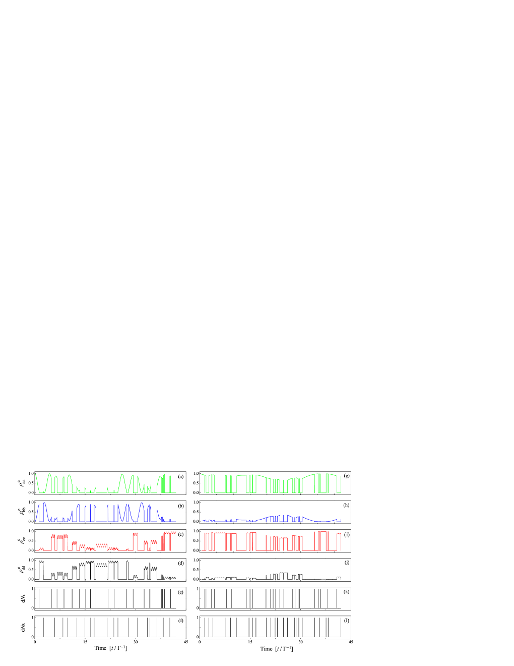
Figure 2: Typical quantum trajectories and corresponding detection records for $\Omega/\Gamma=1.0$ (a)-(f) and $\Omega/\Gamma=0.1$ (g)-(l), where $\Gamma=\Gamma_{\rm L}+\Gamma_{\rm R}$ is supposed to be a constant, and is used as the unit of energy. The initial condition is an empty SET QD with the qubit in the logical state $\alpha$ as shown in Fig. 1(a), i.e., $\rho^{\rm c}(t=0)=|{\rm a}\rangle\langle{\rm a}|$. The measurement voltage is $V/\Gamma=5$ ($\mu_{\rm L/R}=\pm 2.5\Gamma$), such that $\lambda_{+}>\mu_{\rm L}>\lambda_{-}>\mu_{\rm R}$. The involving Fermi functions can be well approximated by either one or zero. The time step used is $\Delta t$=0.01$\Gamma^{-1}$. Other plotting parameters are: $\epsilon=0$, $k_{\rm B}T/\Gamma=1.0$, $\Gamma_{\rm L}=\Gamma_{\rm R}=\Gamma/2$, and $\delta U/\Gamma=10$.

The possible four electron configurations of the reduced quantum system (qubit plus SET) is shown schematically in Fig. 1. The eigenenergies for a symmetric qybit ($\epsilon=0$) can be readily obtained as $\lambda_{+}\pm\Omega$ and $\lambda_{-}\pm\Omega$, where $\lambda_{\pm}=\frac{1}{2}(\delta U\pm\sqrt{\delta U^{2}+\Omega^{2}})$. Here, we consider the case of $\delta U\gg\Omega$. Then the eigenenergies may be greatly simplified, i.e. $\lambda_{+}\pm\Omega\approx\lambda_{+}$ and $\lambda_{-}\pm\Omega\approx\lambda_{-}$. Under the application of an appropriate bias voltage $\lambda_{+}>\mu_{\rm L}>\lambda_{-}>\mu_{\rm R}$, the involving Fermi functions in the tunneling rates are approximated by either one or zero, and the resultant quantum master equation describing the reduced dynamics can be remarkably simplified. Let us denote the density matrix elements by $\rho_{jj^{\prime}}$ where $j,j^{\prime}=\{{\rm a,b,c,d}\}$ corresponds to one of the electron configurations as shown in Fig. 1(a)-(d), respectively. The $\chi$-resolved quantum master equation (IV) reads

$$\frac{\partial}{\partial t}\tilde{\rho}_{\rm aa}= {\rm i}\Omega(\tilde{\rho}_{\rm ab}-\tilde{\rho}_{\rm ba})-\Gamma_{\rm L}\tilde{\rho}_{\rm aa}+e^{{\rm i}\chi_{\rm R}}\Gamma_{\rm R}\tilde{\rho}_{\rm cc},$$ (19a)

$$\frac{\partial}{\partial t}\tilde{\rho}_{\rm bb}= {\rm i}\Omega(\tilde{\rho}_{\rm ba}-\tilde{\rho}_{\rm ab})+(e^{{\rm i}\chi_{\rm L}}\Gamma_{\rm L}+e^{{\rm i}\chi_{\rm R}}\Gamma_{\rm R})\tilde{\rho}_{\rm dd},$$ (19b)

$$\frac{\partial}{\partial t}\tilde{\rho}_{\rm cc}= {\rm i}\Omega(\tilde{\rho}_{\rm cd}-\tilde{\rho}_{\rm dc})+e^{-{\rm i}\chi_{\rm L}}\Gamma_{\rm L}\tilde{\rho}_{\rm aa}-\Gamma_{\rm R}\tilde{\rho}_{\rm cc},$$ (19c)

$$\frac{\partial}{\partial t}\tilde{\rho}_{\rm dd}= {\rm i}\Omega(\tilde{\rho}_{\rm dc}-\tilde{\rho}_{\rm cd})-(\Gamma_{\rm L}+\Gamma_{\rm R})\tilde{\rho}_{\rm dd},$$ (19d)

$$\frac{\partial}{\partial t}\tilde{\rho}_{\rm ab}= {\rm i}\Omega(\tilde{\rho}_{\rm aa}-\tilde{\rho}_{\rm bb})+{\rm i}\Lambda(\tilde{\rho}_{\rm ab}-\tilde{\rho}_{\rm cd})-\frac{1}{2}\Gamma_{\rm L}\tilde{\rho}_{\rm ab}$$

$$+\left(\frac{1}{2}e^{{\rm i}\chi_{\rm L}}\Gamma_{\rm L}+e^{{\rm i}\chi_{\rm R}}\Gamma_{\rm R}\right)\tilde{\rho}_{\rm cd},$$ (19e)

$$\frac{\partial}{\partial t}\tilde{\rho}_{\rm cd}= {\rm i}\Omega(\tilde{\rho}_{\rm cc}-\tilde{\rho}_{\rm dd})-{\rm i}\Lambda(\tilde{\rho}_{\rm ab}-\tilde{\rho}_{\rm cd})+\frac{1}{2}e^{-{\rm i}\chi_{\rm L}}\Gamma_{\rm L}\tilde{\rho}_{\rm ab}$$

$$+\left(-\frac{1}{2}\Gamma_{\rm L}-\Gamma_{\rm R}+{\rm i}\delta U\right)\tilde{\rho}_{\rm cd},$$ (19f)

where $\Lambda$, the renormalization of qubit level mismatch arising from bath spectral functions [cf. Eq. (8)], is given by Luo et al. (2010)

$$\Lambda=\sum_{\ell={\rm L},{\rm R}}\sum_{\pm}\frac{\Gamma_{\ell}}{2\pi}{\rm Re}\left[\Psi\left(\frac{1}{2}-{\rm i}\frac{\lambda_{\pm}-\mu_{\ell}}{2\pi k_{\rm B}T}\right)\right].$$ (20)

Here $\Psi$ is the digamma function, $\mu_{\ell}$ is the chemical potential of left ($\ell=$L) or right ($\ell$=R) SET electrode, $k_{\rm B}$ is the Boltzmann constant, and $T$ is the temperature. It has been revealed that this renormalization has an important impact on the signal-to-noise ratio in continuous measurement of a chage qubit. Apparently, this effect is absent in the Lindblad master equation.

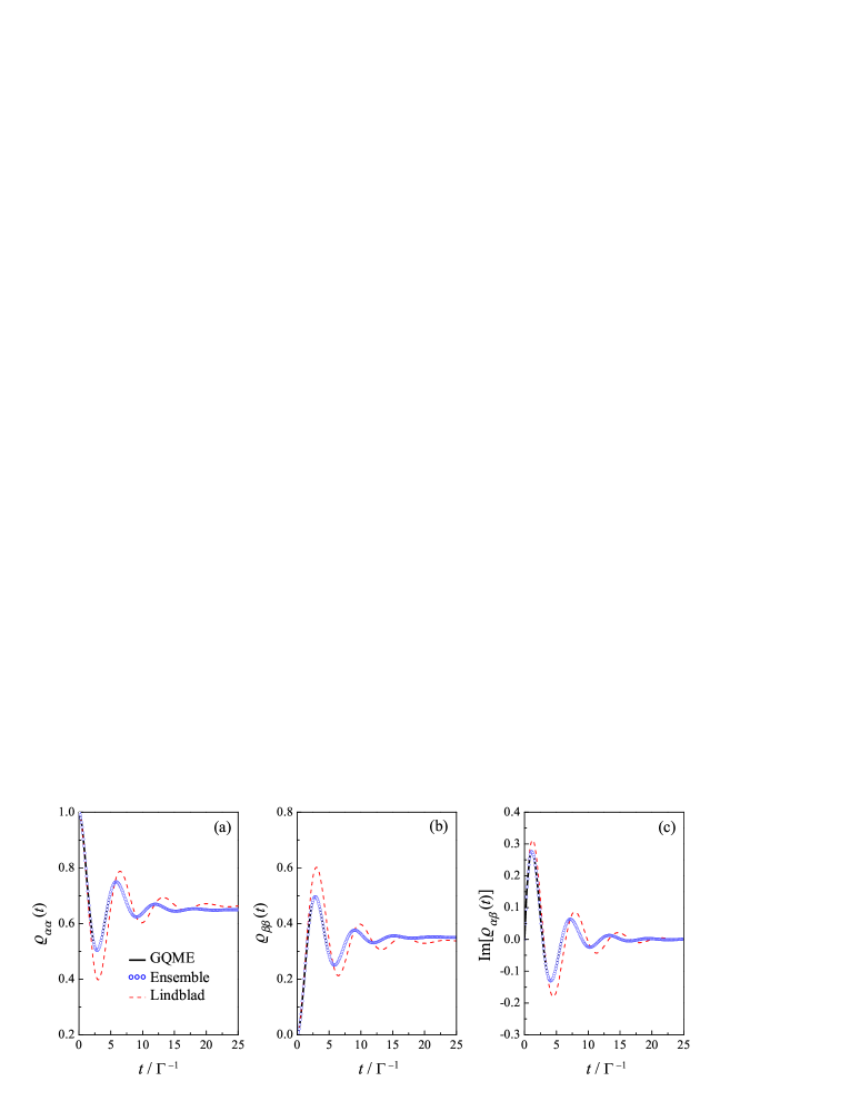
Figure 3: Unconditional measurement dynamics obtained by using the G-QMME (5) (solid curves), ensemble average over 20 thousand quantum trajectories similar to those in Fig. 2 (symbols). For comparison, the results using Lindblad master equation are also plotted by the dashed curves. The initial condition is $\rho(t=0)=|\alpha\rangle\langle\alpha|$. The total tunneling width $\Gamma=\Gamma_{\rm L}+\Gamma_{\rm R}$ is kept constant, and used as the unit of energy. Other plotting parameters used are: $\epsilon=0$, $\Omega/\Gamma=0.5$, $V/\Gamma=5$, $k_{\rm B}T/\Gamma=1$, $\Gamma_{\rm L}=\Gamma_{\rm R}=\Gamma/2$, and $\delta U/\Gamma=10$.

We are now in a position to employ the theory developed in section IV to unravel the quantum master equation (19) into individual quantum trajectories, which will be used to implement feedback control of the charge qubit later. The numerical results for conditional state evolution and corresponding tunneling events are displayed in Fig. 2 for different values of qubit interdot coupling $\Omega$. The initial condition corresponds to the charge configuration as shown in Fig. 1(a), i.e. $\rho^{\rm c}(t=0)=|{\rm a}\rangle\langle{\rm a}|$. For $\Omega/\Gamma=1.0$, the qubit exhibits oscillations between the quantum states $|{\rm a}\rangle$ and $|{\rm b}\rangle$, which is stochastically interrupted whenever one electron tunnels into the SET [see Fig. 2(e) for ${\rm d}N_{\rm L}$]. The electron may dwell on the SET for a random amount of time, where it experiences fast oscillations with frequency $\sim\lambda_{+}$, before it tunnels out of the SET QD. The conditional state evolution and corresponding tunneling events become quite different in the case of suppressed interdot coupling $\Omega/\Gamma=0.1$. One observes very slow oscillations between $|{\rm a}\rangle$ and $|{\rm b}\rangle$, as shown in Fig. 2(g)-(h). Unambiguously, we find bunching of electron tunneling events through the SET; see Fig. 2(k)-(l). When the qubit stays in the logical state $|\beta\rangle$, it will prevent electrons tunnel through the SET due to the strong Coulomb repulsion between the qubit and SET QD ($\delta U/\Gamma\gg 1$). Electrons can only flow in short time windows where the qubit relaxes to the state $|\alpha\rangle$, leading eventually to the bunching of tunneling events.

The occurrence of the bunching of tunneling events is also manifested in the FCS of SET current. By using the number-resolved quantum master equation (9), the first cumulant (current) is given by

$$\langle I\rangle=\frac{\Gamma_{\rm L}\Gamma_{\rm R}}{\Gamma_{\rm L}+2\Gamma_{\rm R}},$$ (21)

which is apparently independent of the dynamical structure of the qubit. The second cumulant $\langle I^{2}\rangle$ is associated to the shot noise. The corresponding Fano factor $F\equiv\langle I^{2}\rangle/\langle I\rangle$ is given by

$$F=\frac{\Gamma_{\rm L}^{2}+4\Gamma_{\rm R}^{2}}{(\Gamma_{\rm L}+2\Gamma_{\rm R})^{2}}+\frac{\Gamma_{\rm L}^{2}\Gamma_{\rm R}^{2}}{2(\Gamma_{\rm L}+2\Gamma_{\rm R})^{2}\Omega^{2}}+{\cal O}\left(\frac{1}{\delta U}\right),$$ (22)

which unambiguously depends on the the qubit parameter ($\Omega$). Here, the first term is simply the shot noise of a double-barrier system Blanter and Büttiker (2000); Chen and Ting (1991); Luo et al. (2007) and is definitely below the Poisson value. The influence of qubit dynamics on the SET transport is characterized by the second term. The noise may be remarkably enhanced as the qubit interdot coupling $\Omega$ decreases, leading to bunching of tunneling events as shown in Fig. 2(k)-(l). Our result thus shows unambiguously that the intrinsic dynamics of the qubit may serve as an essential mechanism that leads to bunching of tunneling events, and finally to a strong super-Poissonian noise in transport through a single QD SET.

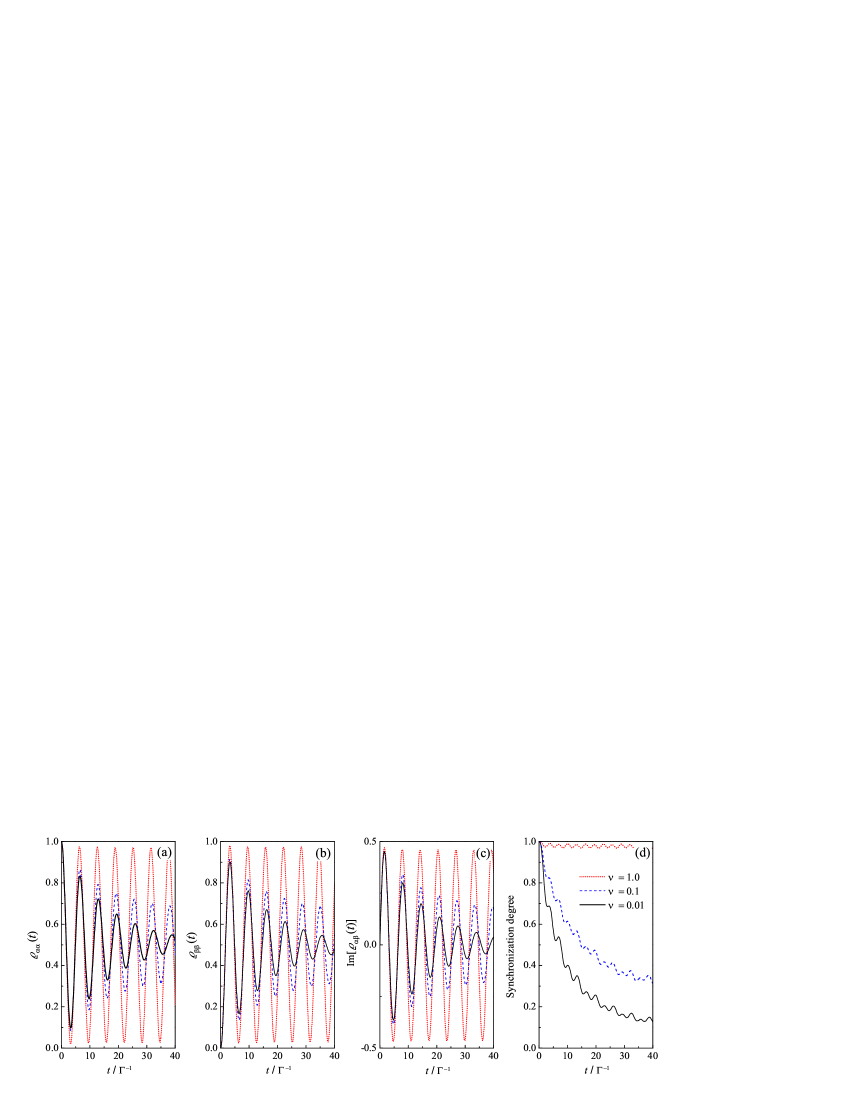
Figure 4: The dynamics of the charge qubit and corresponding degree of synchronization for different values of feedback strength $\nu=0.01$ (solid curves), $\nu=0.1$ (dashed curves), and $\nu=1.0$ (dotted curves). The results are obtained by ensemble average over 20 thousand quantum trajectories. The total tunneling width $\Gamma=\Gamma_{\rm L}+\Gamma_{\rm R}$ is constant and used as the unit of energy. Other plotting parameters used are the same as those in Fig. 3.

To further verify the validity of our Monte Carlo method for conditional evolution of the reduced state, it is instructive to make ensemble average over a large number of quantum trajectories analogous to those in Fig. 2, and then compare with the results obtained using the G-QMME (5). Yet, the G-QMME or the quantum trajectory describes the propagation of the combined (qubit plus SET QD) system. One thus has to trace over the degrees of freedom of the QD to obtain the dynamics of the qubit alone

$$\varrho(t)={\rm tr}_{\rm SET}\{\rho(t)\},$$ (23)

where ${\rm tr}_{\rm SET}\{\cdots\}$ stands for the trace over the degrees of freedom of the SET QD. One may expect perform the trace directly upon Eq. (5); Yet, a closed form of the master equation for the qubit alone cannot be obtained without further approximations. One possible method is to assume extremely asymmetric tunnel junctions for the SET and then adiabatically eliminate the degrees of freedom of the SET island to arrive at the reduced density matrix for the qubit alone Wiseman et al. (2001). Actually, such an assumption is equivalent to treating the SET effectively as a single junction detector, analogous to a quantum point contact.

Here, we first numerically propagate the combined (qubit plus SET) system, and then trace over the degrees of freedom of the SET QD, i.e. Eq. (23) to get the dynamics of the qubit alone. The numerical result is shown in Fig. 3. The reduced dynamics by using G-QMME (solid curves) and by ensemble average over 20 thousand quantum trajectories (symbols) show striking agreement, and thus verifies the validity of the unraveling scheme proposed in section IV. For comparison, the result obtained using the Lindblad master equation is also plotted by the dashed curves in Fig. 3. Notable difference is observed, which arises actually from the renormalization of the level mismatch $\Lambda$ in Eq. (20).

VI Implementation of Feedback control

So far, we have presented a Monte Carlo method to simulate the continuous quantum measurement of a charge qubit by an SET detector. Now we are in a position to implement the feedback control of coherent evolution of the charge qubit by utilizing the unraveling of the underlying measurement dynamics governed by the G-QMME, which is not necessarily of non-Lindblad form. In the dot state of the qubit ($|\alpha\rangle$ and $|\beta\rangle$), the desired (target) pure state under protect is

$$|\psi_{\rm d}(t)\rangle=\cos(\Omega t)|\alpha\rangle+{\rm i}\sin(\Omega t)|\beta\rangle$$ (24)

where $\Omega$ is the inherent qubit interdot coupling.

The basic idea of the feedback is to convert the detector’s output into the evolution of a qubit state $\varrho_{\rm c}(t)$, with $\varrho^{\rm c}(t)={\rm tr}_{\rm SET}\{\rho_{\rm c}(t)\}$. The real-time state $\varrho^{\rm c}(t)$ is then compared with the desired state $\varrho_{\rm d}(t)\equiv|\psi_{\rm d}(t)\rangle\langle\psi_{\rm d}(t)|$, their difference is utilized to design the feedback Hamiltonian such that their difference can be reduced in the next evolution step. In each successive step, the feedback Hamiltonian acts only for an infinitesimal time interval ${\rm d}t$. According to the suboptimal algorithm Doherty et al. (2001), state propagation in each infinitesimal time step maximizes the fidelity of $\varrho^{\rm c}(t)$ with $\varrho_{\rm d}(t)$. Specifically, let us consider state evolution concerning the feedback Hamiltonian, the state $\varrho^{\rm c}(t+{\rm d}t)$ is given by

$$\varrho^{\rm c}(t+{\rm d}t)= \varrho^{\rm c}(t)-{\rm i}[H_{\rm fb},\varrho^{{\rm c}}(t)]{\rm d}t$$

$$-\frac{1}{2}[H_{\rm fb},[H_{\rm fb},\varrho^{\rm c}(t)]]({\rm d}t)^{2}+\cdots,$$ (25)

where the feedback Hamiltonian $H_{\rm fb}$ is to be determined via corresponding restrictions.

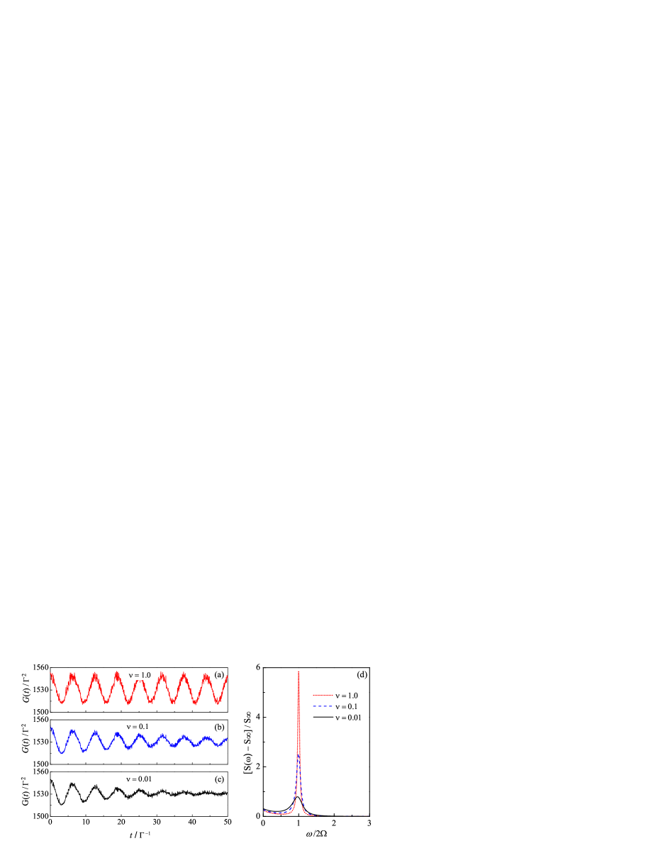
Figure 5: Correlation functions of transport current through the left junction and the corresponding noise spectrum for different values of feedback strength $\nu=0.01$ (solid curves), $\nu=0.1$ (dashed curves), and $\nu=1.0$ (dotted curves). The correlations are obtained by ensemble average over 8,000 quantum trajectories. The total tunneling width $\Gamma=\Gamma_{\rm L}+\Gamma_{\rm R}$ is set as the unit of energy. Other plotting parameters are the same as those in Fig. 3.

The fidelity of the state $\varrho^{\rm c}(t+{\rm d}t)$ with the target state then is simply given by

$${\rm Fid}\equiv \langle\psi_{\rm d}|\varrho^{\rm c}(t+{\rm d}t)|\psi_{\rm d}\rangle$$

$$= \langle\psi_{\rm d}|\varrho^{\rm c}(t)|\psi_{\rm d}\rangle-{\rm i}\langle\psi_{\rm d}|[H_{\rm fd},\varrho^{\rm c}(t)]|\psi_{\rm d}\rangle{\rm d}t$$

$$-{\textstyle\frac{1}{2}}\langle\psi_{\rm d}|[H_{\rm fb},[H_{\rm fb},\varrho^{\rm c}(t)]]|\psi_{\rm d}\rangle({\rm d}t)^{2}+\cdots.$$ (26)

To optimize the fidelity, one should maximize the dominant term, i.e. the one proportional to ${\rm d}t$. This imposes certain constraints, e.g. the sum of the squares of the eigenvalues, the sum of the norms of the eigenvalues, or the restriction on the maximum eigenvalue of $H_{\rm fb}$, etc. Actually, these constraints originate from the limitation on the feedback strength or finite Hamiltonian resources. By employing the first type of constraint, i.e. ${\rm tr}_{\rm qb}\{H^{2}_{\rm fb}\}\leq\nu$ with ${\rm tr}_{\rm qb}\{\cdots\}$ the trace over the qubit states, the feedback Hamiltonian is constructed as Wang et al. (2007); Jin et al. (2006)

$$H_{\rm fb}={\rm i}\kappa[|\psi_{\rm d}(t)\rangle\langle\psi_{\rm d}(t)|,\varrho^{{\rm c}}(t)],$$ (27)

where $\kappa=\sqrt{\frac{\nu}{2(p-q)}}$, with $p=\langle\psi_{\rm d}|[\varrho^{\rm c}(t)]^{2}|\psi_{\rm d}\rangle$ and $q=[\langle\psi_{\rm d}|\varrho^{\rm c}(t)|\psi_{\rm d}\rangle]^{2}$.

To make it much more easily accessible for experimentalists to implement the above feedback control protocol, we insert Eq. (24) into Eq. (27), and eventually arrive at a translation of the feedback Hamiltonian as

$$H_{\rm fb}=K\sigma_{x}$$ (28)

with

$$K=\left\{\begin{array}[]{ll}+\sqrt{\frac{\nu}{2}},&\Delta\phi<0\\ -\sqrt{\frac{\nu}{2}},&\Delta\phi>0\end{array}.\right.$$ (29)

It resembles a simple bang-bang control, where the feedback parameter between two values is simply determined by the phase “error” defined as $\Delta\phi\equiv\phi(t)-\phi_{0}$, with $\phi(t)=\arctan(2{\rm Im}\{\varrho^{\rm c}_{\alpha\beta}(t)\}/[\varrho^{\rm c}_{\alpha\alpha}(t)-\varrho^{\rm c}_{\beta\beta}(t)])$ the relative phase between the logical states “$|\alpha\rangle$” and “$|\beta\rangle$”, and $\phi_{0}=2\Omega t$(mod $2\pi$). It is worthwhile to mention that the two versions of the feedback Hamiltonian protocols, i.e. Eq. (27) and Eq. (28) are totally equivalent to each. Yet, second one actually provided a much easier way for experimentalists to implement.

In Fig. 4, the effect of feedback control is plotted for various values of feedback strength $\nu$. The feedback is implemented into every single quantum trajectories, analogous to those in Fig. 2. Eventually the propagation of the state is obtained by an ensemble average over 20 thousand trajectories. For sufficient large feedback strength (see the dotted curves for $\nu$=1), coherent oscillation of the charge quit can be maintained, in principle, for an arbitrarily long time. To quantitatively characterize how close to the desired state the protected state reach, we introduce the synchronization degree, defined as $D\equiv 2{\rm tr}_{\rm qb}\{\varrho^{\rm c}\varrho_{\rm d}\}-1$. For $D=1$, it means complete synchronization, indicating that the state is perfectly protected via the feedback control. The results for various feedback strengths are shown in Fig. 4(d). Apparently, for a large feedback strength ($\nu=1$), the synchronization degree can reach almost the maximum value of 1, showing thus the high effectiveness of our feedback scheme.

Another important figure of merit of the coherent oscillations is the signal-to-noise ratio of the detector’s output. To investigate this important feature of feedback effect, we first evaluate the correlation function of current transport through the left junction of the SET (the right one gives similar results) according to Eq. (17). The numerical results obtained by ensemble average over 8,000 quantum trajectories are displayed in Fig. 5 for different feedback strength $\nu$. As $\nu$ increases, the correlation function demonstrates clearly coherent oscillation behavior; see Fig. 5(a) for $\nu=1.0$. With the knowledge of the current correlation function, the corresponding noise spectrum can be obtained directly by performing the Fourier transformation, as shown in Eq. (18). The numerical results are shown in Fig. 5(d). An enhancement of the feedback strength leads to a rising and sharping of the coherent peak located at frequency $\omega=2\Omega$. Actually, the height of this peak relative to its pedestal is a measure of the signa-to-noise ratio. It was argued in that the signal-to-noise ratio is limited at 4, known as the Korotkov-Averin bound Korotkov (2001b); Korotkov and Averin (2001). It was revealed the signal-to-noise ratio of an SET detector can not reach the limit of an ideal detector Gurvitz and Berman (2005). However, we find the signal-to-noise ratio can be remarkably increased in the case of strong feedback strength (see the dotted curve), even violating Korotkov-Averin bound. Our feedback protocol thus serves an effective method to improve the signal-to-noise ratio that can exceed the up bound limit of 4, indicating ideal qubit coherent oscillations under continuous measurement by an SET detector.

Recently, a closed-loop feedback scheme was proposed for the stabilization of a pure qubit state by employing, analogously, a capacitively coupled SET. There, the real-time tunneling events through SET detector was directly back-coupled into qubit parameters. This purification process was found to be independent of the initial state and could be accomplished simply after a few electron jumps through the SET detector. The qubit states is stabilized above a critical detector-qubit coupling. In comparison, the advantage of our feedback scheme is that a coherent oscillations of the qubit could be maintained for arbitrary qubit parameters, as long as the feedback strength is sufficient strong.

VII Summary

In the context of a charge qubit under continuous monitoring by a single electron transistor, we have proposed an unraveling scheme of the G-QMME into an ensemble of individual quantum trajectories specifically for stochastic point process. A suboptimal feedback algorism is implemented into every single quantum trajectory to protect a desired pure state. It is demonstrated that coherent oscillation of the charge qubit can be maintained for an arbitrarily long time in the case of sufficient feedback strength. The corresponding synchronization degree can reach almost close to the maximum value of 1. It is also observed that the signal-to-noise ratio increases with rising feedback strength, and remarkably could even exceed the well-known Korotkov-Averin bound in quantum measurement, reflecting actually ideal quantum coherent oscillations of the qubit. The proposed unraveling and feedback scheme thus may serve as an essential mechanism to sustain ideal quantum coherent oscillations in a very transparent and straightforward manner. It is also highly expect that it may have important applications in the field of solid-state in quantum computational algorithms.