Recharging Probably Keeps Batteries Alive

Abstract

The kinetic battery model is a popular model of the dynamic behavior of a conventional battery, useful to predict or optimize the time until battery depletion. The model however lacks certain obvious aspects of batteries in-the-wild, especially with respect to $(\mathit{i})$ the effects of random influences and $(\mathit{ii})$ the behavior when charging up to capacity bounds.

This paper considers the kinetic battery model with bounded capacity in the context of piecewise constant yet random charging and discharging. The resulting model enables the time-dependent evaluation of the risk of battery depletion. This is exemplified in a power dependability study of a nano satellite mission.

1 Introduction

The kinetic battery model (KiBaM) is a popular representation of the dynamic behavior of the state-of-charge (SoC) of a conventional rechargeable battery [24, 25]. Given a constant load, it characterizes the battery SoC by two coupled differential equations. Empirical evaluations show that this model provides a good approximation of the SoC across various battery types [20, 21].

The original KiBaM does not take capacity bounds into considerations, it can thus be interpreted as assuming infinite capacity. Reality is unfortunately different. When studying the KiBaM operating with capacity bounds, it becomes apparent that charging and discharging are not dual to each other. However, opposite to the discharging process, the charging process near capacity bounds has not received dedicated attention in the literature. That problem is attacked in the present paper.

Furthermore, statistical results obtained by experimenting with real of-the-shelf batteries suggest considerable variances in actual performance [5], likely rooted in manufacturing and wear differences. This observation asks for a stochastic re-interpretation of the classical KiBaM to take the statistically observed SoC spread into account on the model level, and this is what the present paper develops – in a setting with capacity bounds. It views the KiBaM as a transformer of the continuous probability distribution describing the SoC at any real time point, thereby also supporting uncertainty and noise in the load process.

The approach presented not only enables the treatment of randomness with respect to the battery itself, but also makes it possible to determine the SoC distribution after a sequence of piecewise constant, yet random charge or discharge loads. We develop the approach in a setting with continuous randomness so as to directly support normal (i.e. Gaussian), Weibull or exponential distributions. We apply the model to a case study inspired by a nano satellite currently orbiting the earth [17], for which we need to superpose it with a periodic deterministic charge load, representing the infeed from on-board solar panels.

The resulting battery model can be viewed as a particular stochastic hybrid system [1, 2, 3, 6, 9, 28], developed without discretizing time. It can (for instance) for any given real time point provide probabilistic guarantees about the battery never being depleted before.

The genuine contributions of the paper are: $(\mathit{i})$ The interpretation of the KiBaM as a transformer of SoC distributions, $(\mathit{ii})$ developed without discretizing time, $(\mathit{iii})$ considering both charging and discharging in the context of capacity bounds, $(\mathit{iv})$ applied to a case study of a low earth orbiting satellite.

Related work

Haverkort and Jongerden [21] review broad research on various battery models. They discuss stochastic battery models [25, 7] which view the KiBaM for a given load as a stochastic process, unlike our (more accurate) view as a deterministic transformer of the randomized initial conditions of the battery. Furthermore, in this survey, the problem of charging bounds does not get dedicated attention.

Battery capacity has been addressed only by Boker et al. [4]. They considered a discretized, unbounded KiBaM together with a possibly non-deterministic and cyclic load process, synthesizing initial capacity bounds to power the process safely. Hence, capacity is here understood as an over-dimensioned initial condition and not as a truly limiting charging bound.

Random loads on a battery, generated by a continuous-time Markov chain, have been previously studied by Cloth et al. [7]. Their setting cannot be easily extended by charging since they view the available and bound charge levels as two types of accumulated reward in a reward-inhomogeneous continuous time Markov chain.

An extension of the KiBaM to scheduling has been considered by Jongerden et al. [19]. They compute optimal schedules for multiple batteries in a discretized setting with only discharging. This has been taken up and improved using techniques from the planning domain [12].

2 The Kinetic Battery Model

The kinetic battery model is a mathematical characterization of the state of charge of a battery. It differs from an ideal energy source by incorporating the fact that not all the energy stored in a battery is available at all times. The stored energy is divided into two portions, the available charge and the bound charge. Only the available charge may be consumed immediately by a load supported by the battery and thereby behaves similar to an idealized source. As time passes, some of the bound charge is converted into available charge and is thus free to be consumed. This effect is coined the recovery effect as the available charge recovers to some extend during periods of low discharge or no discharge at all. The recovery effect agrees with our experiences using batteries: For instance, when a cellphone switches off due to an apparently empty battery, it often can be switched back on after waiting a few minutes. The battery seems to have recovered. This diffusion between available and bound charge can take place in either direction depending on the amount of both types of energy stored in the battery. Thus, while charging the battery, available charge is converted to bound charge. This behavior is illustrated by Figure 1.

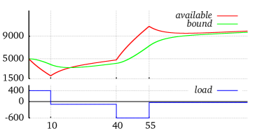
Figure 1: Evolution of the state of charge as time passes (top) with the battery strained by a piecewise-constant load (bottom). The initially available charge decreases heavily due to the load $400$ but the restricted diffusion makes the bound charge decrease only slowly up to time $10$; after that the battery undergoes a mild recharge, followed by a strong recharge and a mild recharge at the end. At all times the bound charge approaches the available charge by a speed proportional to the difference of the two values.

Coupled differential equations

The KiBaM is often depicted as two wells holding liquid, the available charge and the bound charge well, interconnected by a pipe that represents the diffusion of the two types of charge, see Figure 2.

Figure 2: The two-well-model of the KiBaM with the available charge on the right (exposed directly to the load $I$) connected to the bound charge on the left by a pipe of width $p$.

Formally, the KiBaM is characterized by two coupled differential equations.

$$\dot{a}(t) = -I+p\left(\frac{b(t)}{1-c}-\frac{a(t)}{c}\right)$$ (1)

$$\dot{b}(t) = p\left(\frac{a(t)}{c}-\frac{b(t)}{1-c}\right)$$ (2)

Here, the functions $a(t)$ and $b(t)$ describe the available and bound charge respectively, $I$ is a load on the battery, $p$ is the diffusion rate between both wells and $c$ is the width of the available charge well. Thus $1-c$ is the width of the bound charge well. Intuitively $a(t)/c$ and $b(t)/(1-c)$ are the level of the fluid stored in the available charge well and the bound charge well, respectively. By defining

$$k=\dfrac{p}{c(1-c)}$$

we can rewrite (1) and (2) to

$$\dot{a}(t) = -I+ck\cdot b(t)-(1-c)k\cdot a(t)$$

$$\dot{b}(t) = (1-c)k\cdot a(t)-ck\cdot b(t).$$

We will use this version of the KiBaM ODEs throughout this paper.

Solving the equations

Using Laplace transforms the KiBaM ODE system can be solved, arriving at

$$a_{t,I}(a_{0},b_{0}) = \mathrm{q}_{a}(t)a_{0}+\mathrm{r}_{a}(t)b_{0}+\mathrm{s}_{a}(t)I$$

$$b_{t,I}(a_{0},b_{0}) = \mathrm{q}_{b}(t)a_{0}+\mathrm{r}_{b}(t)b_{0}+\mathrm{s}_{b}(t)I$$

where $a_{0}$ and $b_{0}$ are the initial available and bound charge levels and the time-dependent coefficients of $a_{0},b_{0}$ and $I$ in the equations can be expressed as

$$\mathrm{q}_{a}(t) = \phantom{-}(1-c)\mathrm{e}^{-kt}+c$$

$$\mathrm{q}_{b}(t) = -(1-c)\mathrm{e}^{-kt}+(1-c)$$

$$\mathrm{r}_{a}(t) = -c\cdot\mathrm{e}^{-kt}\hskip 16.0pt+c$$

$$\mathrm{r}_{b}(t) = \phantom{-}c\cdot\mathrm{e}^{-kt}\hskip 16.0pt+(1-c)$$

$$\mathrm{s}_{a}(t) = \frac{(1-c)(\mathrm{e}^{-kt}-1)}{k}-t\cdot c$$

$$\mathrm{s}_{b}(t) = \frac{(1-c)(1-\mathrm{e}^{-kt})}{k}-t\cdot(1-c).$$

From the solution we can see that the KiBaM is affine in $a_{0}$ and $b_{0}$ (and also $I$). Thus we can combine the two functions into one vector valued linear mapping

$$\textsc{{K}}_{t,I}\left[\begin{array}[]{c}a_{0}\\ b_{0}\end{array}\right]=\left[\begin{array}[]{ccc}\mathrm{q}_{a}(t)&\mathrm{r}_{a}(t)&\mathrm{s}_{a}(t)\\ \mathrm{q}_{b}(t)&\mathrm{r}_{b}(t)&\mathrm{s}_{b}(t)\end{array}\right]\cdot\left[\begin{array}[]{c}a_{0}\\ b_{0}\\ I\end{array}\right].$$

When $t$ is clear from context, we simplify the notation and drop the argument of these coefficients (without dropping the time-dependency). From now on we prefer semicolon notation $[a;b]$ to denote column vectors. (All vectors appearing in this paper are column vectors.) Furthermore, whenever we compare two vectors, e.g., $[a;b]\leq[a^{\prime},b^{\prime}]$, we interpret the order component-wise.

Example 1.

The function K can be used to approximate the final SoC in Figure 1 (for $k=1/100$, $c=1/2$, and $\circ$ denoting function composition) by

$$\left[a;b\right] =\textsc{{K}}_{44,100}\circ\textsc{{K}}_{15,-600}\circ\textsc{{K}}_{30,-100}\circ\textsc{{K}}_{10,400}\left[5000;5000\right]$$

$$\approx\textsc{{K}}_{44,100}\circ\textsc{{K}}_{15,-600}\circ\textsc{{K}}_{30,-100}\left[2002;3998\right]$$

$$\approx\textsc{{K}}_{44,100}\circ\textsc{{K}}_{15,-600}\left[4802;4198\right]$$

$$\approx\textsc{{K}}_{44,100}\left[10732;7268\right],$$

and with the last step in more details (denoting $$\mathrm{e}^{-\frac{44}{100}} E$$ by ),

$$=\left[\begin{array}[]{ccc}\phantom{-}\frac{1}{2}E+\frac{1}{2}&-\frac{1}{2}E+\frac{1}{2}&50E-50-\frac{44}{2}\\ -\frac{1}{2}E+\frac{1}{2}\rule{0.0pt}{11.19443pt}&\phantom{-}\frac{1}{2}E+\frac{1}{2}&50-50E-\frac{44}{2}\end{array}\right]\cdot\left[\begin{array}[]{c}10732\\ 7268\\ -35\end{array}\right]$$

$$=\left[\begin{array}[]{c}-18E+6480\\ \phantom{-}18E+8020\end{array}\right]\approx\left[\begin{array}[]{c}9881\\ 9659\end{array}\right].$$

On the last line, the first summands (with $E$) stand for the spread of the values when the recovery effect has not converged yet (as for $t\to\infty$, $E\to 0$). For $c=1/2$ and zero load, the recovery effect makes the difference of the available charge and the bound charge converge to $0$. However, for non-zero load $I$, it does not converge to $0$ but to $I/k$ which explains the difference in the second summands.

Battery Depletion

A standard application of KiBaM is to find out whether a task can be performed with a given initial state of charge without depleting the battery. A task is a pair $(T,I)$ with $T$ being the task execution time, and $I$ representing the load, imposed for duration $T$.

For an execution time $T$ and a load $I$, we say that a battery with a SoC $[a_{0};b_{0}]>[0;0]$ powers a task $(T,I)$ if

$$\textsc{{K}}_{t,I}\left[a_{0};b_{0}\right] >[0;0] \text{$\forall\;0\leq t\leq T$}.$$

Let us stress that the state of charge of the battery evolves in negative numbers in the same way as in positive numbers because the differential equations do not have any explicit bounds. To rule out that the SoC of the battery goes into negative numbers and returns back, we need a certain form of monotonicity.

Example 1 (Cont.).

We notice that neither the available nor the bound charge are monotonous in the standard sense. In Figure 1, the bound charge is not monotonous on $[10,40]$, the available charge is not monotonous on $[55,100]$. However, for instance, on $[40,55]$, available charge is the first to get above the value $9000$ (and never crosses the boundary again).

Lemma 1.

For any $\kappa,I\in\mathbb{R}$, $\preceq\;\in\{\leq,\geq\}$, and $0\leq t\leq T$,

$$\forall a_{0}\not\preceq\kappa,\forall b_{0}\not\preceq\kappa:\;\;b_{t,I}(a_{0},b_{0})\preceq\kappa\; \Longrightarrow\;a_{t,I}(a_{0},b_{0})\preceq\kappa,$$

$$\forall a_{0}\not\preceq\kappa,\forall b_{0}\not\preceq\kappa:\;\;a_{t,I}(a_{0},b_{0})\preceq\kappa\; \Longrightarrow\;a_{T,I}(a_{0},b_{0})\preceq\kappa.$$

Intuitively speaking, the first property states that the available charge is always the first to cross a bound, the second property states that when the available charge crosses a bound it never returns back (for a given load).

As a direct consequence of Lemma 1, we can easily figure out whether the battery powers a task.

Lemma 2.

A battery with a SoC $[a_{0};b_{0}]>[0;0]$ powers a task $(T,I)$ if and only if $\textsc{{K}}_{T,I}\left[a_{0};b_{0}\right]>[0;0]$.

3 The Basic Random KiBaM

Some basic notions from probability theory are needed for the further development. Let $f_{X}$ and $f_{X\times Y}$ denote the density function of a random variable $X$ and the joint density function of a pair of random variables $(X,Y)$, respectively.

The conditional density function $f_{X\mid Y}$ of $X$ given the occurrence of the value $y$ of $Y$ is defined as $f_{X\mid Y}(x|y)=f_{X\times Y}(x,y)/f_{Y}(y)$. From this expression for $f_{X\times Y}$, we obtain by marginalization the density function $f_{X}$ as

$$f_{X}(x)=\int_{-\infty}^{\infty}f_{X\mid Y}(x|y)f_{Y}(y)~{}\mathrm{d}y.$$ (3)

Furthermore, the transformation law for random variables enables the construction of unknown density functions from known ones given the relation between the corresponding random variables. Formally, for every $d$-dimensional random vector $\mathbf{X}$ and every injective and continuously differentiable function $g:\mathbb{R}^{d}\to\mathbb{R}^{d}$, we can express the density function of $\mathbf{Y}:=g(\mathbf{X})$ at value $y$ in the range of $g$ as

$$f_{\mathbf{Y}}(y)=f_{\mathbf{X}}\left(g^{-1}(y)\right)\cdot\left|\textrm{{det}}\left(J_{g^{-1}}(y)\right)\right|$$ (4)

where $J_{f}(x)$ denotes the Jacobian of a mapping $f$ evaluated at $x$. Let us recall that the Jacobian of $f$ is the matrix of the partial derivatives of the mapping $f$.

Joint Density of the State of Charge

In order to consider the KiBaM as a stochastic object, it appears natural to consider the vector $[a_{0};b_{0};I]$ as being random. This naturally reflects the situation where the initial state of the battery is subject to perturbations due to manufacturing or wear variances, and so is its load. Therefore, we assume the initial SoC is expressed by random variables $A_{0},B_{0}$ endowed with a joint probability density function $f_{0}$ and that the load on the battery is expressed by a random variable $I$ endowed with a probability density function $g$. We assume that the random variables $I$ and $(A_{0},B_{0})$ are independent.

Example 2.

A second running example addresses the random KiBaM. Instead of a single (Dirac) SoC, we now assume that the joint density $f_{0}$ of the charge is, say, uniform over the area $[4,6.5]\times[4,6.5]$ (below).

We shall illustrate our findings how the SoC distribution evolves as the time passes on this particular example.

Let $(A_{T},B_{T})$ denote the random variables expressing SoC after time $T$ of constant (but random) load $I$. We are interested in the joint probability distribution of $(A_{T},B_{T})$ Thus, for a given time point $T$ we want to establish the joint density function of the vector $[A_{T};B_{T}]$ given by

$$\left[\begin{array}[]{c}A_{T}\\ B_{T}\\ \end{array}\right]=\left[\begin{array}[]{ccc}\mathrm{q}_{a}&\mathrm{r}_{a}&\mathrm{s}_{a}\\ \mathrm{q}_{b}&\mathrm{r}_{b}&\mathrm{s}_{b}\end{array}\right]\cdot\left[\begin{array}[]{c}A_{0}\\ B_{0}\\ I\end{array}\right].$$ (5)

Expressing the joint density using direct application of the transformation law for random variables is not possible because the mapping is not invertible. However, using the fact that $I$ and $(A_{0},B_{0})$ are independent, it is still possible to use the transformation law of random variables so that ultimately we arrive at an analytic characterization of the joint density of $(A_{T},B_{T})$.

In the following we will derive the conditional density of $(A_{T},B_{T})$ under the condition that $I=i$ for some arbitrary but fixed value $i$. As $g$ is known, we afterwards accommodate for the missing information about $I$ via integration over the range of $I$. Knowing that $I=i$ eliminates one source of randomness, (5) can be rewritten to

$$\left[\begin{array}[]{c}A_{T}\\ B_{T}\\ \end{array}\right]=\left[\begin{array}[]{cc}\mathrm{q}_{a}&\mathrm{r}_{a}\\ \mathrm{q}_{b}&\mathrm{r}_{b}\end{array}\right]\cdot\left[\begin{array}[]{c}A_{0}\\ B_{0}\end{array}\right]+\left[\begin{array}[]{c}\mathrm{s}_{a}\\ \mathrm{s}_{b}\end{array}\right]\cdot i$$

which is an invertible linear mapping and thus allows to express the joint density of $(A_{T},B_{T})$ in terms of the density of $(A_{0},B_{0})$ via the transformation law of random variables.

Inverting this mapping $\textsc{{K}}_{T,i}$ results in

$$\textsc{{K}}_{T,i}^{-1}\left[\begin{array}[]{c}a\\ b\\ \end{array}\right]=\mathrm{e}^{kT}\left[\begin{array}[]{ccc}\mathrm{r}_{b}&-\mathrm{r}_{a}&\mathrm{r}_{a}\mathrm{s}_{b}-\mathrm{r}_{b}\mathrm{s}_{a}\\ -\mathrm{q}_{b}&\mathrm{q}_{a}&\mathrm{q}_{b}\mathrm{s}_{a}-\mathrm{q}_{a}\mathrm{s}_{b}\end{array}\right]\cdot\left[\begin{array}[]{c}a\\ b\\ i\end{array}\right].$$

By a straightforward computation, the determinant of the Jacobian of $\textsc{{K}}_{T,i}^{-1}$ is $\textrm{{det}}{J_{\textsc{{K}}_{T,i}^{-1}}}=\mathrm{e}^{kT}$. Note that it is constant in $a$, $b$, and $i$, it only depends on $T$. Thus, using (4) we arrive at the joint density of $(A_{T},B_{T})$ conditioned by $I=i$

$$f_{T}(a,b\mid i)= f_{\textsc{{K}}_{T,i}[A_{0};B_{0}]}(a,b)$$

$$= f_{0}\left(\textsc{{K}}_{T,i}^{-1}[a;b]\right)\cdot\left|\mathrm{e}^{kt}\right|$$

where $f_{\textsc{{K}}_{T,i}[A_{0};B_{0}]}$ denotes the joint density of the random vector $\textsc{{K}}_{T,i}[A_{0};B_{0}]$. According to (3) we arrive at the unconditional density over $(A_{T},B_{T})$ via integration on $i$:

Lemma 3.

Let $T$ be execution time and $g$ be load density. For an initial SoC $f_{0}$ over $(A_{0},B_{0})$ and task $(T,g)$, the joint distribution of $(A_{T},B_{T})$ is absolutely continuous with density $f_{T}$ given by

$$f_{T}(x,y) =\int_{-\infty}^{\infty}f_{0}\left(\textsc{{K}}_{T,i}^{-1}[x;y]\right)\cdot\mathrm{e}^{kT}\cdot g(i)~{}\mathrm{d}i.$$

Example 2 (Cont.).

We return to our example assuming the density $g$ of the load being uniform between $[-0.1,0.1]$. Based on the expression from Lemma 3, we can compute the SoC of the battery after task $(20,g)$, displayed on the left, and $(60,g)$, displayed on the right. We arbitrarily chose the parameters $c=0.5$ and $p=0.002$.
 

Risk of Depletion

Let us transfer the problem of battery depletion into the stochastic setting. We say that a density $f_{0}$ is positive if for any $a,b$ such that either $a\leq 0$ or $b\leq 0$ we have $f_{0}(a,b)=0$. For an execution time $T>0$ and a load density $g$, we say that the battery with positive SoC $f_{0}$ powers with probability $p>0$ a task $(T,g)$ if

$$\mathrm{\mathbf{Pr}}\left[\forall 0\leq t\leq T:(A_{t},B_{t})>(0,0)\right]\;\geq\;p.$$

Due to the monotonicity of KiBaM from Lemma 1, this is equivalent to observing the probability of being empty only at time $T$. From Lemma 3 we obtain the following.

Lemma 4.

A battery with SoC $f_{0}$ powers with probability $p>0$ a task $(T,g)$ if and only if

$$\int_{0}^{\infty}\int_{0}^{\infty}f_{T}(a,b)~{}\mathrm{d}b~{}\mathrm{d}a\;\geq\;p.$$

Example 2 (Cont.).

Thanks to the lemma, it suffices to perform the integration on the densities displayed in the previous plots in this running example. The probability to power the tasks $(20,g)$ is $1$, for the task $(60,g)$ it is just $\approx 0.968$.

4 Bounded Recharging

For the evaluation of the long-run state of a battery, a good understanding of the charging process is as essential as understanding the discharging process. Both are well supported by the theory developed so far, and have occurred in our examples in the form of negative loads. What is not treated in the theory yet is a capacity bound of the battery which is a real constraint in most applications. To the best of our knowledge, charging in KiBaM while respecting its capacity restrictions has not been addressed even in the deterministic case. This is what we are going to develop first, and then extend to the randomized setting.

Let us assume that the battery has capacity $d$ divided into capacity $a_{\max}=c\cdot d$ of the available charge well and capacity $b_{\max}=(1-c)\cdot d$ of the bound charge well.

Charging at full available charge

A battery with empty available charge can no longer support its task. Notably, a battery with full available charge does not behave dual to the behavior at empty available charge, just because a battery with full available charge continues to operate, and we thus need to consider its further charging. In this discussion we do not consider crystallization effects reported for some batteries when overcharging [5, 26]. These phenomena do affect battery wear, not considered in our modeling efforts thus far.

When the available charge reaches its capacity $a_{\max}=c\cdot d$ and is still charged further by (high enough) incoming current, its value stays constant and only the bound charge increases due to diffusion. Hence, we know that $\dot{a}(t)=0$ and $\frac{a(t)}{c}=d$ and we can thus modify (2) to

$$\dot{b}(t) =p\left(d-\frac{b(t)}{1-c}\right).$$ (2’)

Note that this equation describes the behavior of the battery at time $t$ only if the load satisfies

$$-I\geq\dot{b}(t).$$

Since $I$ is constant and the diffusion is decreasing over time, the inequality holds for all $t$, provided

$$-I\geq\dot{b}(0)=p\left(d-\frac{b(0)}{1-c}\right),$$

or equivalently if $b(0)\geq b_{\mathrm{tresh}}(I)$ where

$$b_{\mathrm{tresh}}(I)=b_{\max}+I\cdot\frac{1-c}{p}.$$ (6)

For a smaller initial bound charge, the standard differential equations (1) and (2) apply, until the available charge hits the capacity bound again. Finally, solving the ODE (2’) yields

Lemma 5.

Let $T$ be an execution time, $I$ be a load, and $b_{0}$ be a bound charge such that $b_{0}\geq b_{\mathrm{tresh}}(I)$. A battery with a SoC $(a_{\max},b_{0})$ reaches after the task $(T,I)$ the state of charge $(a_{\max},\bar{b}_{T}(b_{0}))$ where

$$\bar{b}_{T}(b_{0})=\mathrm{e}^{-ckT}b_{0}+\left(1-\mathrm{e}^{-ckT}\right)\cdot b_{\max}$$ (7)

and $k$ again stands for $p/\left(c\cdot(1-c)\right)$.

We notice that the resulting bound charge $\bar{b}_{T}(b_{0})$ does not further depend on $I$, i.e. one cannot make the battery charge faster by increasing the charging current. Furthermore, for a fixed $b_{0}$, the curve of $t\mapsto\bar{b}_{t}(b_{0})$ is a negative exponential starting from the point $b_{0}$ with the full capacity $b_{\max}$ of the bound charge being its limit. Thus, Lemma 5 also reveals that the bound charge in finite time never gets full and there is no need to describe this situation separately. Finally, we denote analogously by $\bar{\textsc{{K}}}_{T}\left[a_{0};b_{0}\right]=\left[a_{0};\bar{b}_{T}(b_{0})\right]$ the linear mapping describing the behavior at the upper bound.

Example 1 (Cont.).

If we put an upper bound of $9000$ to the battery scenario from Figure 1, the battery ends up with a slightly smaller charge at time $100$.

Hitting the capacity bound

For a given constant load $I$, we have seen two types of behavior of the battery: ($i$) before it hits the available charge capacity and ($\mathit{ii}$) after it hits the capacity. The remaining question is when it hits the capacity limit. For a given initial state $(a_{0},b_{0})$ and a load $I$, this amounts to solving

$$a_{t,I}(a_{0},b_{0})=a_{\max},$$

which in turn yields an equation

$$u\cdot\mathrm{e}^{-kt}+v\cdot t+w =0$$

where $u=a_{0}\left(1-c\right)-b_{0}c+(c+1)\cdot I/k$, $v=-Ic$, and $w=cd-a_{0}c-b_{0}c-(1-c)\cdot I/k$. This can be solved as

$$t=-W\left(\frac{u}{v}\cdot\mathrm{e}^{-\frac{w}{v}}\right)-\frac{w}{v}$$ (8)

where $W$ is the product log function. It has no closed form but can be arbitrarily numerically approximated[8].

Deterministic KiBaM with lower and upper bounds

All the previous building blocks allow us to express easily the SoC of a deterministic KiBaM after powering a given task $(T,I)$ when considering battery bounds. We define it as the following function:

$$\textsc{{K}}^{\Box}_{T,I}\left[a_{0};b_{0}\right]=\begin{cases}\textsc{{K}}_{T,I}\left[a_{0};b_{0}\right]&\text{if $a_{0}>0$ and }\\ &\text{$\;\;0<a_{T,I}(a_{0},b_{0})\leq a_{\max}$,}\\ \bar{\textsc{{K}}}_{t}\circ\textsc{{K}}_{\bar{t},I}\left[a_{0};b_{0}\right]&\text{if $a_{0}>0$ and }\\ &\text{$\;\;a_{T,I}(a_{0},b_{0})>a_{\max}$,}\\ \left[0;0\right]&\text{otherwise, i.e. if $a_{0}=0$}\\ &\text{\;\;or $a_{T,I}(a_{0},b_{0})<0$}\end{cases}$$

where $\bar{t}$ is the largest solution of (8) and $t=T-\bar{t}$.

The KiBaM evolution has one fundamental property we rely on heavily later: for any fixed time and load, it is monotonous with respect to starting SoC.

Lemma 6.

Let $(a,b)$ and $(a^{\prime},b^{\prime})$ be two SoCs. For every $t>0$ and for every $I\in\mathbb{R}$ it holds that

$$(a,b)\leq(a^{\prime},b^{\prime})~{}\Longrightarrow~{}\textsc{{K}}^{\Box}_{t,I}[a;b]\leq\textsc{{K}}^{\Box}_{t,I}[a^{\prime};b^{\prime}].$$

Example 1 (Cont.).

By introducing the bounds in the first running example, the computation of the final SoC changes only in the interval $[40,55]$. Here, instead of $\textsc{{K}}_{15,-6}$, we apply $\textsc{{K}}_{\bar{t},-6}$ for the first $\bar{t}\approx 7.8$ time units, followed by $\bar{\textsc{{K}}}_{15-\bar{t}}$.

The computation of the time point $\bar{t}$ is problematic, as mentioned before. An alternative to numerical approximation of the exact time point of crossing a bound is provided by the following observation: If time point $t$ is fixed, we can check whether the available charge will exceed $a_{\max}$ after $t$ time units. In this case it is possible to determine the charging current $\bar{I}$ necessary for the available charge to hit $a_{\max}$ exactly after $t$ time units, i.e. solving $a_{t,I}(a_{0},b_{0})=a_{\max}$ for $I$ instead of $t$. Let us denote the solution of this equation by $\bar{I}(a_{0},b_{0})$ for a SoC $(a_{0},b_{0})$ and conclude that it can be computed by

$$\bar{I}(a_{0},b_{0})=-\frac{\mathrm{q}_{a}}{\mathrm{s}_{a}}\cdot a_{0}-\frac{\mathrm{r}_{a}}{\mathrm{s}_{a}}\cdot b_{0}+\frac{a_{\max}}{\mathrm{s}_{a}}.$$

Such a slower charging rate $\bar{I}(a_{0},b_{0})$ allows us to define a conservative under-approximation of the exact KiBaM $\textsc{{K}}^{\Box}_{T,I}[a_{0};b_{0}]$. We replace the case $\bar{\textsc{{K}}}_{t}\circ\textsc{{K}}_{\bar{t},I}\left[a_{0};b_{0}\right]$ where the upper bound is reached by $\textsc{{K}}_{T,\bar{I}(a_{0},b_{0})}[a_{0};b_{0}]$. We will henceforth refer to this under-approximation by $\textsc{{K}}^{\approx\Box}_{T,I}$.

Lemma 7.

For any SoC $(a,b)$ we have $\textsc{{K}}^{\approx\Box}_{T,I}[a;b]\leq\textsc{{K}}^{\Box}_{T,I}[a;b].$

Together with Lemma 6, the above lemma tells us that, from the moment we used $\textsc{{K}}^{\approx\Box}$ first, we will never overshoot the exact behavior of the KiBaM with bounds $\textsc{{K}}^{\Box}$. This fact is illustrated by the next example.

Example 1 (Cont.).

We keep the upper bound of $9000$ but instead of using the exact KiBaM behavior with bounds $\textsc{{K}}^{\Box}$, we use the $\textsc{{K}}^{\approx\Box}$ approximation. The load in the interval $[40,55]$ is approximately $-432.49$ instead of $-600$ as the available charge would cross its bound. Instead it reaches $9000$ exactly at $t=55$. Note that from here on (i.e. in the interval $(55,100]$) the SoC is not exceeding the corresponding SoC from the previous figure.

Random KiBaM with lower and upper bounds

We now turn our attention to the challenge of assuming that the random variables $(A_{t},B_{t})$ evolve according to $\textsc{{K}}^{\Box}_{T,I}$. We first observe that the joint distribution of $(A_{T},B_{T})$ may not be absolutely continuous, because positive probability may accumulate in the point $(0,0)$ where the battery is empty and on the line $\{(a_{\max},b)\mid 0<b<b_{\max}\}$ where the available charge is full. Hence, we represent each $(A_{t},B_{t})$ by a triple $\langle f_{t},\bar{f}_{t},z_{t}\rangle$ where

• $f_{t}$ is the joint density describing the distribution in the “inner” area $(0,a_{\max})\times(0,b_{\max})$,

• $\bar{f}_{t}$ is the density over bound charge describing the distribution on the upper line $\{a_{\max}\}\times(0,b_{\max})$, and

• $z_{t}\in[0,1]$ is the probability of being empty

such that for any measurable $A\subseteq\mathbb{R}\times\mathbb{R}$ we have

$$\mathrm{\mathbf{Pr}}\left[(A_{t},B_{t})\in A\right] =\int_{0}^{a_{\max}}\int_{0}^{b_{\max}}f_{t}(a,b)\operatorname{\mathbb{1}}_{(a,b)\in A}~{}\mathrm{d}b~{}\mathrm{d}a$$

$$\;+\int_{0}^{b_{\max}}\bar{f}_{t}(b)\operatorname{\mathbb{1}}_{(a_{\max},b)\in A}~{}\mathrm{d}b+z_{t}\operatorname{\mathbb{1}}_{(0,0)\in A}$$

where $\operatorname{\mathbb{1}}_{\varphi}$ denotes the indicator function of a condition $\varphi$.

For an initial SoC $\langle f_{0},\bar{f}_{0},z_{0}\rangle$ and for a given task $(T,g)$, our aim is to express the resulting SoC $\langle f_{T},\bar{f}_{T},z_{T}\rangle$.

First, we address the evolution inside the bounds by defining $f_{T}$. The new part is to describe how the battery moves from the upper bound to the area inside the bounds. We define a vector valued function $[b;i]\mapsto\textsc{{K}}_{T,i}\left[a_{\max};b\right]$ that maps (for a SoC with full available charge $a_{\max}$) a pair of bound charge and load $[b;i]$ to a SoC $[a;b]$ in the usual KiBaM fashion. We denote the inverse of this mapping component-wise as $[a;b]\mapsto\left[\mathcal{B}(a,b);\mathcal{I}(a,b)\right]$ where the functions $\mathcal{B}(a,b)$ and $\mathcal{I}(a,b)$ can be explicitly expressed as

$$\mathcal{I}(a,b) =(a_{\max}\mathrm{e}^{-kt}-\mathrm{r}_{b}a-\mathrm{q}_{b}b)/\left(\mathrm{r}_{a}\mathrm{s}_{b}-\mathrm{r}_{b}\mathrm{s}_{a}\right),$$

$$\mathcal{B}(a,b) =-\mathrm{q}_{b}a+\mathrm{q}_{a}b+(\mathrm{q}_{b}\mathrm{s}_{a}-\mathrm{q}_{a}\mathrm{s}_{b})\cdot\mathcal{I}(a,b).$$

The Jacobian determinant of this inverse map is easily derived to be $1/\left(\mathrm{r}_{a}\mathrm{s}_{b}-\mathrm{s}_{a}\mathrm{r}_{b}\right)$ and is constant in the SoC and the load.

The joint density has for any $a<a_{\max}$ and $b<b_{\max}$ the form

$$f_{T}(a,b)\;=\; \int_{-\infty}^{\infty}f_{0}\left(\textsc{{K}}^{-1}_{T,i}\left[a;b\right]\right)\cdot|\mathrm{e}^{kT}|\cdot g(i)~{}\mathrm{d}i$$ (9)

$$+\;\bar{f}_{0}(\mathcal{B}(a,b))\cdot|1/\left(\mathrm{r}_{a}\mathrm{s}_{b}-\mathrm{s}_{a}\mathrm{r}_{b}\right)|\cdot g(\mathcal{I}(a,b)).$$

The first summand in (9) comes from the density $f_{0}$ of the inner area by the standard unbounded KiBaM. Ranging over all loads $i$, it integrates the density $f_{0}$ of such points $(a_{i},b_{i})$ that satisfy $\textsc{{K}}_{T,i}[a_{i};b_{i}]=[a;b]$, i.e. $[a_{i};b_{i}]=\textsc{{K}}^{-1}_{T,i}[a;b]$. Lemma 1 again guarantees correctness that the bounds are not crossed in the meantime. The second summand comes from $\bar{f}_{0}$, due to discharging the battery down from the capacity bound as discussed above. Both summands are illustrated on the left hand side of Figure 3.

After obtaining the density $f_{T}$, we turn to $\bar{f}_{T}$, which is difficult to characterize, we are not aware of any closed-form expression achieving this. Hence we resort at this point to a conservative under-approximation of the battery charge. For a random SoC $(A_{0},B_{0})$ given by $\langle f_{0},\bar{f}_{0},z_{0}\rangle$ and a task $(T,g)$ we define $(A^{\prime}_{T},B^{\prime}_{T})$ given by $\langle f_{T}^{\prime},\bar{f}_{T}^{\prime},z_{T}^{\prime}\rangle$. We define the densities for $(0,0)<(a,b)<(a_{\max},b_{\max})$ by

$$f_{T}^{\prime}(a,b)\;=\; f_{T}(a,b)$$

$$\bar{f}^{\prime}_{T}(b)\;=\; \int_{-\infty}^{\infty}\Big{[}\;\bar{f}_{0}\left(\bar{b}\right)\cdot\mathrm{e}^{ckT}\cdot\operatorname{\mathbb{1}}_{\bar{b}\geq b_{\mathrm{tresh}}(i)}$$

$$\quad+\bar{f}_{0}(b)\cdot\operatorname{\mathbb{1}}_{b<b_{\mathrm{tresh}}(i)}\cdot\operatorname{\mathbb{1}}_{a_{T,i}(a_{\max},b)>a_{\max}}$$

$$\quad+\int_{0}^{T}f_{0}\left(\textsc{{K}}^{-1}_{t,i}\left[a_{\max};b\right]\right)\cdot\mathrm{e}^{kt}~{}\mathrm{d}t\;\Big{]}\cdot g(i)~{}\mathrm{d}i$$

$$z_{T}^{\prime}\;=\; \int_{-\infty}^{0}\int_{-\infty}^{0}f_{T}(a,b)~{}\mathrm{d}b~{}\mathrm{d}a$$

where $\bar{b}$ denotes $\bar{b}^{-1}_{T}(b)=\mathrm{e}^{ckT}\cdot b+(1-\mathrm{e}^{ckT})(1-c)d$.

For expressing $f_{T}^{\prime}$ and $z_{T}^{\prime}$, we use the exact evolution given by (9). Let us now closer discuss the density $\bar{f}_{T}^{\prime}$ at the upper bound which is an integral over all loads $i$.

The first summand in the integral comes from the density $\bar{f}_{0}$ of a point $(a_{\max},\bar{b})$ at the capacity bound such that $\bar{\textsc{{K}}}_{T}[a_{\max};\bar{b}]=[a_{\max};b]$. This summand is taken into account only for such $(a_{\max},\bar{b})$ where the charging current covers the diffusion so that the battery evolves along the capacity bound as expressed by Lemma 5. Technically, we again apply the transformation law for random variables.

Let us now address the case that the diffusion in a state $(a_{\max},b^{\prime})$ at the upper bound is stronger than the charging current so that the available charge sinks in the beginning but before time $T$ it again hits the upper capacity in some state $(a_{\max},b^{\prime\prime})$. We are not able to express $b^{\prime}$ using $b^{\prime\prime}$; hence, we cannot “move” the density from $b^{\prime}$ to $b^{\prime\prime}$. As apparent in the second summand, we thus underapproximate here the bound charge by assuming that the density stays in such state $(a_{\max},b^{\prime})$.

The third summand in $\bar{f}_{T}^{\prime}$ comes from the density $f_{0}$ of the inner area and is another under-approximation of bound charge. If available charge of the battery reaches the capacity bound before time $T$, we assume that until time $T$ the SoC does not further evolve. In particular, the density goes to state $(a_{\max},b)$ from all states $(a_{0},b_{0})$ such that

$$\textsc{{K}}_{t,i}\left[a_{0};b_{0}\right]=\left[a_{\max};b\right]\quad\text{for some $0\leq t\leq T$.}$$

All three summands are illustrated in Figure 3 on the right. Let us finally state that $(A^{\prime}_{T},B^{\prime}_{T})$ is an under-approximation of $(A_{T},B_{T})$.

Figure 3: Illustration of the upper bound in random KiBaM. On the left, we depict the evolution towards a point $(a,b)$ in the inner area of the state space. The figure shows different points from which the battery in the given time $T$ reaches (for different loads) the point $(a,b)$. Only one point corresponding to a unique load has available charge $a_{\max}$. On the right, we show three ways to reach the upper bound.

Lemma 8.

For a random SoC $(A_{0},B_{0})$ given by $\langle f_{0},\bar{f}_{0},z_{0}\rangle$, a task $(T,g)$ defining $(A_{T},B_{T})$ and $(A^{\prime}_{T},B^{\prime}_{T})$, and any fixed SoC $(a,b)$,

$$\mathrm{\mathbf{Pr}}([A_{T};B_{T}]\geq[a,b])\;\;\geq\;\;\mathrm{\mathbf{Pr}}([A^{\prime}_{T};B^{\prime}_{T}]\geq[a,b]).$$

Example 2 (Cont.).

Based on Lemma 8, we can approximate the SoC of the random battery from our second running example for battery bounds $[0,10]$. We consider the same tasks, $(20,g)$ on the left and $(60,g)$ on the right.

The bounded area of the joint density $f_{T}$ is depicted by the largest box. In the small box above we display the density $\bar{f}_{T}$ at the capacity limit. The numbers above and below are the probabilities of available charge being full and empty, respectively (the color below corresponds to the probability).

5 Markov Task Process

So far, we have only discussed execution of one task with fixed duration and random load. In this section, we give a discrete-time Markov model that randomly generates tasks that we call Markov task process (MTP). The formalism is closely inspired by stochastic task graph models [27] or data-flow formalisms such as SDF [22] or SADF [29]. In SDF, task durations are deterministic, and thus directly supported in our framework. In SADF, durations are in general governed by discrete probability distributions, which can be translated into our framework at the price of a larger state space.

Definition 1.

A Markov task process (MTP) is a tuple $\mathcal{M}=(S,P,\pi,\Delta,\mathbf{g})$ where $S$ is a finite set of tasks, $P:S\times S\to[0,1]$ is a probability transition matrix, $\pi$ is an initial probability distribution over $S$, $\Delta:S\to\mathbb{N}$ assigns to each task an integer time duration, and $\mathbf{g}$ assigns to each task a probability density function of the load.

Figure 4: An MTP model on the left (with $\Delta$ depicted next to states) and its induced graph for $T=100$ on the right.

An example of a MTP is depicted in Figure 4. Intuitively, a Markov task process $\mathcal{M}$ together with an initial distribution over SoC given by $\langle f_{0},\bar{f}_{0},z_{0}\rangle$ behaves as follows. First, an initial SoC $(a_{0},b_{0})$ of the battery and an initial task $s_{0}\in S$ are chosen independently at random according to $\langle f_{0},\bar{f}_{0},z_{0}\rangle$, and $\pi$, respectively. Then, the load $i_{0}$ in task $s_{0}$ is picked randomly according to $\mathbf{g}(s_{0})$. After the battery is strained by the load $i_{0}$ for $\Delta(s_{0})$ time units, the process moves into a random successor task $s_{1}$ (where any $s_{1}$ is chosen with probability $P(s_{0},s_{1})$). Here, the load $i_{1}$ is randomly chosen and so on.

Formally, $\mathcal{M}$ and $\langle f_{0},\bar{f}_{0},z_{0}\rangle$ induce a probability measure $\mathrm{\mathbf{Pr}}$ over samples of the form $\omega=[(a_{0},b_{0});(s_{0},i_{0})(s_{1},i_{1})\cdots]$ where the first component is the initial SoC of the battery and the second component describes an infinite execution of $\mathcal{M}$. Here, each $s_{j}$ is the $j$-th task and $i_{j}$ is the load that is put on the battery for $\Delta(s_{j})$ time units while performing $s_{j}$. For a given $T\in\mathbb{R}_{\geq 0}$, the SoC of the battery at time $T$ is expressed by random variables $A_{T},B_{T}$ that are for any $\omega=[(a_{0},b_{0});(s_{0},i_{0})(s_{1},i_{1})\cdots]$ defined as

$$\left[\begin{array}[]{c}A_{T}(\omega)\\ B_{T}(\omega)\end{array}\right]=\; \textsc{{K}}^{\Box}_{t^{\prime},i_{n}}\circ\textsc{{K}}^{\Box}_{t_{n-1},i_{n-1}}\circ\;\;\cdots\circ\textsc{{K}}^{\Box}_{t_{0},i_{0}}\left[\begin{array}[]{c}a_{0}\\ b_{0}\end{array}\right]$$

where each $t_{j}$ stands for $\Delta(s_{j})$, and $n$ is the minimal number such that the $n$-th task is not finished before $T$, i.e. $t_{n}>t^{\prime}$ where $t^{\prime}:=T-\sum_{j=0}^{n-1}t_{j}$.

Definition 2.

We say that a battery with SoC $\langle f_{0},\bar{f}_{0},z_{0}\rangle$ powers with probability $p>0$ a system $\mathcal{M}$ for time $T$ if

$$\mathrm{\mathbf{Pr}}\left[A_{T}>0\right]\;\geq\;p.$$

In order to (under-)approximate the probability that $\mathcal{M}$ is powered for a given time, we need to symbolically express the distribution over $(A_{T},B_{T})$. We present an algorithm that builds upon the previous results.

Expressing the distribution of $(A_{T},B_{T})$

Let us fix an input MTP $\mathcal{M}=(S,P,\pi,\Delta,\mathbf{g})$, distribution over SoC $\langle f_{0},\bar{f}_{0},z_{0}\rangle$, and time $T>0$. We consider the joint distribution of SoC and the MTP. Intuitively, we split the distribution of SoC into subdistributions and move them along the paths of $\mathcal{M}$ according to the probabilistic branching of the MTP. We notice that we do not need to explore all exponentially many paths; when two paths visit the same state at the same moment, we can again merge the two subdistributions. This process is formalized by the following graph and a procedure how to propagate the distribution through the graph.

For a given MTP $\mathcal{M}$ we define a directed acyclic graph $(V,E)$ over $V=S\times(\{0,1,\ldots,\lfloor T\rfloor\}\cup\{T\})$ such that there is an edge from a vertex $(s,t)$ to a vertex $(s^{\prime},t^{\prime})$ if $P(s,s^{\prime})>0$, $t<t^{\prime}$, and $t^{\prime}=\min\{t+\Delta(s),T\}$. Further, let $(V^{\prime},E^{\prime})$ be the graph obtained from $(V,E)$ by removing vertices that are not reachable from any $(s,0)$ with $\pi(s)>0$ (see Figure 4).

1. We label each vertex of the form $(s,0)$ where $\pi(s)>0$ by a subdistribution $\langle f_{0}\cdot\pi(s),\bar{f}_{0}\cdot\pi(s),z_{0}\cdot\pi(s)\rangle$.

2. We repeat the following steps as long as possible.

   1. For each vertex $(s,t)$ labeled by $\langle f,\bar{f},z\rangle$, we obtain $\langle f^{\prime},\bar{f}^{\prime},z^{\prime}\rangle$ by Lemma 8 for a task $(t^{\prime}-t,\mathbf{g}(s))$ where $t^{\prime}=\min\{t+\Delta(s),T\}$. Then we label each outgoing edge from $(s,t)$ to some $(s^{\prime},t^{\prime})$ by

      $$\left\langle f^{\prime}\cdot P(s,s^{\prime}),\;\bar{f}^{\prime}\cdot P(s,s^{\prime}),\;z^{\prime}\cdot P(s,s^{\prime})\right\rangle.$$

   2. For each vertex $(s,t)$ such that all its ingoing edges are labeled by $\langle f^{1},\bar{f}^{1},z^{1}\rangle,\ldots,\langle f^{k},\bar{f}^{k},z^{k}\rangle$, we label $(s,t)$ by

      $$\left\langle f^{1}+\cdots+f^{k},\;\bar{f}^{1}+\cdots+\bar{f}^{k},\;z^{1}+\cdots+z^{k}\right\rangle.$$

Finally, let all vertices of the form $(s,T)\in V^{\prime}$ be labeled by $\langle f^{1},\bar{f}^{1},z^{1}\rangle,\ldots,\langle f^{n},\bar{f}^{n},z^{n}\rangle$. The output distribution $\langle f_{T},\bar{f}_{T},z_{T}\rangle$ is equal to

$$\left\langle f^{1}+\cdots+f^{n},\;\bar{f}^{1}+\cdots+\bar{f}^{n},\;z^{1}+\cdots+z^{n}\right\rangle.$$

We naturally arrive at the following theorem.

Theorem 1.

A battery with SoC $\langle f_{0},\bar{f}_{0},z_{0}\rangle$ powers a system $\mathcal{M}$ for time $T$ with probability at least $1-z_{T}$.

6 The Random KiBaM in Practice

In this section, we apply the results established in the previous sections in a concrete scenario. The problem is inspired by experiments currently being carried out with an earth orbiting nano satellite, the GOMX-1 [17].

Satellite

GOMX-1 [17] is a Danish two-unit CubeSat mission launched in November 2013 to perform research and experimentation in space related to Software Defined Radio (SDR) with emphasis on receiving ADS-B signal from commercial aircraft over oceanic areas. As a secondary payload the satellite flies a NanoCam C1U color camera for earth observation experimentation. Five sides are covered with NanoPower P110 solar panels, the power system NanoPower P31u holds a $7.4$V Li-Ion battery of capacity $5000$ mAh. GOMX-1 uses a radio amateur frequency for transmitting telemetry data, making it possible to receive the satellite data with low-cost infrastructure anywhere on earth. The mission is developed in collaboration between GomSpace ApS, DSE Airport Solutions and Aalborg University, financially supported by the Danish National Advanced Technology Foundation. The empirical studies carried out with GOMX-1 serve as a source for parameter values and motivate the scenario described in the sequel. We concretely use the following data collected from extensive in-flight telemetry logs.

• One orbit takes 99 minutes and is nearly polar;

• The battery capacity is $d=5000$ mAh;

• During $4$ to $7$ out of on average $15$ orbits per day, communication with the base station takes place. The load induced by communication is roughly $400$ mA. The length of the communication depends on the distance of the pass of the satellite to the base station and varies between $5$ and $15$ minutes;

• In each communication, the satellite can receive instructions on what activities to perform next. This influences the subsequent background load. Three levels of background load dominate the logs, with average loads at $250$ mA, $190$ mA, and $90$ mA. These background loads subsume the power needed for operating the respective activities, together with basic tasks such as sending beacons every $10$ seconds;

• Charging happens periodically, and spans around $2/3$rd of the orbiting time. Average charge power is $400$ mA;

The above empirical observations determine the base line of our modeling efforts. Still the case study described below is a synthetic case. We make the following assumptions:

• We assume constant battery temperature. The factual temperature of the orbiting battery oscillates between -8 and 25 degree Celsius on its outside. There is the (currently unused) on-board option to heat the battery to nearly constant temperature. Using an on-off controller, this would lead to another likely nearly periodic load on the battery, well in the scope of what our model supports.

• A constant charge from the solar panels is assumed when exposed to the sun. The factual observed charge slowly decays. This is likely caused by the fact that solar panels operate better at lower temperature (opposite to batteries), but heat up quickly when coming out of eclipse.

• We assume a strictly periodic charging behavior. The factual charging follows a more complicated pattern determined by the relative position of sun, earth and satellite. There is no fundamental obstacle to calculate and incorporate that pattern.

• We assume a uniform initial charge between 70% and 90% of full capacity with identical bound and available charge. Since the satellite needs to be switched off for transportation into space, assuming an equilibrated battery is valid. Being a single experiment, the GOMX-1 had a particular initial charge (though unknown). The charge of the orbiting battery can only be observed indirectly, by the voltage sustained.

• We assume that the relative distance to a base station is a random quantity, and thus interpret several of the above statistics probabilistically. In reality, the position of the base station for GOMX-1 is at a particular fixed location (Aalborg, Denmark). Our approach can either be viewed as a kind of probabilistic abstraction of the relative satellite position and uncertainty of signal transmission, or it can be seen as reflecting that base stations are scattered around the planet. This especially would be a realistic in scenarios where satellite-to-satellite communication is used.

• We assume that the satellite has no protection against battery depletion. In reality, the satellite has $2$ levels of software protection, activated at voltage levels $7.2$ and $6.5$, respectively, backed up by a hardware protection activated at $6$ V. In these protection modes, various non-mission-critical functionality is switched-off. Despite omitting such power-saving modes, we still obtain conservative guarantees on the probability that the battery powers the satellite.

Satellite model

Figure 5: Markov task process of the load on the satellite. All load distributions are normal with mean depicted next to the states and with standard deviation $5$. This load is superposed with a strictly periodic load modelling charge by solar power infeed.

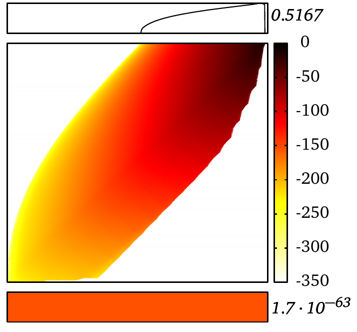
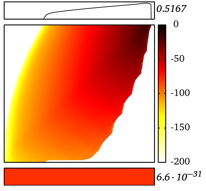
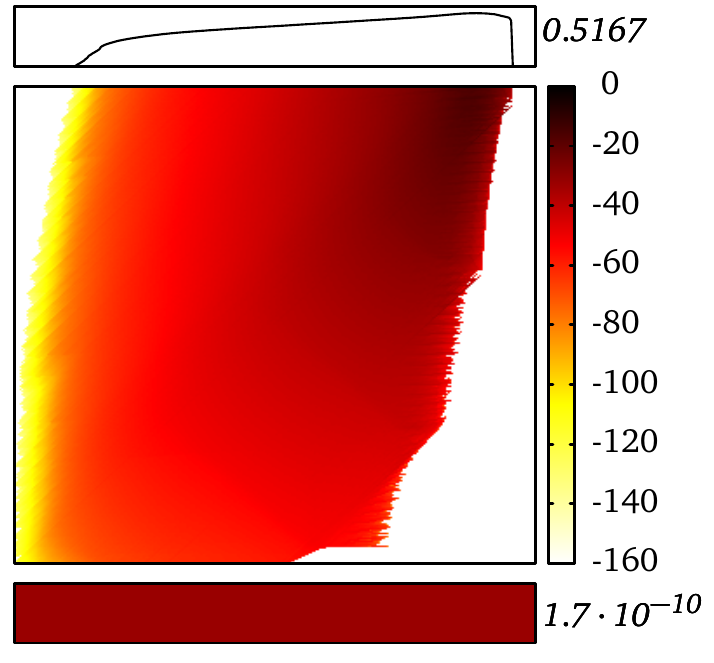
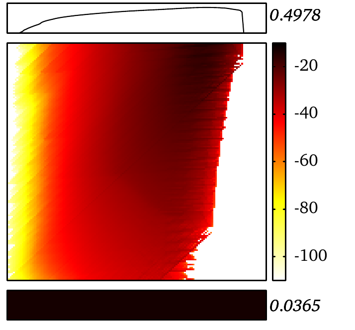
Figure 6: SoC of the satellite after $1$ year with different sizes of the battery. The leftmost SoC is with the original battery capacity, $5000$ mAh. In each further plot, the battery capacity is halved, i.e. $2500$ mAh, $1250$ mAh, and $625$ mAh. Note that all the densities are depicted on the logarithmic scale (numbers in the legend stand for the order of magnitude). We observe that only the smallest battery does not give sufficient guarantees. Its probability of depletion after $1$ year is $0.0365$; the probability gets down to $1.7\cdot 10^{-10}$ already for the $1250$ mAh battery. The smaller the battery, the more crucial is the distinction of available and bound charge as a larger area of the plots is filled with non-trivial density.

According to the above discussion, the load on the satellite is the superposition of two piecewise constant loads.

• A probabilistic load reflecting the different operation modes, modeled by a Markov task process $\mathcal{M}$as depicted in Figure 5.

• A strictly periodic charge load alternating between $66$ minutes at $-400$ mA, and the remaining $33$ minutes at $0$ mA.

One can easily express the charging load as another independent Markov task process (where all probabilities are $1$) and consider the sum load generated by these two processes in parallel (methods in Section 5 adapt straightforwardly to this setting).

The KiBaM in our model has following parameters:

• the ratio of the available charge $c=1/2$ (artificially chosen value as parameters fitted by experiments on similar batteries strongly vary [31, 20]);

• the diffusion rate $p=0.0006$ per minute (we decreased the value reported by experiments [20] by a factor of $4$ because of the low average temperature in orbit, $3.5^{\circ}$C, and the influence of the Arrhenius equation [23]).

Computational Aspects

We implemented the continuous solution developed in the previous sections in a high-level computational language Octave. This showed up to be practical only up to sequences of a handful of tasks. Therefore, we implemented a solution over a discretized abstraction of the stochastic process induced by the MTP and the battery. By fixing the number of discretization steps $K\in\mathbb{N}$ which yields the discretization step $\delta=\frac{d}{2}\cdot\frac{1}{K}$, we obtain battery states

• $\{(n,m)\mid 0<n<K,\;0<m<K\}$ in the inner space where each $(n,m)$ represents the adjacent rectangle of higher charge $[n\delta,(n+1)\delta)\times[m\delta,(m+1)\delta)$,

• states $\{(K,m)\mid 0<m<K\}$ on the capacity boundary where each $(K,m)$ represents the adjacent line of higher bound charge $\{\frac{d}{2}\}\times[m\delta,(m+1)\delta)$, and

• state $(0,0)$ for the rest, $\{(a,b)\mid\text{$a<\delta$ or $b<\delta$}\}$.

We always represent higher charge by lower charge (i.e. under-approximate SoC) since we are interested in guarantees on probabilities that the battery powers the MTP for a given time horizon. Similarly, we replace load distributions by discrete distributions where each point represents an adjacent left interval (i.e., we over-approximate the load). The continuous methods of Lemma 8 are easily adapted to this discrete setting, basically replacing integrals by finite sums.

This methods gives us an underapproximation of the probability that the battery powers the satellite. We do not have any prior error bound, but one can make the results arbitrarily precise by increasing $K$, at the price of quadratic cost increase.

Our implementation is done in C++, we used $K=$ 1200, 600, 300 and 150 for the experiments with the batteries of capacity $5000$ mAh, $2500$ mAh, $1250$ mAh and $625$ mAh, respectively to guarantee equal relative precision. All the experiments have been performed on a machine equipped with an Intel Core i5-2520M CPU @ 2.50GHz and 4GB RAM. All values occuring are represented and calculated with standard IEEE 754 double-precision binary floating-point format except for the values related to the battery being depleted where we use arbitrary precision arithmetic (as to this number, we keep adding values from the inner area that are of much lower order of magnitude).

Model evaluation

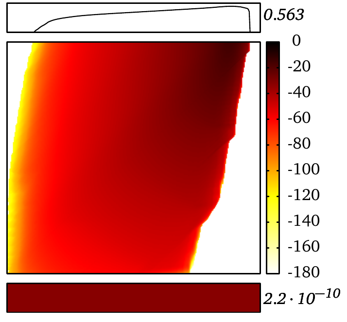
Figure 7: Load noise. The $1$ year run of the $1250$ mAh battery with Dirac loads on the left and with noisy loads on the right. We used Gaussian noise with standard deviation $5$.

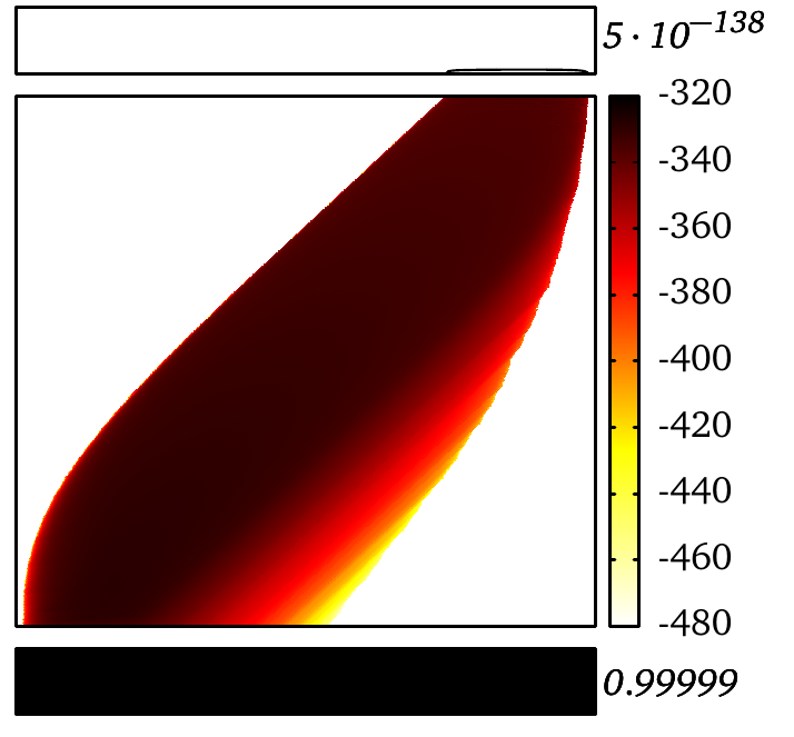
Figure 8: Number of solar panels. The full $5000$ mAh battery with $9$ solar panels on the left and $6$ solar panels on the right. This shows that for the current load, a $1$ unit cube design with solar panels on $6$ or less sides is not possible.

We performed various experiments with this model, to explore the random KiBaM technology. We here report on four distinct evaluations, demonstrating that valuable insight into the model can be obtained.

1. The $5000$ mAh battery in the real satellite is known to be over-dimensioned. Our aim was to find out how much. Hence, we performed a sequence of experiments, decreasing the size of the battery exponentially. The results are displayed and explained in Figure 1. We found out that $1/4$ of the capacity still provides sufficient guarantees to power the satellite for 1 year while $1/8$ of the capacity, $625$ mAh, does not.

2. We compared our results with a simple linear battery model of the same capacity. This linear model is not uncommon in the satellite domain, it has for instance been used in the Envisat and CryoSat missions [15]. We obtain the following probabilities for battery depletion:

   capacity	linear battery model	KiBaM
   5000 mAh	$1.86\cdot 10^{-84}$	$1.7\cdot 10^{-63}$
   625 mAh	$2.94\cdot 10^{-8}$	$0.0365$

   The linear model turns out to be surprisingly (and likely unjustifiably) optimistic, especially for the $625$ mAh battery.

3. We (computationally) simplified the two experiments above by assuming Dirac loads. To analyze the effect of the white noise, we compared the Dirac loads with the noisy loads, explained earlier, on the $625$ mAh battery. As expected, the noise (a) smoothes out the distribution a little and (b) pushes a bit more of the distribution to full and empty states, see Figure 7.

4. Our reference satellite is a two-unit satellite, i.e. is built from two cubes, each $10$ cm per side. In the current design, $9$ of the $10$ external sides are covered by solar panels, the remaining one is used for both radio antenna and camera. We thus analyzed whether a one-unit design with only $5$ solar panels is possible. The answer is negative, the system runs out of energy rapidly with high probability. Figure 8 displays that even for $6$ panels the charge level is highly insufficient to sustain the load.

7 Alternative Approaches

The results reported above are obtained from a discretized abstraction of the stochastic process induced by the MTP and the battery, solved numerically and with high-precision arithmetic where needed.

One could instead consider estimating the probability $z_{t}$ of the battery depletion using ordinary simulation techniques [16]. Considering a battery of capacity 5000 mAh, this would mean that about $10^{63}$ simulations traces are needed on average to observe the rare event of a depleted battery at least once. This seems prohibitive, also if resorting to massively parallel simulation, which may reduce the exponent by a small constant at most. A possible way out of this might lie in the use of rare event simulation techniques to speed up simulation [30].

The behaviour of KiBaM with capacity bounds can be expressed as a relatively simple hybrid automaton model [18]. Similarly, the random KiBaM with capacity bounds can be regarded as an instance of a stochastic hybrid system (SHS) [1, 2, 3, 6, 9, 28]. This observation opens some further evaluation avenues, since there are multiple tools available publicly for checking reachability properties of SHS. In particular, Faust² [11], SiSat [14] and ProHVer [32, 13] appear adequate at first sight. Our experiments with Faust² however were unsuccessful, basically due to a model mismatch: The tool thus far assumes stochasticity in all dimensions, because it operates on stochastic kernels, while our model is non-stochastic in the bound charge dimension. With SiSat, we so far failed to encode the MTP (or its effect) into an input accepted by the tool. The MTP can be considered as a compact description of an otherwise intricate semi-Markov process running on a discrete time line. This is in principle supported by SiSat, yet we effectively failed to provide a compact encoding. Our ProHVer experiments failed for a different reason, namely the sheer size of the problem. All the above tools have not been optimized for dealing with very low probabilities as they appear in the satellite case.

8 Conclusion

Inspired by the needs of an earth-orbiting satellite mission, we extended in this paper the theory of kinetic battery models in two independent dimensions. First, we addressed battery charging up to full capacity. Second, we extended the theory of the KiBaM differential equations to a stochastic setting. We provided a symbolic solution for random initial SoC and a sequence of piecewise-constant random loads.

These sequences can be generated by a stochastic process representing an abstract and averaged behavioral model of a nano satellite operating in earth orbit, superposed with a deterministic representation of the solar infeed in orbit. We illustrated the approach by several experiments performed on the model, especially varying the size of the battery, but also the number of solar panels.

ESA is running a large educational program [10] for launching missions akin to GOMX-1. The satellites are designed by student teams, have the form of standardized 1 unit cube with maximum mass of 1 kg, and target mission times of up to four years. The random KiBaM presented here is of obvious high relevance for any participating team. It can help quantify the risk of premature depletion for the various battery dimensions at hand, and thereby enable an optimal use of the available weight and space budget. Our experiments show that using the simpler linear battery model instead is far too optimistic in this respect.

For a fixed setup, one can also use the technology offered by us for optimal task scheduling: In the same way as we can follow a single SoC distribution, we can also branch into several distributions and determine which of them is best according to some metric. Taking inspiration from [31], this can be combined with statistical model checking so as to find the optimal task schedule of a given set of tasks.

Several extensions can and should be integrated in the model. Among them, temperature dependencies are of particular interest. A temperature change has namely opposing physical effects in solar panels and in the battery, having intriguing consequences such as piecewise exponential decay in the charging process. An extension that is particularly important for long lasting missions, is incorporating a model of battery wearout. So far we assume the battery capacity to be constant along the mission time. Notably, our contribution is the first to consider capacity bounds in operation at all, as far as we are aware.

Acknowledgements

The authors are grateful for inspiring discussions with Peter Bak (GomSpace ApS), Erik R. Wognsen (Aalborg University), and other members of the SENSATION consortium, as well as with Pascal Gilles (ESA Centre for Earth Observation), Xavier Bossoreille (Deutsches Zentrum für Luft- und Raumfahrt) and Marc Bouissou (Électricité de France S.A., École Centrale Paris - LGI). This work is supported by the Transregional Collaborative Research Centre SFB/TR 14 AVACS, and the 7th EU Framework Program under grant agreements 295261 (MEALS) and 318490 (SENSATION).

References

- [1] A. Abate, M. Prandini, J. Lygeros, and S. Sastry. Probabilistic reachability and safety for controlled discrete time stochastic hybrid systems. Automatica, 44(11):2724–2734, 2008.
- [2] E. Altman and V. Gaitsgory. Asymptotic optimization of a nonlinear hybrid system governed by a markov decision process. SIAM Journal on Control and Optimization, 35(6):2070–2085, 1997.
- [3] H. A. Blom, J. Lygeros, M. Everdij, S. Loizou, and K. Kyriakopoulos. Stochastic hybrid systems: theory and safety critical applications, volume 337. Springer Heidelberg, 2006.
- [4] U. Boker, T. A. Henzinger, and A. Radhakrishna. Battery transition systems. In Proceedings of the 41st annual ACM SIGPLAN-SIGACT symposium on Principles of programming languages, pages 595–606. ACM, 2014.
- [5] I. Buchmann. Batteries in a portable world. Cadex Electronics Richmond, 2001.
- [6] M. L. Bujorianu, J. Lygeros, and M. C. Bujorianu. Bisimulation for general stochastic hybrid systems. In Hybrid Systems: Computation and Control, pages 198–214. Springer, 2005.
- [7] L. Cloth, M. R. Jongerden, and B. R. Haverkort. Computing battery lifetime distributions. In The 37th Annual IEEE/IFIP International Conference on Dependable Systems and Networks, DSN 2007, 25-28 June 2007, Edinburgh, UK, Proceedings, pages 780–789. IEEE Computer Society, 2007.
- [8] R. M. Corless, G. H. Gonnet, D. E. G. Hare, D. J. Jeffrey, and D. E. Knuth. On the lambertW function. Adv. Comput. Math., 5(1):329–359, 1996.
- [9] M. H. Davis. Piecewise-deterministic markov processes: A general class of non-diffusion stochastic models. Journal of the Royal Statistical Society. Series B (Methodological), pages 353–388, 1984.
- [10] Esa. Esa cubesat program, Oct. 2014. http://www.esa.int/Education/CubeSats.
- [11] S. Esmaeil Zadeh Soudjani, C. Gevaerts, and A. Abate. Faust2: Formal abstractions of uncountable-state stochastic processes. arXiv preprint, 2014. arXiv:1403.3286.
- [12] M. Fox, D. Long, and D. Magazzeni. Automatic construction of efficient multiple battery usage policies. In T. Walsh, editor, IJCAI 2011, Proceedings of the 22nd International Joint Conference on Artificial Intelligence, Barcelona, Catalonia, Spain, July 16-22, 2011, pages 2620–2625. IJCAI/AAAI, 2011.
- [13] M. Fränzle, E. M. Hahn, H. Hermanns, N. Wolovick, and L. Zhang. Measurability and safety verification for stochastic hybrid systems. In HSCC, pages 43–52, New York, NY, USA, 2011. ACM Press.
- [14] M. Fränzle, H. Hermanns, and T. Teige. Stochastic satisfiability modulo theory: A novel technique for the analysis of probabilistic hybrid systems. In M. Egerstedt and B. Mishra, editors, Pre-Proceedings of the European Joint Conferences on Theory and Practice of Software (ETAPS) 2008 Sixth Workshop on Quantitative Aspects of Programming Languages (QAPL 2008), volume 4981 of Lecture Notes in Computer Science (LNCS), pages 172–186. Springer-Verlag, 2008. Extended abstract.
- [15] P. Gilles. Private communication. 2014.
- [16] D. T. Gillespie. A general method for numerically simulating the stochastic time evolution of coupled chemical reactions. Journal of computational physics, 22(4):403–434, 1976.
- [17] GomSpace. Gomspace gomx-1, Oct. 2014. http://gomspace.com/?p=gomx1.
- [18] T. A. Henzinger. The theory of hybrid automata. Springer, 2000.
- [19] M. Jongerden, B. Haverkort, H. Bohnenkamp, and J. Katoen. Maximizing system lifetime by battery scheduling. In Dependable Systems & Networks, 2009. DSN’09. IEEE/IFIP International Conference on, pages 63–72. IEEE, 2009.
- [20] M. R. Jongerden. Model-based energy analysis of battery powered systems. PhD thesis, Enschede, December 2010.
- [21] M. R. Jongerden and B. R. Haverkort. Which battery model to use? IET Software, 3(6):445–457, 2009.
- [22] E. A. Lee and D. G. Messerschmitt. Synchronous data flow. Proceedings of the IEEE, 75(9):1235–1245, 1987.
- [23] B. Y. Liaw, E. P. Roth, R. G. Jungst, G. Nagasubramanian, H. L. Case, and D. H. Doughty. Correlation of arrhenius behaviors in power and capacity fades with cell impedance and heat generation in cylindrical lithium-ion cells. Journal of power sources, 119:874–886, 2003.
- [24] J. F. Manwell and J. G. McGowan. Lead acid battery storage model for hybrid energy systems. Solar Energy, 50(5):399–405, 1993.
- [25] V. Rao, G. Singhal, A. Kumar, and N. Navet. Battery model for embedded systems. In 18th International Conference on VLSI Design (VLSI Design 2005), with the 4th International Conference on Embedded Systems Design, 3-7 January 2005, Kolkata, India, pages 105–110. IEEE Computer Society, 2005.
- [26] J. Rodríguez-Carvajal, G. Rousse, C. Masquelier, and M. Hervieu. Electronic crystallization in a lithium battery material: Columnar ordering of electrons and holes in the spinel . Phys. Rev. Lett., 81:4660–4663, Nov 1998.
- [27] R. A. Sahner and K. S. Trivedi. Performance and reliability analysis using directed acyclic graphs. IEEE Transactions on Software Engineering, 13(10):1105–1114, 1987.
- [28] J. Sproston. Decidable model checking of probabilistic hybrid automata. In Formal Techniques in Real-Time and Fault-Tolerant Systems, pages 31–45. Springer, 2000.
- [29] B. D. Theelen, M. Geilen, T. Basten, J. P. Voeten, S. V. Gheorghita, and S. Stuijk. A scenario-aware data flow model for combined long-run average and worst-case performance analysis. In Formal Methods and Models for Co-Design, 2006. MEMOCODE’06. Proceedings. Fourth ACM and IEEE International Conference on, pages 185–194. IEEE, 2006.
- [30] M. Villén-Altamirano and J. Villén-Altamirano. Restart: a straightforward method for fast simulation of rare events. In Simulation Conference Proceedings, 1994. Winter, pages 282–289. IEEE, 1994.
- [31] E. R. Wognsen, R. R. Hansen, and K. G. Larsen. Battery-aware scheduling of mixed criticality systems. In Leveraging Applications of Formal Methods, Verification and Validation. Specialized Techniques and Applications, pages 208–222. Springer Berlin Heidelberg, 2014.
- [32] L. Zhang, Z. She, S. Ratschan, H. Hermanns, and E. M. Hahn. Safety verification for probabilistic hybrid systems. In CAV, volume 6174 of LNCS, pages 196–211. Springer, 2010.