$\chi^{2}$-confidence sets in high-dimensional regression

Abstract

We study a high-dimensional regression model. Aim is to construct a confidence set for a given group of regression coefficients, treating all other regression coefficients as nuisance parameters. We apply a one-step procedure with the square-root Lasso as initial estimator and a multivariate square-root Lasso for constructing a surrogate Fisher information matrix. The multivariate square-root Lasso is based on nuclear norm loss with $\ell_{1}$-penalty. We show that this procedure leads to an asymptotically $\chi^{2}$-distributed pivot, with a remainder term depending only on the $\ell_{1}$-error of the initial estimator. We show that under $\ell_{1}$-sparsity conditions on the regression coefficients $\beta^{0}$ the square-root Lasso produces to a consistent estimator of the noise variance and we establish sharp oracle inequalities which show that the remainder term is small under further sparsity conditions on $\beta^{0}$ and compatibility conditions on the design.

1 Introduction

Let $X$ be a given $n\times p$ input matrix and $Y$ be a random $n$-vector of responses. We consider the high-dimensional situation where the number of variables $p$ exceeds the number of observations $n$. The expectation of $Y$ (assumed to exist) is denoted by $f^{0}:={\rm I\hskip-4.79996ptE}Y$. We assume that $X$ has rank $n$ ($n<p$) and let $\beta^{0}$ be any solution of the equation $X\beta^{0}=f^{0}$. Our aim is to construct a confidence interval for a pre-specified group of coefficients $\beta_{J}^{0}:=\{\beta_{j}^{0}:\ j\in J\}$ where $J\subset\{1,\ldots,p\}$ is a subset of the indices. In other words, the $|J|$-dimensional vector $\beta_{J}^{0}$ is the parameter of interest and all the other coefficients $\beta_{-J}^{0}:=\{\beta_{j}^{0}:\ j\notin J\}$ are nuisance parameters.

For one-dimensional parameters of interest ($|J|=1$) the approach in this paper is closely related to earlier work. The method is introduced in Zhang and Zhang (2014). Further references are Javanmard and Montanari (2013) and van de Geer et al. (2014). Related approaches can be found in Belloni et al. (2013a), Belloni et al. (2013b) and Belloni et al. (2014).

For confidence sets for groups of variables ($|J|>1$) one usually would like to take the dependence between estimators of single parameters into account. An important paper that carefully does this for confidence sets in $\ell_{2}$ is Mitra and Zhang (2014). Our approach is related but differs in an important way. As in Mitra and Zhang (2014) we propose a de-sparsified estimator which is (potentially) asymptotically linear. However, Mitra and Zhang (2014) focus at a remainder term which is small also for large groups. Our goal is rather to present a construction which has a small remainder term after studentizing and which does not rely on strong conditions on the design $X$. In particular we do not assume any sparsity conditions on the design.

The construction involves the square-root Lasso $\hat{\beta}$ which is introduced by Belloni et al. (2011). See Section 2 for the definition of the estimator $\hat{\beta}$. We present a a multivariate extension of the square-root Lasso which takes the nuclear norm of the multivariate residuals as loss function. Then we define in Section 3.1 a de-sparsified estimator $\hat{b}_{J}$ of $\beta_{J}^{0}$ which has the form of a one-step estimator with $\hat{\beta}_{J}$ as initial estimator and with multivariate square-root Lasso invoked to obtain a surrogate Fisher information matrix. We show that when $Y\sim{\cal N}_{n}(f^{0},\sigma_{0}^{2}I)$ (with both $f^{0}$ and $\sigma_{0}^{2}$ unknown), a studentized version of $\hat{b}_{J}-\beta_{J}^{0}$ has asymptotically a $|J|$-dimensional standard normal distribution.

More precisely we will show in Theorem 3.1 that for a given $|J|\times|J|$ matrix $M=M_{\lambda}$ depending only on $X$ and on a tuning parameter $\lambda$, one has $M_{\lambda}(\hat{b}_{J}-\beta_{J}^{0})/\sigma_{0}={\cal N}_{|J|}(0,I)+{\rm rem}$ where the remainder term “${\rm rem}$” can be bounded by $\|{\rm rem}\|_{\infty}\leq\sqrt{n}\lambda\|\hat{\beta}_{-J}-\beta_{-J}^{0}\|_{1}/\sigma_{0}$. The choice of the tuning parameter $\lambda$ is “free” (and not depending on $\sigma_{0}$), it can can for example be taken of order $\sqrt{\log p/n}$. The unknown parameter $\sigma_{0}^{2}$ can be estimated by the normalized residual sum of squares $\hat{\sigma}^{2}:=\|Y-X\hat{\beta}\|_{2}^{2}/n$ of the square-root Lasso $\hat{\beta}$. We show in Lemma 3 that under sparsity conditions on $\beta^{0}$ one has $\hat{\sigma}^{2}/\sigma_{0}^{2}=1+o_{{\rm I\hskip-1.54001ptP}}(1)$ and then in Theorem 4.1 an oracle inequality for the square-root Lasso under further sparsity conditions on $\beta^{0}$ and compatibility conditions on the design. The oracle result allows one to “verify” when $\sqrt{n}\lambda\|\hat{\beta}_{-J}-\beta_{-J}^{0}\|_{1}/\sigma_{0}=o_{{\rm I\hskip-1.54001ptP}}(1)$ so that the remainder term ${\rm rem}$ is negligible. An illustration assuming weak sparsity conditions is given in Section 5. As a consequence

$$\|M_{\lambda}(\hat{b}_{J}-\beta_{J}^{0})\|_{2}^{2}/\hat{\sigma}^{2}=\chi_{|J|}^{2}(1+o_{{\rm I\hskip-1.54001ptP}}(1)),$$

where $\chi_{|J|}^{2}$ is a random variable having a $\chi^{2}$-distribution with $|J|$ degrees of freedom. For $|J|$ fixed one can thus construct asymptotic confidence sets for $\beta_{J}^{0}$ (we will also consider the case $|J|\rightarrow\infty$ in Section 8). We however do not control the size of these sets. Larger values for $\lambda$ makes the confidence sets smaller but will also give a larger remainder term.

In Section 6 we extend the theory to structured sparsity norms other than $\ell_{1}$, for example the norm used for the (square-root) group Lasso, where the demand for $\ell_{2}$-confidence sets for groups comes up quite naturally. Section 8 contains a discussion. The proofs are in Section 9.

1.1 Notation

The mean vector of $Y$ is denoted by $f^{0}$ and the noise is $\epsilon:=Y-f^{0}$. For a vector $v\in\mathbb{R}^{n}$ we write (with a slight abuse of notation) $\|v\|_{n}^{2}:=v^{T}v/n$. We let $\sigma_{0}^{2}:={\rm I\hskip-4.79996ptE}\|\epsilon\|_{n}^{2}$ (assumed to exist).

For a vector $\beta\in\mathbb{R}^{p}$ we set $S_{\beta}:=\{j:\ \beta_{j}\not=0\}$. For a subset $J\subset\{1,\ldots,p\}$ and a vector $\beta\in\mathbb{R}^{p}$ we use the same notation $\beta_{J}$ for the $|J|$-dimensional vector $\{\beta_{j}:\ j\in J\}$ and the $p$-dimensional vector $\{\beta_{j,J}:=\beta_{j}{\rm l}\{j\in J\}:\ j=1,\ldots,p\}$. The last version allows us to write $\beta=\beta_{J}+\beta_{-J}$ with $\beta_{-J}=\beta_{J^{c}}$, $J^{c}$ being the complement of the set $J$. The $j$-th column of $X$ is denoted by $X_{j}$ ($j=1,\ldots,p$). We let $X_{J}:=\{X_{j}:\ j\in J\}$ and $X_{-J}:=\{X_{j}:\ j\notin J\}$.

For a matrix $A$ we let $\|A\|_{\rm nuclear}:={\rm trace}((A^{T}A)^{1/2})$ be its nuclear norm. The $\ell_{1}$-norm of the matrix $A$ is defined as $\|A\|_{1}:=\sum_{k}\sum_{j}|a_{k,j}|$. Its $\ell_{\infty}$-norm is $\|A\|_{\infty}:=\max_{k}\max_{j}|a_{k,j}|$.

2 The square-root Lasso and its multivariate version

2.1 The square-root Lasso

The square-root Lasso (Belloni et al. (2011)) $\hat{\beta}$ is

$$\hat{\beta}:=\arg\min_{\beta\in\mathbb{R}^{p}}\biggl{\{}\|Y-X\beta\|_{n}+\lambda_{0}\|\beta\|_{1}\biggr{\}}.$$ (1)

The parameter $\lambda_{0}>0$ is a tuning parameter. Thus $\hat{\beta}$ depends on $\lambda_{0}$ but we do not express this in our notation.

The square-root Lasso can be seen as a method that estimates $\beta^{0}$ and the noise variance $\sigma_{0}^{2}$ simultaneously. Defining the residuals $\hat{\epsilon}:=Y-X\hat{\beta}$ and letting $\hat{\sigma}^{2}:=\|\hat{\epsilon}\|_{n}^{2}$ one clearly has

$$(\hat{\beta},\hat{\sigma}^{2})=\arg\min_{\beta\in\mathbb{R}^{p},\ \sigma^{2}>0}\biggl{\{}{\|Y-X\beta\|_{n}^{2}\over\sigma}+\sigma+2\lambda_{0}\|\beta\|_{1}\biggr{\}}$$ (2)

provided the minimum is attained at a positive value of $\sigma^{2}$.

We note in passing that the square-root Lasso is not a quasi-likelihood estimator as the function $\exp[-z^{2}/\sigma-\sigma]$, $z\in\mathbb{R}$, is not a density with respect to a dominating measure not depending on $\sigma^{2}>0$. The square-root Lasso is moreover not to be confused with the scaled Lasso. The latter is a quasi-likelihood estimator. It is studied in e.g. Sun and Zhang (2012).

We show in Section 4.1 (Lemmas 2 and 3) that for the case where $\epsilon\sim{\cal N}_{n}(0,\sigma_{0}^{2}I)$ for example one has $\hat{\sigma}\rightarrow\sigma_{0}$ under $\ell_{1}$-sparsity conditions on $\beta^{0}$. In Section 4.2 we establish oracle results for $\hat{\beta}$ under further sparsity conditions on $\beta^{0}$ and compatibility conditions on $X$ (see Definition 2 for the latter). These results hold for a “universal” choice of $\lambda_{0}$ provided an $\ell_{1}$-sparsity condition on $\beta^{0}$ is met.

In the proof of our main result in Theorem 3.1, the so-called Karush-Kuhn-Tucker conditions, or KKT-conditions, play a major role. Let us briefly discuss these here. The KKT-conditions for the square-root Lasso say that

$${X^{T}(Y-X\hat{\beta})/n\over\hat{\sigma}}=\lambda_{0}\hat{z}$$ (3)

where $\hat{z}$ is a $p$-dimensional vector with $\|\hat{z}\|_{\infty}\leq 1$ and with $\hat{z}_{j}={\rm sign}(\hat{\beta}_{j})$ if $\hat{\beta}_{j}\not=0$. This follows from sub-differential calculus which defines the sub-differential of the absolute value function $x\mapsto|x|$ as

$$\{{\rm sign}(x)\}\{x\not=0\}+[-1,1]\{x=0\}.$$

Indeed, for a fixed $\sigma>0$ the sub-differential with respect to $\beta$ of the expression in curly brackets given in (2) is equal to

$$-{2X^{T}(Y-X\beta)/n\over\sigma}+2\lambda_{0}z(\beta)$$

with, for $j=1,\ldots,p$, $z_{j}(\beta)$ the sub-differential of $\beta_{j}\mapsto|\beta_{j}|$. Setting this to zero at $(\hat{\beta},\hat{\sigma})$ gives the above KKT-conditions (3).

2.2 The multivariate square-root Lasso

In our construction of confidence sets we will consider the regression of $X_{J}$ on $X_{-J}$ invoking a multivariate version of the square-root Lasso. To explain the latter, we use here a standard notation with $X$ being the input and $Y$ being the response. We will then replace $X$ by $X_{-J}$ and $Y$ by $X_{J}$ in Section 3.1.

The matrix $X$ is as before an $n\times p$ input matrix and the response $Y$ is now an $n\times q$ matrix for some $q\geq 1$. We define the multivariate square-root Lasso

$$\hat{B}:=\arg\min_{B}\biggr{\{}\|Y-XB\|_{\rm nuclear}/\sqrt{n}+\lambda_{0}\|B\|_{1}\biggr{\}}$$ (4)

with $\lambda_{0}>0$ again a tuning parameter. The minimization is over all $p\times q$ matrices $B$. We consider $\hat{\Sigma}:=(Y-X\hat{B})^{T}(Y-X\hat{B})/n$ as estimator of the noise co-variance matrix.

The KKT-conditions for the multivariate square-root Lasso will be a major ingredient of the proof of the main result in Theorem 3.1. We present these KKT-conditions in the following lemma in equation (5).

Lemma 1

We have

$$(\hat{B},\hat{\Sigma})=\arg\min_{B,\ \Sigma>0}\biggl{\{}{\rm trace}\biggl{(}(Y-XB)^{T}(Y-XB)\Sigma^{-1/2}\biggr{)}/n$$

$$\ \ \ \ \ \ \ \ \ \ \ \ \ \ \ \ +{\rm trace}(\Sigma^{1/2})+2\lambda_{0}\|B\|_{1}\biggr{\}}$$

where the minimization is over all symmetric positive definite matrix $\Sigma$ (this being denoted by $\Sigma>0$) and where it is assumed that the minimum is indeed attained at some $\Sigma>0$. The multivariate Lasso satisfies the KKT-conditions

$$X^{T}(Y-X\hat{B})\hat{\Sigma}^{-1/2}/n=\lambda_{0}\hat{Z},$$ (5)

where $\hat{Z}$ is a $p\times q$ matrix with $\|\hat{Z}\|_{\infty}\leq 1$ and with $\hat{Z}_{k,j}={\rm sign}(\hat{B}_{k,j})$ if $\hat{B}_{k,j}\not=0$ ($k=1,\ldots,p$, $j=1,\ldots,q$).

3 Confidence sets for $\beta_{J}^{0}$

3.1 The construction

Let $J\subset\{1,\ldots,p\}$. We are interested in building a confidence set for $\beta_{J}^{0}:=\{\beta_{j}^{0}:\ j\in J\}$. To this end, we compute the multivariate ($|J|$-dimensional) square root Lasso

$$\hat{\Gamma}_{J}:=\arg\min_{\Gamma_{J}}\biggl{\{}\|X_{J}-X_{-J}\Gamma_{J}\|_{\rm nuclear}/\sqrt{n}+\lambda\|\Gamma_{J}\|_{1}\biggr{\}}$$ (6)

where $\lambda>0$ is a tuning parameter. The minimization is over all $(p-|J|)\times|J|$ matrices $\Gamma_{J}$. We let

$$\tilde{T}_{J}:=(X_{J}-X_{-J}\hat{\Gamma}_{J})^{T}X_{J}/n$$ (7)

and

$$\hat{T}_{J}:=(X_{J}-X_{-J}\hat{\Gamma}_{J})^{T}(X_{J}-X_{-J}\hat{\Gamma}_{J})/n,$$ (8)

We assume throughout that the “hat” matrix $\hat{T}_{J}$ is non-singular. The “tilde” matrix $\tilde{T}_{J}$ only needs to be non-singular in order that the de-sparsified estimator $\hat{b}_{J}$ given below in Definition 1 is well-defined. However, for the normalized version we need not assume non-singularity of $\tilde{T}_{J}$.

The KKT-conditions (5) appear in the form

$$X_{-J}^{T}(X_{J}-X_{-J}\hat{\Gamma}_{J})\hat{T}_{J}^{-1/2}/n=\lambda\hat{Z}_{J},$$ (9)

where $\hat{Z}_{J}$ is a $(p-|J|)\times|J|$ matrix with $(\hat{Z}_{J})_{k,j}={\rm sign}(\hat{\Gamma}_{J})_{k,j}$ if $(\hat{\Gamma}_{J})_{k,j}\not=0$ and $\|\hat{Z}_{J}\|_{\infty}\leq 1$.

We define the normalization matrix

$$M:=M_{\lambda}:=\sqrt{n}\hat{T}_{J}^{-1/2}\tilde{T}_{J}.$$ (10)

Definition 1

The de-sparsified estimator of $\beta_{J}^{0}$ is

$$\hat{b}_{J}:=\hat{\beta}_{J}+\tilde{T}_{J}^{-1}(X_{J}-X_{-J}\hat{\Gamma}_{J})^{T}(Y-X\hat{\beta})/n,$$

with $\hat{\beta}$ the square-root Lasso given in (1), $\hat{\Gamma}_{J}$ the multivariate square-root Lasso given in (6) and the matrix $\tilde{T}_{J}$ given in (7). The normalized de-sparsified estimator is $M\hat{b}_{J}$ with $M$ the normalization matrix given in (10).

3.2 The main result

Our main result is rather simple. It shows that using the multivariate square-root Lasso for de-sparsifying, and then normalizing, results in a well-scaled “asymptotic pivot” (up to the estimation of $\sigma_{0}$ which we will do in the next section). Theorem 3.1 actually does not require $\hat{\beta}$ to be the square-root Lasso but for definiteness we have made this specific choice throughout the paper (except for Section 6).

Theorem 3.1

Consider the model $Y\sim{\cal N}_{n}(f^{0},\sigma_{0}^{2})$ where $f^{0}=X\beta^{0}$. Let $\hat{b}_{J}$ be the de-sparsified estimator given in Definition 1 and let $M\hat{b}_{J}$ be its normalized version. Then

$$M(\hat{b}_{J}-\beta_{J}^{0})/\sigma_{0}={\cal N}_{|J|}(0,I)+{\rm rem}$$

where $\|{\rm rem}\|_{\infty}\leq\sqrt{n}\lambda\|\hat{\beta}_{-J}-\beta_{-J}^{0}\|_{1}/\sigma_{0}$.

To make Theorem 3.1 work we need to bound $\|\hat{\beta}-\beta^{0}\|_{1}/\hat{\sigma}$ where $\hat{\sigma}$ is an estimator of $\sigma_{0}$. This is done in Theorem 4.1 with $\hat{\sigma}$ the estimator $\|\hat{\epsilon}\|_{n}$ from the square-root Lasso. A special case is presented in Lemma 5 which imposes weak sparsity conditions for $\beta^{0}$. Bounds for $\sigma_{0}/\hat{\sigma}$ are also given.

Theorem 3.1 is about the case where the noise $\epsilon$ is i.i.d. normally distributed. This can be generalized as from the proof we see that the “main” term is linear in $\epsilon$. For independent errors with common variance $\sigma_{0}^{2}$ say, one needs to assume the Lindeberg condition for establishing asymptotic normality.

4 Theory for the square root Lasso

Let $f^{0}:={\rm I\hskip-4.79996ptE}Y$, $\beta^{0}$ be a solution of $X\beta^{0}=f^{0}$ and define $\epsilon:=Y-f^{0}$. Recall the square-root Lasso $\hat{\beta}$ given in (1). It depends on the tuning parameter $\lambda_{0}>0$. In this section we develop theoretical bounds, which are closely related to results in Sun and Zhang (2013) (who by the way use the term scaled Lasso instead of square-root Lasso in that paper). There are two differences. Firstly, our lower bound for the residual sum of squares of the square-root Lasso requires, for the case where no conditions are imposed on the compatibility constants, a smaller value for the tuning parameter (see Lemma 3). These compatibility constants, given in Definition 2, are required only later for the oracle results. Secondly, we establish an oracle inequality that is sharp (see Theorem 4.1 in Section 4.2 where we present more details).

Write $\hat{\epsilon}:=Y-X\hat{\beta}$ and $\hat{\sigma}^{2}:=\|\hat{\epsilon}\|_{n}^{2}$. We consider bounds in terms of $\|\epsilon\|_{n}^{2}$, the “empirical” variance of the unobservable noise. This is a random quantity but under obvious conditions it convergences to its expectation $\sigma_{0}^{2}$. Another random quantity that appears in our bounds is $\epsilon/\|\epsilon\|_{n}$, which is a random point on the $n$-dimensional unit sphere. We write

$$\hat{R}:={\|X^{T}\epsilon\|_{\infty}\over n\|\epsilon\|_{n}}.$$

When all $X_{j}$ are normalized such that $\|X_{j}\|_{n}=1$, the quantity $\hat{R}$ is the maximal “empirical” correlation between noise and input variables. Under distributional assumptions $\hat{R}$ can be bounded with large probability by some constant $R$. For completeness we work out the case of i.i.d. normally distributed errors.

Lemma 2

Let $\epsilon\sim{\cal N}_{n}(0,\sigma_{0}^{2}I)$. Suppose the normalized case where $\|X_{j}\|_{n}=1$ for all $j=1,\ldots,p$. Let $\alpha_{0}$, $\underline{\alpha}$ and $\bar{\alpha}$ be given positive error levels such that $\alpha_{0}+\underline{\alpha}+\bar{\alpha}<1$ and $\log(1/{\underline{\alpha}})<n/4$. Define

$${\underline{\sigma}}^{2}:=\sigma_{0}^{2}\biggl{(}1-2\sqrt{\log(1/{\underline{\alpha}})\over n}\biggr{)},$$

$${\bar{\sigma}}^{2}:=\sigma_{0}^{2}\biggl{(}1+2\sqrt{\log(1/{\bar{\alpha}})\over n}+{2\log(1/{\bar{\alpha}})\over n}\biggr{)}$$

and

$$R:=\sqrt{\log(2p/\alpha_{0})\over n-2\sqrt{n\log(1/{\underline{\alpha}})}}.$$

We have

$${\rm I\hskip-2.20001ptP}(\|\epsilon\|_{n}\leq{\underline{\sigma}})\leq{\underline{\alpha}},\ {\rm I\hskip-2.20001ptP}(\|\epsilon\|_{n}\geq\bar{\sigma})\leq\bar{\alpha}$$

and

$${\rm I\hskip-2.20001ptP}(\hat{R}\geq R\ \cup\|\epsilon\|_{n}\leq{\underline{\sigma}})\leq\alpha_{0}+{\underline{\alpha}}.$$

4.1 Preliminary lower and upper bounds for $\hat{\sigma}^{2}$

We now show that the estimator of the variance $\hat{\sigma}^{2}=\|\hat{\epsilon}\|_{n}^{2}$, obtained by applying the square-root Lasso, converges to the noise variance $\sigma_{0}^{2}$. The result holds without conditions on compatibility constants (given in Definition 2). We do however need the $\ell_{1}$-sparsity condition (11) on $\beta_{0}$. This condition will be discussed below in an asymptotic setup.

Lemma 3

Suppose that for some $0<\eta<1$, some $R>0$ and some ${\underline{\sigma}}>0$, we have

$$\lambda_{0}(1-\eta)\geq R$$

and

$$\lambda_{0}\|\beta^{0}\|_{1}/{\underline{\sigma}}\leq 2\biggl{(}\sqrt{1+(\eta/2)^{2}}-1\biggr{)}.$$ (11)

Then on the set where $\hat{R}\leq R$ and $\|\epsilon\|_{n}\geq{\underline{\sigma}}$ we have $\biggl{|}\|\hat{\epsilon}\|_{n}/\|\epsilon\|_{n}-1\biggr{|}\leq\eta$.

We remark here that the the result of Lemma 3 is also useful when using a square-root Lasso for constructing an asymptotic confidence interval for a single parameter, say $\beta_{j}^{0}$. Assuming random design it can be applied to show that without imposing compatibility conditions the residual variance of the square root Lasso for the regression of $X_{j}$ on all other variables $X_{-j}$ does not degenerate.

Asymptotics Suppose $\epsilon_{1},\ldots,\epsilon_{n}$ are i.i.d. with finite variance $\sigma_{0}^{2}$. Then clearly $\|\epsilon\|_{n}/\sigma_{0}\rightarrow 1$ in probability. The normalization in (11) by $\underline{\sigma}$ - which can be taken more or less equal to $\sigma_{0}$ - makes sense if we think of the standardized model

$$\tilde{Y}=X\tilde{\beta}^{0}+\tilde{\epsilon},$$

with $\tilde{Y}=Y/\sigma_{0}$, $\tilde{\beta}^{0}=\beta^{0}/\sigma_{0}$ and $\tilde{\epsilon}=\epsilon/\sigma_{0}$. The condition (11) is a condition on the normalized $\tilde{\beta}^{0}$. The rate of growth assumed there is quite common. First of all, it is clear that if $\|\beta^{0}\|_{1}$ is very large then the estimator is not very good because of the penalty on large values of $\|\cdot\|_{1}$. The condition (11) is moreover closely related to standard assumptions in compressed sensing. To explain this we first note that

$$\|\beta^{0}\|_{1}/\sigma_{0}\leq\sqrt{s_{0}}\|\beta^{0}\|_{2}/\sigma_{0}$$

when $s_{0}$ is the number of non-zero entries of $\beta^{0}$ (observe that $s_{0}$ is a scale free property of $\beta^{0}$). The term $\|\beta^{0}\|_{2}/\sigma_{0}$ can be seen as a signal-to-noise ratio. Let us assume this signal-to-noise ratio stays bounded. If $\lambda_{0}$ corresponds to the standard choice $\lambda_{0}\asymp\sqrt{\log p/n}$ the assumption (11) holds with $\eta=o(1)$ as soon as we assume the standard assumption $s_{0}=o(n/\log p)$.

4.2 An oracle inequality for the square-root Lasso

Our next result is an oracle inequality for the square-root Lasso. It is as the corresponding result for the Lasso as established in Bickel et al. (2009). The oracle inequality of Theorem 4.1 is sharp in the sense that there is a constant 1 in front of the approximation error $\|X(\beta-\beta^{0})\|_{n}^{2}$ in (12). This sharpness is obtained along the lines of arguments from Koltchinskii et al. (2011), who prove sharp oracle inequalities for the Lasso and for matrix problems. We further have extended the situation in order to establish an oracle inequality for the $\ell_{1}$-estimation error $\|\hat{\beta}-\beta^{0}\|_{1}$ where we use arguments from van de Geer (2014) for the Lasso. For the square-root Lasso, the paper Sun and Zhang (2013) also has oracle inequalities, but these are not sharp.

Compatibility constants are introduced in van de Geer (2007). They play a role in the identifiability of $\beta^{0}$.

Definition 2

Let $L>0$ and $S\subset\{1,\ldots,p\}$. The compatibility constant is

$$\hat{\phi}^{2}(L,S)=\min\biggl{\{}|S|\|X\beta\|_{n}^{2}:\ \|\beta_{S}\|_{1}=1,\ \|\beta_{-S}\|_{1}\leq L\biggr{\}}.$$

We recall the notation $S_{\beta}=\{j:\ \beta_{j}\not=0\}$ appearing in (12).

Theorem 4.1

Let $\lambda_{0}$ satisfy for some $R>0$

$$\lambda_{0}(1-\eta)>R$$

and assume the $\ell_{1}$-sparsity (11) for some $0<\eta<1$ and $\underline{\sigma}>0$, i.e.

$$\lambda_{0}\|\beta^{0}\|_{1}/{\underline{\sigma}}\leq 2\biggl{(}\sqrt{1+(\eta/2)^{2}}-1\biggr{)}.$$

Let $0\leq\delta<1$ be arbitrary and define

$$\underline{\lambda}:=\lambda_{0}(1-\eta)-R,$$

$$\bar{\lambda}:=\lambda_{0}(1+\eta)+R+\delta\underline{\lambda}$$

and

$$L:={\bar{\lambda}\over(1-\delta)\underline{\lambda}}.$$

Then on the set where $\hat{R}\leq R$ and $\|\epsilon\|_{n}\geq{\underline{\sigma}}$, we have

$$2\delta\underline{\lambda}\|\hat{\beta}-\beta^{0}\|_{1}\|\epsilon\|_{n}+\|X(\hat{\beta}-\beta^{0})\|_{n}^{2}$$

$$\leq\min_{S}\biggl{\{}\min_{\beta\in\mathbb{R}^{p},\ S_{\beta}=S}\biggl{[}2\delta\underline{\lambda}\|\beta-\beta^{0}\|_{1}\|\epsilon\|_{n}+\|X(\beta-\beta^{0})\|_{n}^{2}\biggr{]}+{\bar{\lambda}}^{2}{|S|\|\epsilon\|_{n}^{2}\over\hat{\phi}^{2}(L,S)}\biggr{\}}.$$ (12)

The result of Theorem 4.1 leads to a trade-off between the approximation error $\|X(\beta-\beta^{0})\|_{n}^{2}$, the $\ell_{1}$-error $\|\beta-\beta^{0}\|_{1}$ and the sparseness $|S_{\beta}|$ (or rather the effective sparseness $|S_{\beta}|/\hat{\phi}^{2}(L,S_{\beta})$).

5 A bound for the $\ell_{1}$-estimation error under (weak) sparsity

In this section we assume

$$\sum_{j=1}^{r}|\beta_{j}^{0}|^{r}\leq\rho_{r}^{r},$$ (13)

where $0<r<1$ and where $\rho_{r}>0$ is a constant that is “not too large”. This is sometimes called weak sparsity as opposed to strong sparsity which requires ”not too many” non-zero coefficients $s_{0}:=\#\{\beta_{j}^{0}\not=0\}$. We start with bounding the right hand side of the oracle inequality (12) in Theorem 4.1.

We let $S_{0}:=S_{\beta^{0}}$ be the active set $S_{0}:=\{j:\beta_{j}^{0}\not=0\}$ of $\beta_{0}$ and let $\hat{\Lambda}_{\rm max}^{2}(S_{0})$ be the largest eigenvalue of $X_{S_{0}}^{T}X_{S_{0}}/n$. The cardinality of $S_{0}$ is denoted by $s_{0}=|S_{0}|$. We assume in this section the normalization $\|X_{j}\|_{n}=1$ so that that $\hat{\Lambda}_{\rm max}(S_{0})\geq 1$ and ans $\hat{\phi}(L,S)\leq 1$ for any $L$ and $S$.

Lemma 4

Suppose $\beta^{0}$ satisfies the weak sparsity condition (13) for some $0<r<1$ and $\rho_{r}>0$. For any positive $\delta$, ${\underline{\lambda}}$, $\bar{\lambda}$ and $L$

$$\min_{S}\biggl{\{}\min_{\beta\in\mathbb{R}^{p},\ S_{\beta}=S}\biggl{[}2\delta\underline{\lambda}\|\beta-\beta^{0}\|_{1}\|\epsilon\|_{n}+\|X(\beta-\beta^{0})\|_{n}^{2}\biggr{]}+{\bar{\lambda}}^{2}{|S|\|\epsilon\|_{n}^{2}\over\hat{\phi}^{2}(L,S)}\biggr{\}}$$

$$\leq 2{\bar{\lambda}}^{2-r}\biggl{(}\delta{\underline{\lambda}}/\bar{\lambda}+{\hat{\Lambda}_{\rm max}^{r}(S_{0})\over\hat{\phi}^{2}(L,\hat{S}_{*})}\biggr{)}\biggr{(}{\rho_{r}\over\|\epsilon\|_{n}}\biggr{)}^{r}\|\epsilon\|_{n}^{2},$$

where ${\hat{S}_{*}}:=\{j:\ |\beta_{j}^{0}|>\bar{\lambda}\|\epsilon\|_{n}/\hat{\Lambda}_{\rm max}(S_{0})\}$.

As a consequence, we obtain bounds for the prediction error and $\ell_{1}$-error of the square-root Lasso under (weak) sparsity. We only present the bound for the $\ell_{1}$-error as this is what we need in Theorem 3.1 for the construction of asymptotic confidence sets.

To avoid being taken away by all the constants, we make some arbitrary choices in Lemma 5: we set $\eta\leq 1/3$ in the $\ell_{1}$-sparsity condition (11) and we set $\lambda_{0}(1-\eta)=2R$. We choose $\delta=1/7$.

We include the confidence statements that are given in Lemma 2 to complete the picture.

Lemma 5

Suppose $\epsilon\sim{\cal N}_{n}(0,\sigma_{0}^{2}I)$. Let $\alpha_{0}$ and $\underline{\alpha}$ be given positive error levels such that $\alpha_{0}+\underline{\alpha}<1$ and $\log(1/{\underline{\alpha}})<n/4$. Define

$${\underline{\sigma}}^{2}:=\sigma_{0}^{2}\biggl{(}1-2\sqrt{\log(1/{\underline{\alpha}})\over n}\biggr{)},\ R:=\sqrt{\log(2p/\alpha_{0})\over n-2\sqrt{n\log(1/{\underline{\alpha}})}}.$$

Assume the $\ell_{1}$-sparsity condition

$$R\|\beta^{0}\|_{1}/{\underline{\sigma}}\leq(1-\eta)\biggl{(}\sqrt{1+(\eta/2)^{2}}-1\biggr{)},\ where\ 0<\eta\leq 1/3$$

and the $\ell_{r}$-sparsity condition (13) for some $0<r<1$ and $\rho_{r}>0$. Set

$${S_{*}}:=\{j:\ |\beta_{j}^{0}|>3R\underline{\sigma}/\hat{\Lambda}_{\rm max}(S_{0})\}.$$

Then for $\lambda_{0}(1-\eta)=2R$, with probability at least $1-\alpha_{0}-{\underline{\alpha}}$ we have the $\ell_{r}$-sparsity based bound

$$(1-\eta){\|\hat{\beta}-\beta^{0}\|_{1}\over\hat{\sigma}}\leq{\|\hat{\beta}-\beta^{0}\|_{1}\over\|\epsilon\|_{n}}\leq{(6R)}^{1-r}\biggl{(}1+{6^{2}\hat{\Lambda}_{\rm max}^{r}(S_{0})\over\hat{\phi}^{2}(6,S_{*})}\biggr{)}\biggr{(}{\rho_{r}\over{\underline{\sigma}}}\biggr{)}^{r},$$

the $\ell_{0}$-sparsity based bound

$$(1-\eta){\|\hat{\beta}-\beta^{0}\|_{1}\over\hat{\sigma}}\leq{\|\hat{\beta}-\beta^{0}\|_{1}\over\|\epsilon\|_{n}}\leq 3R\biggl{(}{6^{2}s_{0}\over\hat{\phi}^{2}(6,S_{0})}\biggr{)}$$

and moreover the following lower bound for the estimator $\hat{\sigma}$ of the noise level:

$$(1-\eta)\sigma_{0}/\hat{\sigma}\leq\biggl{(}1-2\sqrt{\log(1/{\underline{\alpha}})\over n}\biggr{)}^{-1/2}.$$

Asymptotics Application of Theorem 3.1 with $\sigma_{0}$ estimated by $\hat{\sigma}$ requires that $\sqrt{n}\lambda\|\hat{\beta}-\beta^{0}\|_{1}/\hat{\sigma}$ tends to zero in probability. Taking $\lambda\asymp\sqrt{\log p/n}$ and for example $\alpha_{0}=\alpha=1/p$, we see that this is the case under the conditions of Lemma 5 as soon as for some $0<r<1$ the following $\ell_{r}$-sparsity based bound holds:

$$\biggl{(}{\hat{\Lambda}_{\rm max}^{r}(S_{0})\over\hat{\phi}^{2}(6,S_{*})}\biggr{)}\biggl{(}{\rho_{r}\over\sigma_{0}}\biggr{)}^{r}={o(n/\log p)^{1-r\over 2}\over{(\log p)^{1\over 2}}}.$$

Alternatively, one may require the $\ell_{0}$-sparsity based bound

$$\biggl{(}{1\over\hat{\phi}^{2}(6,S_{0})}\biggr{)}{s_{0}}={o(n/\log p)^{1\over 2}\over(\log p)^{1\over 2}}.$$

6 Structured sparsity

We will now show that the results hold for norm-penalized estimators with norms other than $\ell_{1}$. Let $\Omega$ be some norm on $\mathbb{R}^{p-|J|}$ and define for a $(p-|J|)\times|J|$ matrix $A:=(a_{1},\ldots,a_{|J|})$

$$\|A\|_{1,\Omega}:=\sum_{j=1}^{|J|}\Omega(a_{j}).$$

For a vector $z\in\mathbb{R}^{p-|J|}$ we define the dual norm

$$\Omega_{*}(z)=\sup_{\Omega(a)\leq 1}|z^{T}a|,$$

and for a $(p-|J|)\times|J|$ matrix $Z=(z_{1},\ldots,z_{|J|})$ we let

$$\|Z\|_{\infty,\Omega_{*}}=\max_{1\leq j\leq|J|}\Omega_{*}(z_{j}).$$

Thus, when $\Omega$ is the $\ell_{1}$-norm we have $\|A\|_{1,\Omega}=\|A\|_{1}$ and $\|Z\|_{\infty,\Omega_{*}}=\|Z\|_{\infty}$. We let the multivariate square-root $\Omega$-sparse estimator be

$$\hat{\Gamma}_{J}:=\arg\min_{\Gamma_{J}}\biggl{\{}\|X_{J}-X_{-J}\Gamma_{J}\|_{\rm nuclear}/\sqrt{n}+\lambda\|\Gamma\|_{1,\Omega}\biggr{\}}.$$

This estimator equals (6) when $\Omega$ is the $\ell_{1}$-norm.

We let, as in (7), (8) and (10) but now with the new $\hat{\Gamma}_{J}$, the quantities $\tilde{T}_{J}$, $\hat{T}_{J}$ and $M$ be defined as

$$\tilde{T}_{J}:=(X_{J}-X_{-J}\hat{\Gamma}_{J})^{T}X_{J}/n,$$

$$\hat{T}_{J}:=(X_{J}-X_{-J}\hat{\Gamma}_{J})^{T}(X_{J}-X_{-J}\hat{\Gamma}_{J})/n$$

and

$$M:=M_{\lambda}:=\sqrt{n}\hat{T}_{J}^{-1/2}\tilde{T}_{J}.$$

The $\Omega$-de-sparsified estimator of $\beta_{J}^{0}$ is as in Definition 1

$$\hat{b}_{J}:=\hat{\beta}_{J}+\tilde{T}_{J}^{-1}(X_{J}-X_{-J}\hat{\Gamma}_{J})^{T}(Y-X\hat{\beta})/n,$$

but now with $\hat{\beta}$ not necessarily the square root Lasso but a suitably chosen initial estimator and with $\hat{\Gamma}_{J}$ the multivariate square-root $\Omega$-sparse estimator. The normalized de-sparsified estimator is $M\hat{b}_{J}$ with normalization matrix $M$ given above. We can then easily derive the following extension of Theorem 3.1.

Theorem 6.1

Consider the model $Y\sim{\cal N}_{n}(f^{0},\sigma_{0}^{2})$ where $f^{0}=X\beta^{0}$. Let $\hat{b}_{J}$ be the $\Omega$-de-sparsified estimator depending on some initial estimator $\hat{\beta}$. Let $M\hat{b}_{J}$ be its normalized version. Then

$$M(\hat{b}_{J}-\beta_{J}^{0})/\sigma_{0}={\cal N}_{|J|}(0,I)+{\rm rem}$$

where $\|{\rm rem}\|_{\infty}\leq\sqrt{n}\lambda\Omega(\hat{\beta}_{-J}-\beta_{-J}^{0})/\sigma_{0}$.

We see from Theorem 6.1 that confidence sets follow from fast rates of convergence of the $\Omega$-estimation error. The latter is studied in Bach (2010), Obozinski and Bach (2012) and van de Geer (2014) for the case where the initial estimator is the least squares estimator with penalty based on a sparsity inducing norm $\bar{\Omega}$ (say). Group sparsity Yuan and Lin (2006) is an example which we shall now briefly discuss.

Example 1

Let $G_{1},\ldots,G_{T}$ be given mutually disjoint subsets of $\{1,\ldots,p\}$ and take as sparsity-inducing norm

$$\bar{\Omega}(\beta):=\sum_{t=1}^{T}\sqrt{|G_{t}|}\|X\beta_{G_{t}}\|_{2},\ \beta\in\mathbb{R}^{p}.$$

The group Lasso is the minimizer of least squares loss with penalty proportional to $\bar{\Omega}$. Oracle inequalities for the $\bar{\Omega}$-error of the group Lasso have been derived in Lounici et al. (2011) for example. For the square-root version we refer to Bunea et al. (2013). With group sparsity, it lies at hand to consider confidence sets for one of the groups $G_{t}$ i.e., to take $J=G_{t_{0}}$ for a given $t_{0}$. Choosing

$$\Omega(a)=\sum_{t\not=t_{0}}\sqrt{|G_{t}|}\|Xa_{G_{t}}\|_{2},\ a\in\mathbb{R}^{p-|G_{t_{0}}|}$$

will ensure that $\Omega(\hat{\beta}_{-G_{t_{0}}}-\beta_{-G_{t_{0}}})\leq\bar{\Omega}(\hat{\beta}-\beta^{0})$ which gives one a handle to control the remainder term in Theorem 6.1. This choice of $\Omega$ for constructing the confidence set makes sense if one believes that the group structure describing the relation between the response $Y$ and the input $X$ is also present in the relation between $X_{G_{t_{0}}}$ and $X_{-G_{t_{0}}}$.

7 Simulations

Here we denote by $\widetilde{Y}=\widetilde{X}B_{0}+\epsilon$ an arbitrary linear multivariate regression. In a similar fashion to the suqare-root Algorithm in Buena et al. (2014) we propose the following algorithm for the multivariate square-root Lasso:

Algorithm 1 msrL

1:Take a constant $K$ big enough, and choose an arbitrary starting matrix $B(0)\in\mathbb{R}^{p\times q}$.

2:$\widetilde{Y}\leftarrow\widetilde{Y}/K$

3:$\widetilde{X}\leftarrow\widetilde{X}/K$

4:for $t=0,1,2,...t_{stop}$ do

5:     $B(t+1):=\overline{\Phi}\left(B(t)+X^{T}\cdot(Y-XB(t));\text{ }\lambda\|Y-XB(t)\|_{nuclear}\right)$

6:return $B(t_{stop}+1)$

Here we denote

$$\overline{\Phi}(a;\eta):=\begin{cases}0,&\mbox{if }a=0\\ \frac{a}{\|a\|_{2}}(\|a\|_{2}-\eta)_{+},&\mbox{if }a>0\end{cases}.$$

The value $t_{stop}$ can be chosen in such a way that one gets the desired accuracy for the algorithm. This algorithm is based on a Fixpoint equation from the KKT conditions. The square root Lasso is calculated via the algorithm in Buena et al. (2014).

We consider the usual linear regression model:

$$Y=X\beta+\epsilon.$$

In our simulations we take a design matrix X, where the rows are fixed i.i.d. realizations from $\mathcal{N}(0,\Sigma)$. We have $n$ observations, and $p$ explanatory variables. The covariance matrix $\Sigma$ has the following toeplitz structure $\Sigma_{i,j}=0.9^{|i-j|}$. The errors are i.i.d. Gaussian distributied, with variance $\sigma^{2}=1$. A set of points $J$ is also chosen. $J$ denotes the set of indices of the parameter vector $\beta$ that we want to find asymptotic group confidence intervals for. Define as $q=|J|$ the number of indices of interest. For each different setting of $p$ and $n$ we do $r=1000$ simulations. In each repetition we calculate the teststatistic $\chi^{2}$. A significance level of $0.05$ is chosen. The lambda of the square root LASSO $\lambda_{srL}$ in the simulations is the theoretical lambda $\lambda_{srLt}$ scaled by $3$. For the lambda of the multivariate square root LASSO $\lambda_{msrL}$ we do not have theoretical results yet. That is why we use cross-validation where we minimize the error expressed in nuclear norm, to define $\lambda_{msrL}$. It is important to note, that the choice of $\lambda_{msrL}$ is very crucial, especially for cases where $n$ is small. One could tune $\lambda_{msrL}$ in such a fashion that even cases like $n=100$ work much better, see figure 2. But the point here is to see what happens to the chi-squared test statistic with a fixed rule for the choice of $\lambda_{msrL}$. This basic set up is used throughout all the simulations below.

7.1 Asymptotic distribution

First let us look at the question how the histogram of the teststatistic looks like for different $n$. Here we use $p=500$ and $q=6$ with $J=(1,3,4,8,10,33)$, where the entries in $\beta_{J}$ are chosen randomly from a Uniform distribution on $[1,4]$. We also specify $\beta_{-J}$ to be the zero vector. So the set $J$ that we are interested in, is in fact the same set as the active set of $\beta$. Furthermore $p-q$ gives the amout of sparsity. Here we look at a sequence of $n=100,200,300,400,500,600,800$. As above, for each setting we calculate $1000$ simulations. For each setting we plot the histogram for the teststatistic and compare it with the theoretical chi-squared distribution on $q=6$ degrees of freedom. Figure 1 and figure 2 show the results.

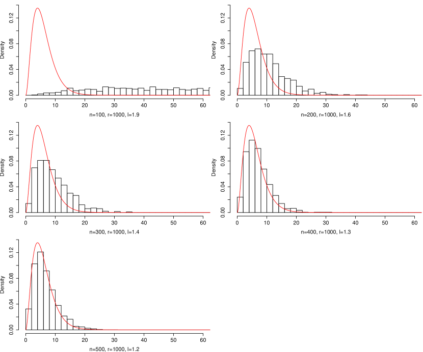
Figure 1: Histogram of Teststatistic, l=$\lambda$, the cross-validation lambda

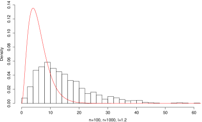
Figure 2: Histogram of Teststatistic with a tuned $\lambda_{msrL}=$l=1.2 for $n=100$

The histograms show that with increasing $n$, we get a fast convergence to the true asymptotic chi-squared distribution. It is in fact true that we could multiply the teststatistic with a constant $C_{n}\leq 1$ in order to get the histogram match the chi-squared distribution. This reflects the theory. Already with $n=400$ we get a very good approximation of the chi-quared distribution. But we see that the tuning of $\lambda_{msrL}$ is crucial for small $n$, see figure 2.

Next we try the same procedure but we are interested in what happens if we let $J$ and the active set $S_{0}$ not be the same set. Here we take $J=(1,3,4,8,10,33)$ and $\beta_{0}$ is taken from the uniform distribution on $[1,4]$ on the set $S_{0}=(2,3,5,8,11,12,14,31)$. So only the indices $J\cap S_{0}=\{3,8\}$ coincide. Figure 3 shows the results.

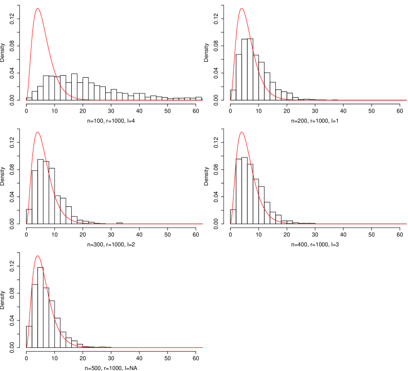
Figure 3: Histogram of Teststatistic, l=$\lambda$, the cross-validation lambda

Compared to the case where $J$ and $S_{0}$ are the same set, it seems that this setting can handle small $n$ better than in the case where all the elements of $J$ are the nonzero indices of $\beta_{0}$. So the previous case seems to be the harder case. Therefore we stick with $J=S_{0}=(1,3,4,8,10,33)$ for all the other simulations in Subsection 7.2 and 7.3.

7.2 Confidence level for an increasing $\lambda_{msrL}$

Up until now we have not looked at the behaviour for different $\lambda$. We only used the cross-validation $\lambda$. So here we look at $n=400$, $p=500$ and we take $\lambda_{msrL}=(0.01,0.11,0.21,...,2.91)$ a fixed sequence. Figure 4 shows the results.

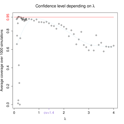
Figure 4: Average confidence level with fixed $n=400$ and $p=500$, increased $\lambda$

If we take $\lambda$ too low the behaviour breaks down. On the other hand, if $\lambda$ is too big, we will not achieve a good average confidence level. The cross-validation $\lambda$ seems to be still a bit to high. So the cross-validation $\lambda$ could be better.

7.3 Levelplot for n and p

Not let us look at an overview of alot of different settings. We will use the levelplot to present the results Here we use the cross-validation $\lambda$. We let $n$ and $p$ increase and look again at the average coverage of the confidence interval (average over the $1000$ simulations for each gridpoint). The border between high and low dimensional cases is marked by the white line in figure 5. Increasing $p$ does not worsen the procedure too much, which is very good. And, as expected, increasing the number of observations $n$ increases ”the accuracy” of the average confidence interval.

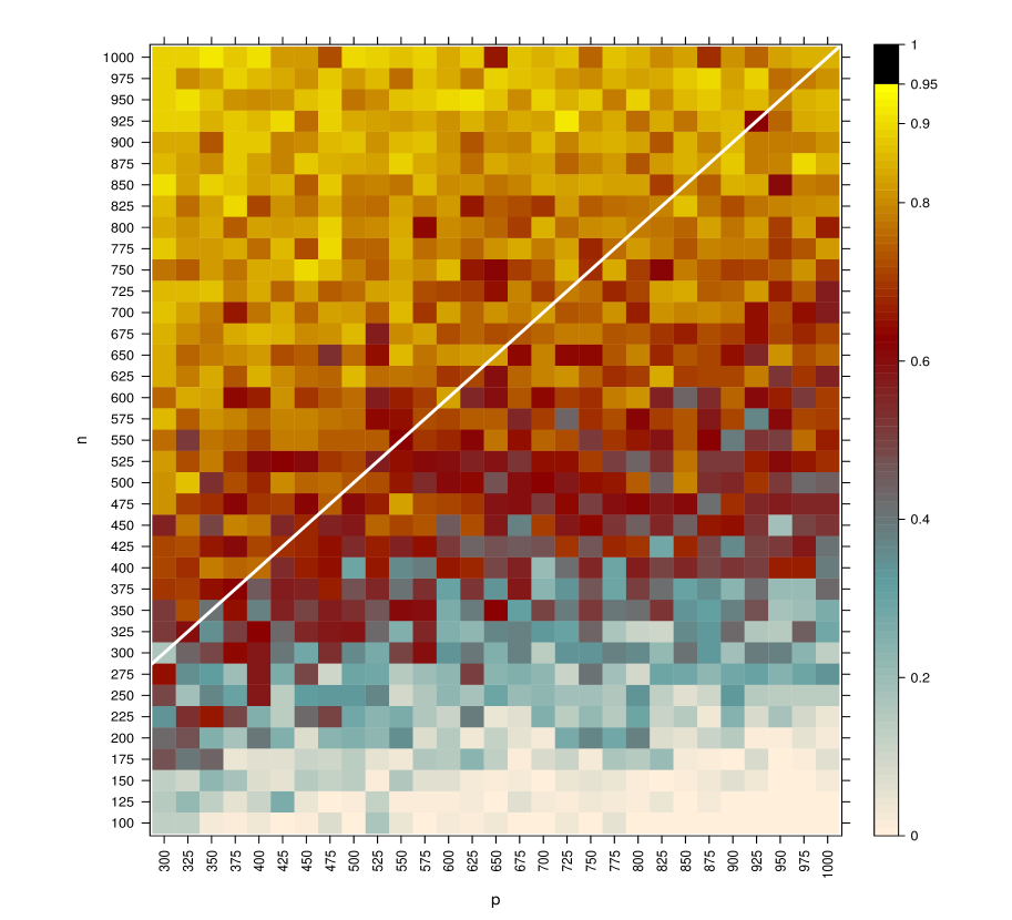
Figure 5: Levelplot of average confidence level for a grid $n,p$

8 Discussion

We have presented a method for constructing confidence sets for groups of variables which does not impose sparsity conditions on the input matrix $X$. The idea is to use a loss function based on the nuclear norm of the matrix of residuals. We called this the multivariate square-root Lasso as it is an extension of the square-root Lasso in the multivariate case.

It is easy to see that when the groups are large, one needs the $\ell_{2}$-norm of the remainder term $\|{\rm rem}\|^{2}$ in Theorem 3.1 to be of small order $\sqrt{|J|}$ in probability, using the representation $\chi^{2}_{|J|}=|J|+O_{{\rm I\hskip-1.54001ptP}}(\sqrt{J})$. This leads to the requirement that $\sqrt{n}\lambda\|\hat{\beta}_{-J}-\beta_{j}^{0}\|_{1}/\sigma_{0}=o_{{\rm I\hskip-1.54001ptP}}(1/|J|^{1/4})$, i.e., that it decreases faster for large groups. The paper Mitra and Zhang (2014) introduces a different scheme for confidence sets, where there is no dependence on group size in the remainder term after the normalization for large groups. Their idea is to use a group Lasso with a nuclear norm type of penalty on $\Gamma_{J}$ instead of the $\ell_{1}$-norm $\|\Gamma_{J}\|_{1}$ as we do in Theorem 3.1. Combining the approach of Mitra and Zhang (2014) with the result of Theorem 6.1 leads to a new remainder term which after normalization for large groups does not depend on group size and does not rely on sparsity assumptions on the design $X$.

The choice of the tuning parameter $\lambda$ for the construction used in Theorem 3.1 is as yet an open problem. When one is willing to assume certain sparsity assumptions such that a bound for $\|\hat{\beta}-\beta^{0}\|_{1}$ is available, the tuning parameter can be chosen by trading off the size of the confidence set and the bias. When the rows of $X$ are i.i.d. random variables, a choice for $\lambda$ of order $\sqrt{\log p/n}$ is theoretically justified under certain conditions. Finally, smaller $\lambda$ give more conservative confidence intervals. Thus, increasing $\lambda$ will give one a “solution path” of significant variables entering and exiting, where the number of “significant” variables increases. If one aims at finding potentially important variables, one might want to choose a cut-off level here, i.e. choose $\lambda$ in such a way that the number of “significant” variables is equal to a prescribed number. However, we have as yet no theory showing such a data-dependent choice of $\lambda$ is meaningful.

A given value for $\lambda$ may yield sets which do not have the approximate coverage. These sets can nevertheless be viewed as giving a useful importance measure for the variables, an importance measure which avoids the possible problems of other methods for accessing accuracy. For example, when applied to all variables (after grouping) the confidence sets clearly also give results for the possibly weak variables. This is in contrast to post-model selection where the variables not selected are no longer under consideration.

9 Proofs

9.1 Proof for the result for the multivariate square-root Lasso in Subsection 2.2

Proof of Lemma 1. Let us write, for each $p\times q$ matrix $B$, the residuals as $\Sigma(B):=(Y-XB)^{T}(Y-XB)/n$. Let $\Sigma_{\rm min}(B)$ be the minimizer of

$${\rm trace}(\Sigma(B)\Sigma^{-1/2})+{\rm trace}(\Sigma^{1/2})$$ (14)

over $\Sigma$. Then $\Sigma_{\rm min}(B)$ equals $\Sigma(B)$. To see this we invoke the reparametrization $\Omega:=\Sigma^{-1/2}$ so that $\Sigma^{1/2}=\Omega^{-1}$. We now minimize

$${\rm trace}(\Sigma(B)\Omega)+{\rm trace}(\Omega^{-1})$$

over $\Omega>0$. The matrix derivative with respect to $\Omega$ of ${\rm trace}(\Sigma(B)\Omega)$ is $\Sigma(B)$. The matrix derivative of ${\rm trace}(\Omega^{-1})$ with respect to $\Omega$ is equal to $-\Omega^{-2}$. Hence the minimizer $\Omega_{\rm min}(B)$ satisfies the equation

$$\Sigma(B)-\Omega_{\rm min}^{-2}(B)=0,$$

giving

$$\Omega_{\rm min}(B)=\Sigma^{-1/2}(B).$$

so that

$$\Sigma_{\rm min}(B)=\Omega_{\rm min}^{-2}(B)=\Sigma(B).$$

Inserting this solution back in (14) gives $2{\rm trace}(\Sigma^{1/2}(B))$ which is equal to $2\|Y-XB\|_{\rm nuclear}/\sqrt{n}$. This proves the first part of the lemma.

Let now for each $\Sigma>0$, $B(\Sigma)$ be the minimizer of

$${\rm trace}(\Sigma(B)\Sigma^{-1/2})+2\lambda_{0}\|B\|_{1}.$$

By sub-differential calculus we have

$$X^{T}(Y-XB)\Sigma^{-1/2}/n=\lambda_{0}Z(\Sigma)$$

where $\|Z(\Sigma)\|_{\infty}\leq 1$ and $Z_{k,j}(\Sigma))={\rm sign}(B_{k,j}(\Sigma))$ if $B_{k,j}(\Sigma)\not=0$ ($k=1,\ldots,p$, $j=1,\ldots q$). The KKT-conditions (5) follow from $\hat{B}=B(\hat{\Sigma})$. $\sqcup\mkern-12.0mu\sqcap$

9.2 Proof of the main result in Subsection 3.2

Proof of Theorem 3.1. We have

$$M(\hat{b}_{J}-\hat{\beta}_{J})=\hat{T}_{J}^{-1/2}(X_{J}-X_{-J}\hat{\Gamma}_{J})^{T}\epsilon/\sqrt{n}-\hat{T}_{J}^{-1/2}(X_{J}-X_{-J}\hat{\Gamma}_{J})^{T}X(\hat{\beta}-\beta^{0})/\sqrt{n}$$

$$=\hat{T}_{J}^{-1/2}(X_{J}-X_{-J}\hat{\Gamma}_{J})^{T}\epsilon/\sqrt{n}-\hat{T}_{J}^{-1/2}(X_{J}-X_{-J}\hat{\Gamma}_{J})^{T}X_{J}(\hat{\beta}_{J}-\beta_{J}^{0})/\sqrt{n}$$

$$-\hat{T}_{J}^{-1/2}(X_{J}-X_{-J}\hat{\Gamma}_{J})^{T}X_{-J}(\hat{\beta}_{-J}-\beta_{-J}^{0})/\sqrt{n}$$

$$=\hat{T}_{J}^{-1/2}(X_{J}-X_{-J}\hat{\Gamma}_{J})^{T}\epsilon/\sqrt{n}-M(\hat{\beta}_{J}-\beta_{J}^{0})-\sqrt{n}\lambda\hat{Z}_{J}^{T}(\hat{\beta}_{-J}-\beta_{-J}^{0})$$

where we invoked the KKT-conditions (9). We thus arrive at

$$M(\hat{b}_{J}-\beta_{J}^{0})=\hat{T}_{J}^{-1/2}(X_{J}-X_{-J}\hat{\Gamma}_{J})^{T}\epsilon/\sqrt{n}+\sigma_{0}{\rm rem},$$ (15)

where

$${\rm rem}=-\sqrt{n}\lambda\hat{Z}_{J}^{T}(\hat{\beta}_{-J}-\beta_{-J}^{0})/\sigma_{0}.$$

The co-variance matrix of the first term $\hat{T}_{J}^{-1/2}(X_{J}-X_{-J}\hat{\Gamma}_{J})^{T}\epsilon/\sqrt{n}$ in (15) is equal to

$$\sigma_{0}^{2}\hat{T}_{J}^{-1/2}(X_{J}-X_{-J}\hat{\Gamma}_{J})^{T}(X_{J}-X_{-J}\hat{\Gamma}_{J})\hat{T}_{J}^{-1/2}/n=\sigma_{0}^{2}I$$

where $I$ is the identity matrix with dimensions $|J|\times|J|$. It follows that this term is $|J|$-dimensional standard normal scaled with $\sigma_{0}$. The remainder term can be bounded using the dual norm inequality for each entry:

$$|{\rm rem}_{j}|\leq\sqrt{n}\lambda\max_{k\notin J}|(\hat{Z}_{J})_{k,j}|\|\hat{\beta}_{-J}-\beta_{-J}^{0}\|_{1}/\sigma_{0}\leq\sqrt{n}\lambda\|\hat{\beta}_{-J}-\beta_{-J}^{0}\|_{1}/\sigma_{0}$$

since by the KKT-conditions (9), we have $\|\hat{Z}_{J}\|_{\infty}\leq 1$. $\sqcup\mkern-12.0mu\sqcap$

9.3 Proofs of the theoretical result for the square-root Lasso in Section 4

Proof of Lemma 2. Without loss of generality we can assume $\sigma_{0}^{2}=1$. From Laurent and Massart (2000) we know that for all $t>0$

$${\rm I\hskip-2.20001ptP}\biggl{(}\|\epsilon\|_{n}^{2}\leq 1-2\sqrt{t/n}\biggl{)}\leq\exp[-t]$$

and

$${\rm I\hskip-2.20001ptP}\biggl{(}\|\epsilon\|_{n}^{2}\geq 1+2\sqrt{t/n}+2t/n\biggl{)}\leq\exp[-t].$$

Apply this with $t=\log(1/{\underline{\alpha}})$ and $t=\log(1/\bar{\alpha})$ respectively. Moreover $X_{j}^{T}\epsilon/n\sim{\cal N}(0,1/n)$ for all $j$. Hence for all $t>0$

$${\rm I\hskip-2.20001ptP}\biggl{(}|X_{j}^{T}\epsilon|/n\geq\sqrt{2t/n}\biggl{)}\leq 2\exp[-t],\ \forall\ j.$$

It follows that

$${\rm I\hskip-2.20001ptP}\biggl{(}\|X^{T}\epsilon\|_{\infty}/n\geq\sqrt{2(t+\log(2p))/n}\biggl{)}\leq\exp[-t].$$

$\sqcup\mkern-12.0mu\sqcap$

Proof of Lemma 3. Suppose $\hat{R}\leq R$ and $\|\epsilon\|_{n}\geq{\underline{\sigma}}$. First we note that the inequality (11) gives

$$\lambda_{0}\|\beta^{0}\|_{1}/\|\epsilon\|_{n}\leq 2\biggl{(}\sqrt{1+(\eta/2)^{2}}-1\biggr{)}.$$

For the upper bound for $\|\hat{\epsilon}\|_{n}$ we use that

$$\|\hat{\epsilon}\|_{n}+\lambda_{0}\|\hat{\beta}\|_{1}\leq\|\epsilon\|_{n}+\lambda_{0}\|\beta^{0}\|_{1}$$

by the definition of the estimator. Hence

$$\|\hat{\epsilon}\|_{n}\leq\|\epsilon\|_{n}+\lambda_{0}\|\beta^{0}\|_{1}\leq\biggl{[}1+2\biggl{(}\sqrt{1+(\eta/2)^{2}}-1\biggr{)}\biggr{]}\|\epsilon\|_{n}\leq(1+\eta)\|\epsilon\|_{n}.$$

For the lower bound for $\|\hat{\epsilon}\|_{n}$ we use the convexity of both the loss function and the penalty. Define

$$\alpha:={\eta\|\epsilon\|_{n}\over\eta\|\epsilon\|_{n}+\|X(\hat{\beta}-\beta^{0})\|_{n}}.$$

Note that $0<\alpha\leq 1$. Let $\hat{\beta}_{\alpha}$ be the convex combination $\hat{\beta}_{\alpha}:=\alpha\hat{\beta}+(1-\alpha)\beta^{0}$. Then

$$\|X(\hat{\beta}_{\alpha}-\beta^{0})\|_{n}=\alpha\|X(\hat{\beta}-\beta^{0})\|_{n}={\eta\|\epsilon\|_{n}\|X(\hat{\beta}-\beta^{0})\|_{n}\over\eta\|\epsilon\|_{n}+\|X(\hat{\beta}-\beta^{0})\|_{n}}\leq\eta\|\epsilon\|_{n}.$$

Define $\hat{\epsilon}_{\alpha}:=Y-X\hat{\beta}_{\alpha}$. Then, by convexity of $\|\cdot\|_{n}$ and $\|\cdot\|_{1}$,

$$\|\hat{\epsilon}_{\alpha}\|_{n}+\lambda_{0}\|\hat{\beta}_{\alpha}\|_{1}\leq\alpha\|\hat{\epsilon}\|_{n}+\alpha\lambda_{0}\|\hat{\beta}\|_{1}+(1-\alpha)\|\epsilon\|_{n}+(1-\alpha)\lambda_{0}\|\beta^{0}\|_{1}$$

$$\leq\|\epsilon\|_{n}+\lambda_{0}\|\beta^{0}\|_{1}$$

where in the last step we again used that $\hat{\beta}$ minimizes $\|Y-X\beta\|_{n}+\lambda_{0}\|\beta\|_{1}$. Taking squares on both sides gives

$$\|\hat{\epsilon}_{\alpha}\|_{n}^{2}+2\lambda_{0}\|\hat{\beta}_{\alpha}\|_{1}\|\hat{\epsilon}_{\alpha}\|_{n}+\lambda_{0}^{2}\|\hat{\beta}_{\alpha}\|_{1}^{2}\leq\|\epsilon\|_{n}^{2}+2\lambda_{0}\|\beta^{0}\|_{1}\|\epsilon\|_{n}+\lambda_{0}^{2}\|\beta^{0}\|_{1}^{2}.$$ (16)

But

$$\|\hat{\epsilon}_{{\alpha}}\|_{n}^{2}=\|\epsilon\|_{n}^{2}-2\epsilon^{T}X(\hat{\beta}_{\alpha}-\beta^{0})/n+\|X(\hat{\beta}_{\alpha}-\beta^{0})\|_{n}^{2}$$

$$\geq\|\epsilon\|_{n}^{2}-2R\|\hat{\beta}_{\alpha}-\beta^{0}\|_{1}\|\epsilon\|_{n}+\|X(\hat{\beta}_{\alpha}-\beta^{0})\|_{n}^{2}$$

$$\geq\|\epsilon\|_{n}^{2}-2R\|\hat{\beta}_{\alpha}\|_{1}\|\epsilon\|_{n}-2R\|\beta^{0}\|_{1}\|\epsilon\|_{n}+\|X(\hat{\beta}_{\alpha}-\beta^{0})\|_{n}^{2}.$$

Moreover, by the triangle inequality

$$\|\hat{\epsilon}_{\alpha}\|_{n}\geq\|\epsilon\|_{n}-\|X(\hat{\beta}_{\alpha}-\beta^{0})\|_{n}\geq(1-\eta)\|\epsilon\|_{n}.$$

Inserting these two inequalities into (16) gives

$$\|\epsilon\|_{n}^{2}-2R\|\hat{\beta}_{\alpha}\|_{1}\|\epsilon\|_{1}-2R\|\beta^{0}\|_{1}\|\epsilon\|_{n}+\|X(\hat{\beta}_{\alpha}-\beta^{0})\|_{n}^{2}+2\lambda_{0}(1-\eta)\|\hat{\beta}_{\alpha}\|_{1}\|\epsilon\|_{n}+\lambda_{0}^{2}\|\hat{\beta}_{\alpha}\|_{1}^{2}$$

$$\leq\|\epsilon\|_{n}^{2}+2\lambda_{0}\|\beta^{0}\|_{1}\|\epsilon\|_{n}+\lambda_{0}^{2}\|\beta^{0}\|_{1}^{2}$$

which implies by the assumption $\lambda_{0}(1-\eta)\geq R$

$$\|X(\hat{\beta}_{\alpha}-\beta^{0})\|_{n}^{2}\leq 2(\lambda_{0}+R)\|\beta^{0}\|_{1}\|\epsilon\|_{1}+\lambda_{0}^{2}\|\beta^{0}\|_{1}^{2}.$$

$$\leq 4\lambda_{0}\|\beta^{0}\|_{1}\|\epsilon\|_{1}+\lambda_{0}^{2}\|\beta^{0}\|_{1}^{2}$$

where in the last inequality we used $R\leq(1-\eta)\lambda_{0}\leq\lambda_{0}$. But continuing we see that we can write the last expression as

$$4\lambda_{0}\|\beta^{0}\|_{1}\|\epsilon\|_{1}+\lambda_{0}^{2}\|\beta^{0}\|_{1}^{2}=\biggl{(}(\lambda_{0}\|\beta_{0}\|_{1}/\|\epsilon_{n}\|_{n}+2)^{2}-4\biggr{)}\|\epsilon\|_{n}^{2}.$$

Again invoke the $\ell_{1}$-sparsity condition

$$\lambda_{0}\|\beta^{0}\|_{1}/\|\epsilon\|_{n}\leq 2\biggl{(}\sqrt{1+(\eta/2)^{2}}-1\biggr{)}$$

to get

$$\biggl{(}(\lambda_{0}\|\beta_{0}\|_{1}/\|\epsilon_{n}\|_{n}+2)^{2}-4\biggr{)}\|\epsilon\|_{n}^{2}\leq{\eta^{2}\over 4}\|\epsilon\|_{n}^{2}.$$

We thus established that

$$\|X(\hat{\beta}_{\alpha}-\beta^{0})\|_{n}\leq{\eta\|\epsilon\|_{n}\over 2}.$$

Rewrite this to

$${\eta\|\epsilon\|_{n}\|X(\hat{\beta}-\beta^{0})\|_{n}\over\eta\|\epsilon\|_{n}+\|X(\hat{\beta}-\beta^{0})\|_{n}}\leq{\eta\|\epsilon\|_{n}\over 2},$$

and rewrite this in turn to

$$\eta\|\epsilon\|_{n}\|X(\hat{\beta}-\beta^{0})\|_{n}\leq{\eta^{2}\|\epsilon\|_{n}^{2}\over 2}+{\eta\|\epsilon\|_{n}\|X(\hat{\beta}-\beta^{0})\|_{n}\over 2}$$

or

$$\|X(\hat{\beta}-\beta^{0})\|_{n}\leq\eta\|\epsilon\|_{n}.$$

But then, by repeating the argument, also

$$\|\hat{\epsilon}\|_{n}\geq\|\epsilon\|_{n}-\|X(\hat{\beta}-\beta^{0})\|_{n}\geq(1-\eta)\|\epsilon\|_{n}.$$

$\sqcup\mkern-12.0mu\sqcap$

Proof of Theorem 4.1. Throughout the proof we suppose $\hat{R}\leq R$ and $\|\epsilon\|_{n}\geq{\underline{\sigma}}$. Define the Gram matrix $\hat{\Sigma}:=X^{T}X/n$. Let $\beta\in\mathbb{R}^{p}$ and $S:=S_{\beta}=\{j:\ \beta_{j}\not=0\}$. If

$$(\hat{\beta}-\beta)^{T}\hat{\Sigma}(\hat{\beta}-\beta^{0})\leq-\delta\underline{\lambda}\|\hat{\beta}-\beta\|_{1}\|\epsilon\|_{n}$$

we find

$$2\delta\underline{\lambda}\|\hat{\beta}-\beta\|_{1}\|\epsilon\|_{n}+\|X(\hat{\beta}-\beta^{0})\|_{n}^{2}$$

$$=2\delta\underline{\lambda}\|\hat{\beta}-\beta\|_{1}\|\epsilon\|_{n}+\|X(\beta-\beta^{0})\|_{n}^{2}-\|X(\beta-\hat{\beta})\|_{n}^{2}+2(\hat{\beta}-\beta)^{T}\hat{\Sigma}(\hat{\beta}-\beta^{0})$$

$$\leq\|X(\beta-\beta^{0})\|_{n}^{2}.$$

So then we are done.

Suppose now that

$$(\hat{\beta}-\beta)^{T}\hat{\Sigma}(\hat{\beta}-\beta^{0})\geq-\delta\underline{\lambda}\|\hat{\beta}-\beta\|_{1}\|\epsilon\|_{n}.$$

By the KKT-conditions (3)

$$(\hat{\beta}-\beta)^{T}\hat{\Sigma}(\hat{\beta}-\beta^{0})+\lambda_{0}\|\hat{\beta}\|_{1}\|\hat{\epsilon}\|_{n}\leq\epsilon^{T}X(\hat{\beta}-\beta)/n+\lambda_{0}\|\beta\|_{1}\|\hat{\epsilon}\|_{n}.$$

By the dual norm inequality and since $\hat{R}\leq R$

$$|\epsilon^{T}X(\hat{\beta}-\beta)|/n\leq R\|\hat{\beta}-\beta\|_{1}\|\epsilon\|_{n}.$$

Thus

$$(\hat{\beta}-\beta)^{T}\hat{\Sigma}(\hat{\beta}-\beta^{0})+\lambda_{0}\|\hat{\beta}\|_{1}\|\hat{\epsilon}\|_{n}\leq R\|\hat{\beta}-\beta\|_{1}\|\epsilon\|_{n}+\lambda_{0}\|\beta\|_{1}\|\hat{\epsilon}\|_{n}.$$

This implies by the triangle inequality

$$(\hat{\beta}-\beta)^{T}\hat{\Sigma}(\hat{\beta}-\beta^{0})+(\lambda_{0}\|\hat{\epsilon}\|_{n}-R\|\epsilon\|_{n})\|\hat{\beta}_{-S}\|_{1}\leq(\lambda_{0}\|\hat{\epsilon}\|_{n}+R\|\epsilon\|_{n})\|\hat{\beta}_{S}-\beta\|_{1}.$$

We invoke the result of Lemma 3 which says that that $(1-\eta)\|\epsilon\|_{n}\leq\|\hat{\epsilon}\|_{n}\leq(1+\eta)\|\epsilon\|_{n}$. This gives

$$(\hat{\beta}-\beta)^{T}\hat{\Sigma}(\hat{\beta}-\beta^{0})+\underline{\lambda}\|\hat{\beta}_{-S}\|_{1}\|\epsilon\|_{n}\leq(\lambda_{0}(1+\eta)+R)\|\hat{\beta}_{S}-\beta\|_{1}\|\epsilon\|_{n}.$$ (17)

Since $(\hat{\beta}-\beta)^{T}\hat{\Sigma}(\hat{\beta}-\beta^{0})\geq-\delta\underline{\lambda}\|\epsilon\|_{n}\|\hat{\beta}-\beta\|_{1}$ this gives

$$(1-\delta)\underline{\lambda}\|\hat{\beta}_{-S}\|_{1}\|\epsilon\|_{n}\leq(\lambda_{0}(1+\eta)+R+\delta\underline{\lambda})\|\hat{\beta}_{S}-\beta\|_{1}\|\epsilon\|_{n}=\bar{\lambda}\|\hat{\beta}_{S}-\beta\|_{1}\|\epsilon\|_{n}.$$

or

$$\|\hat{\beta}_{-S}\|_{1}\leq L\|\hat{\beta}_{S}-\beta\|_{1}.$$

But then

$$\|\hat{\beta}_{S}-\beta\|_{1}\leq\sqrt{|S|}\|X(\hat{\beta}-\beta)\|_{n}/\hat{\phi}(L,S).$$ (18)

Continue with inequality (17) and apply the inequality $ab\leq(a^{2}+b^{2})/2$ which holds for all real valued $a$ and $b$:

$$(\hat{\beta}-\beta)\hat{\Sigma}(\hat{\beta}-\beta^{0})+\underline{\lambda}\|\hat{\beta}_{-S}\|_{1}\|\epsilon\|_{n}+\delta\underline{\lambda}\|\hat{\beta}_{S}-\beta\|_{1}\|\epsilon\|_{n}$$

$$\leq\bar{\lambda}\|\epsilon\|_{n}\sqrt{|S|}\|X(\hat{\beta}-\beta)\|_{n}/\hat{\phi}(L,S)$$

$$\leq{1\over 2}{\bar{\lambda}}^{2}{|S|\|\epsilon\|_{n}^{2}\over\hat{\phi}^{2}(L,S)}+{1\over 2}\|X(\hat{\beta}-\beta)\|_{n}^{2}.$$

Since

$$2(\hat{\beta}-\beta)^{T}\hat{\Sigma}(\hat{\beta}-\beta^{0})=\|X(\hat{\beta}-\beta^{0})\|_{n}^{2}-\|X(\beta-\beta^{0})\|_{n}^{2}+\|X(\hat{\beta}-\beta)\|_{n}^{2},$$

we obtain

$$\|X(\hat{\beta}-\beta^{0})\|_{n}^{2}+2\underline{\lambda}\|\hat{\beta}_{-S}\|_{1}\|\epsilon\|_{n}+2\delta\underline{\lambda}\|\hat{\beta}_{S}-\beta\|_{1}\|\epsilon\|_{n}$$

$$\leq\|X(\beta-\beta^{0})\|_{n}^{2}+{\bar{\lambda}}^{2}|S|\|\epsilon\|_{n}^{2}/\hat{\phi}^{2}(L,S).$$

$\sqcup\mkern-12.0mu\sqcap$

9.4 Proofs of the illustration assuming (weak) sparsity in Section 5

Proof of Lemma 4. Define $\lambda_{*}:={\bar{\lambda}}\|\epsilon\|_{n}/\hat{\Lambda}_{\rm max}(S_{0})$ and for $j=1,\ldots,p$,

$$\beta_{j}^{*}=\beta_{j}^{0}{\rm l}\{|\beta_{j}^{0}|>\lambda_{*}\}.$$

Then

$$\|X(\beta^{*}-\beta^{0})\|_{n}^{2}\leq\hat{\Lambda}_{\rm max}^{2}(S_{0})\|\beta^{*}-\beta^{0}\|_{2}^{2}\leq\hat{\Lambda}_{\rm max}^{2}(S_{0})\lambda_{*}^{2-r}\rho_{r}^{r}$$

$$=\bar{\lambda}^{2-r}\hat{\Lambda}_{\rm max}^{r}(S_{0})\rho_{r}^{r}\|\epsilon\|_{n}^{2-r}\leq\bar{\lambda}^{2-r}\hat{\Lambda}_{\rm max}^{r}(S_{0})\rho_{r}^{r}\|\epsilon\|_{n}^{2-r}/\hat{\phi}^{2}(L,S_{*})$$

where in the last inequality we used $\hat{\phi}(L,S_{*})\leq 1$. Moreover, noting that $S_{\beta^{*}}=\hat{S}_{*}=\{j:\ |\beta_{j}^{0}|>\lambda^{*}\}$ we get

$$|S_{\beta^{*}}|\leq\lambda_{*}^{-r}\rho_{r}^{r}=\bar{\lambda}^{-r}\|\epsilon\|_{n}^{-r}\hat{\Lambda}_{\rm max}^{r}(S_{0}).$$

Thus

$$\bar{\lambda}^{2}|S_{\beta^{*}}|\|\epsilon\|_{n}^{2}/\hat{\phi}^{2}(L,S_{\beta^{*}})\leq\bar{\lambda}^{2-r}\hat{\Lambda}_{\rm max}^{r}(S_{0})\rho_{r}^{r}\|\epsilon\|_{n}^{2-r}/\hat{\phi}^{2}(L,\hat{S}_{*}).$$

Moreover

$$\|\beta^{*}-\beta_{0}\|_{1}\leq\lambda_{*}^{1-r}\rho_{r}^{r}={\bar{\lambda}}^{1-r}\|\epsilon\|_{n}^{1-r}\hat{\Lambda}_{\rm max}^{r}(S_{0})/\hat{\phi}^{2}(L,\hat{S}_{*}),$$

since $\hat{\phi}^{2}(L,\hat{S}_{*})/\hat{\Lambda}_{\rm max}(S_{0})\leq 1$. $\sqcup\mkern-12.0mu\sqcap$

Proof of Lemma 5. The $\ell_{1}$-sparsity condition (11) holds with $\eta\leq 1/3$. Theorem 4.1 with $\lambda_{0}(1-\eta)=2R$ gives ${\underline{\lambda}}=\lambda_{0}(1-\eta)-R=R$ and $3R\leq\bar{\lambda}=\lambda_{0}(1+\eta)+R+\delta{\underline{\lambda}}\leq(5+\delta)R$. We take $\delta=1/7$. Then $L=\bar{\lambda}/((1-\delta){\underline{\lambda}})\leq(5+\delta)/(1-\delta)=6$. Set $\hat{S}_{*}:=\{j:\ |\beta_{j}^{0}|>\bar{\lambda}\|\epsilon\|_{n}/\hat{\Lambda}_{\rm max}(S_{0})\}$. On the set where $\|\epsilon\|_{n}\geq{\underline{\sigma}}$ we have $\hat{S}_{*}\subset S_{*}$ since $\bar{\lambda}\geq 3R$. We also have $\bar{\lambda}/(\delta{\underline{\lambda}})\leq 6^{2}$. Hence, using the arguments of Lemma 4 and the result of Theorem 4.1, we get on the set $\hat{R}\leq R$ and $\|\epsilon\|_{n}\geq{\underline{\sigma}}$,

$${\|\hat{\beta}-\beta^{0}\|_{1}\over\|\epsilon\|_{n}}\leq{\bar{\lambda}}^{1-r}\biggl{(}1+{6^{2}\hat{\Lambda}_{\rm max}^{r}(S_{0})\over\hat{\phi}^{2}(6,S_{*})}\biggr{)}\biggr{(}{\rho_{r}\over\|\epsilon\|_{n}}\biggr{)}^{r}.$$

Again, we can bound here $1/\|\epsilon\|_{n}$ by $1/{\underline{\sigma}}$. We can moreover bound $\bar{\lambda}$ by $6R$. Next we see that on the set where $\hat{R}\leq R$ and $\|\epsilon\|_{n}\geq{\underline{\sigma}}$, by Lemma 3,

$$\hat{\sigma}\geq(1-\eta)\|\epsilon\|_{n}\geq(1-\eta){\underline{\sigma}}.$$

The $\ell_{0}$-bound follows in the same way, inserting $\beta=\beta^{0}$ in Theorem 3.1. Invoke Lemma 2 to show that the set $\{\hat{R}\leq R\cap\|\epsilon\|_{n}\geq\underline{\sigma}\}$ has probability at least $1-\alpha_{0}-{\underline{\alpha}}$. $\sqcup\mkern-12.0mu\sqcap$

9.5 Proof of the extension to structured sparsity in Section 6

Proof of Theorem 6.1. This follows from exactly the same arguments as used in the proof of Theorem 3.1 as the KKT-conditions (9) with general norm $\Omega$ imply that

$$\|X_{-J}^{T}(X_{J}-X_{-J}\hat{\Gamma}_{J})\hat{T}_{J}^{-1/2}/n\|_{\infty,\Omega_{*}}\leq\lambda.$$

$\sqcup\mkern-12.0mu\sqcap$

References

- Bach [2010] F. Bach. Structured sparsity-inducing norms through submodular functions. In Advances in Neural Information Processing Systems (NIPS), volume 23, pages 118–126, 2010.
- Belloni et al. [2011] A. Belloni, V. Chernozhukov, and L. Wang. Square-root Lasso: pivotal recovery of sparse signals via conic programming. Biometrika, 98(4):791–806, 2011.
- Belloni et al. [2013a] A. Belloni, V. Chernozhukov, and K. Kato. Uniform postselection inference for LAD regression models, 2013a. arXiv:1306.0282.
- Belloni et al. [2013b] A. Belloni, V. Chernozhukov, and Y. Wei. Honest confidence regions for logistic regression with a large number of controls, 2013b. arXiv:1306.3969.
- Belloni et al. [2014] A. Belloni, V. Chernozhukov, and C. Hansen. Inference on treatment effects after selection among high-dimensional controls. Review of Economic Studies, 81(2):608–650, 2014.
- Bickel et al. [2009] P. Bickel, Y. Ritov, and A. Tsybakov. Simultaneous analysis of Lasso and Dantzig selector. Annals of Statistics, 37:1705–1732, 2009.
- Bunea et al. [2013] F. Bunea, J. Lederer, and Y. She. The group square-root Lasso: theoretical properties and fast algorithms, 2013. arXiv:1302.0261.
- Javanmard and Montanari [2013] A. Javanmard and A. Montanari. Hypothesis testing in high-dimensional regression under the Gaussian random design model: asymptotic theory, 2013. arXiv:1301.4240v1.
- Koltchinskii et al. [2011] V. Koltchinskii, K. Lounici, and A.B. Tsybakov. Nuclear-norm penalization and optimal rates for noisy low-rank matrix completion. Annals of Statistics, 39(5):2302–2329, 2011.
- Laurent and Massart [2000] B. Laurent and P. Massart. Adaptive estimation of a quadratic functional by model selection. Annals of Statistics, pages 1302–1338, 2000.
- Lounici et al. [2011] K. Lounici, M. Pontil, S. van de Geer, and A.B. Tsybakov. Oracle inequalities and optimal inference under group sparsity. Annals of Statistics, 39:2164–2204, 2011.
- Mitra and Zhang [2014] R. Mitra and C.-H. Zhang. The benefit of group sparsity in group inference with de-biased scaled group Lasso, 2014. arXiv:1412.4170.
- Obozinski and Bach [2012] G. Obozinski and F. Bach. Convex relaxation for combinatorial penalties, 2012. arXiv:1205.1240.
- Sun and Zhang [2012] T. Sun and C.-H. Zhang. Scaled sparse linear regression. Biometrika, 99:879–898, 2012.
- Sun and Zhang [2013] T. Sun and C.-H. Zhang. Sparse matrix inversion with scaled lasso. The Journal of Machine Learning Research, 14(1):3385–3418, 2013.
- van de Geer [2014] S. van de Geer. Weakly decomposable regularization penalties and structured sparsity. Scandinavian Journal of Statistics, 41(1):72–86, 2014.
- van de Geer et al. [2014] S. van de Geer, P. Bühlmann, Y. Ritov, and R. Dezeure. On asymptotically optimal confidence regions and tests for high-dimensional models. Annals of Statistics, 42:1166–1202, 2014.
- van de Geer [2007] S.A. van de Geer. The deterministic Lasso. In JSM proceedings, 2007, 140. American Statistical Association, 2007.
- Yuan and Lin [2006] M. Yuan and Y. Lin. Model selection and estimation in regression with grouped variables. Journal of the Royal Statistical Society Series B, 68:49, 2006.
- Zhang and Zhang [2014] C.-H. Zhang and S. S. Zhang. Confidence intervals for low dimensional parameters in high dimensional linear models. Journal of the Royal Statistical Society: Series B (Statistical Methodology), 76(1):217–242, 2014.