Critical-like Features of Stress Response in Frictional Packings

Abstract

The mechanical response of static, unconfined, overcompressed face centred cubic, granular arrays is studied using large-scale, discrete element method simulations. Specifically, the stress response due to the application of a localised force perturbation - the Green function technique - is obtained in granular packings generated over several orders of magnitude in both the particle friction coefficient and the applied forcing. We observe crossover behaviour in the mechanical state of the system characterised by the changing nature of the resulting stress response. The transition between anisotropic and isotropic stress response exhibits critical-like features through the identification of a diverging length scale that distinguishes the spatial extent of anisotropic regions from those that display isotropic behaviour. A multidimensional phase diagram is constructed that parameterises the response of the system due to changing friction and force perturbations.

I Introduction

Granular materials are ubiquitous throughout industry and nature and constitute myriad materials ranging from snowpacks, planetary regoliths, silos filled with grain, through to pharmaceutical pills and ceramic components. Yet predicting the mechanical properties of a given granular material, such as a packing of frictional grains, is difficult due to the many factors that influence the stability of the packing. These can include microscopic features such as particle roughness, shape, and softness, to more macroscopic issues like the overall structural arrangement of the grains, density or packing fraction of the granular medium, and the properties of the container holding the material. Indeed, through a number of experimental Silva and Rajchenbach (2000); Geng et al. (2003); Serero et al. (2001); Mueggenburg et al. (2002); Spannuth et al. (2004); Reydellet and Clément (2001); Amar et al. (2011) and theoretical and computer simulation studies Otto et al. (2003); Goldenberg and Goldhirsch (2005); Gland et al. (2006); Tighe and Socolar (2008), it has emerged that a granular medium can appear to behave not only as a mechanically stable continuous elastic solid but can also exhibit strongly non-linear features characterised by highly heterogeneous stress properties. Though more recently, simulations that take into account the full preparation history of pouring a granular piling under gravity find that traditional elastoplastic continuum models are able to reproduce the stress-dip phenomena Zheng and Yu (2014). However, in the absence of such knowledge it is unclear how best to categorise any given granular packing. Yet, despite these complications, there are several methods that can be used to probe the mechanical robustness of the material.

One protocol readily implemented that provides just such information on the nature of the stress state of a granular medium is the Green function technique: apply a localised, point force to the packing and observe the resulting stress profile in response to the perturbation Timoshenko and Goodier (1970). A schematic of the procedure is shown in Figure 1. This technique has been implemented in experiments Geng et al. (2003) and computer simulations Atman et al. (2005); Goldenberg and Goldhirsch (2005, 2008) to show that two dimensional (2d) disc packings tend to agree with traditional, isotropic, elasticity theory Johnson (1987); Timoshenko and Goodier (1970); Landau and Lifshitz (1986) when particle friction is large. That is to say, the maximum in the measured stress profile remains directly ‘below’ the location of the perturbing force and is often termed “one-peak” response in reference to two dimensional studies. This becomes a single lobe in three dimensions (3d). However, for smoother particles, the stress response becomes highly anisotropic, exhibiting a “twin-peak” (ring profile in three dimensional packings) of maximum stress that is not directly in line with the applied force. Nevertheless, despite these differences, either type of response is generally regarded to belong to solutions of the elastic-elliptic class Otto et al. (2003); Goldenberg and Goldhirsch (2008); Jiang and Liu (2007). Furthermore, some studies Geng et al. (2003); Goldenberg and Goldhirsch (2005) have also hinted at the possibility that the response within a grain pile may change character as one looks further from the location of the perturbing source. In another study Ostojic and Panja (2006), a transition in the stress response within granular arrays is associated with a length scale though there has not been an explicit identification of the length scale nor the dependence on friction coefficient. This has important consequences as to whether a given material will indeed conform to a more isotropic or anisotropic picture, and raises the possibility that the stress state of a particulate medium may be tailored to respond differently on varying length scales. As yet there remains no method to predict a priori what the expected stress response of a three dimensional granular packing is and how the stress state of the system varies within the packing itself.

Figure 1: Implementing the force perturbation protocol referred to as the Green function technique. In this illustration, the arrow represents a downward, vertical point force applied at the middle on the top of a slab of material under interrogation. Possible stress response profiles are represented by the arcs and directed lines. The mechanical state of the systems is then inferred through monitoring the resulting stress profile along the $x$-direction at different slices in $z$. Note, this is merely a 2d visualisation of the 3d problem we discuss here.

It is precisely this issue that we address here. In an effort to reduce the large parameter space of all possible influences, we focus on what we reason are the two most dominant effects: particle friction and magnitude of the perturbing force. (The role of structural disorder was addressed previously Silbert (2010a).) This study is needed to provide a guide in the design of granular solids where they can behave as a stable solid or exhibit strongly non-linear features with tailored mechanical properties. From this study, length scales distinguishing between anisotropic from isotropic behaviours can be estimated. The organisation of this paper is as follows. The Boussinesq equations are briefly discussed in section II. The manner in which we implement the packing preparation method and the Green function technique are described in section III and summarised in Ref. Cakir and Silbert (2011). The results of this paper are presented in section IV followed by closing discussions and conclusions, section V.

II Boussinesq Equations

Isotropic linear elastic theory is based on the solutions of the elliptic differential equations of mechanical equilibrium Landau and Lifshitz (1986). For a point force ($F_{\rm app}$) applied in downward z direction to an elastic half space - the Green function technique (see Figure 1) - the solutions of the elliptic mechanical equilibrium differential equations provide the displacement field

$$u_{x}$$ ,

,

,

(1)

where, $u_{x,y,z}$ are the $x$, $y$, and $z$ displacement field components and $r=\sqrt{x^{2}+y^{2}+z^{2}}$. $\nu$ and $G$ are bulk material parameters, the Poisson ratio and modulus of rigidity, respectively. $\nu$ is restricted to the values between $-1$ and $0.5$ Landau and Lifshitz (1986). The above equations, Eqs. 1, express a displacement vector at an arbitrarily chosen point inside a solid in response to the localised force perturbation $F_{app}$.

By implementing the displacement field components into the definitions of strain and applying Hooke’s law between stress and strain, we arrive at the stress response components known as Boussinesq equations (in three dimensions) Landau and Lifshitz (1986); Johnson (1987). The origin of the coordinate system is at the application point of the applied forcing. Since the force is in the z direction the stress component characterising the response of a system is $\sigma_{zz}$, which we refer to as $\sigma$,

$$\sigma=\frac{3F_{\rm app}}{2\pi}\frac{z^{3}}{r^{5}}$$ (2)

The crucial feature of the Green function approach is in reducing the problem to a material parameter free equation, Eq. 2. The procedure we follow is through direct comparison of our simulation data with those of the Boussinesq result, Eq. 2. When we have “single-peak” behaviour (in three dimensions, a lobed profile) we attempt to fit our results. We repeat this process over our range of parameters in friction coefficients and force perturbations.

III Simulation Procedure

III.1 Packing Generation Protocol

We employ simulation domains with periodic boundary conditions to reduce the effects of confining walls which can strongly influence the nature of the stress response in small systems Cakir and Silbert (2011). From our previous studies on confined systems, we found that for a granular packing that exhibits an isotropic, elastic-like response, the response behaviour converged to the theoretical predictions for systems of linear dimension, $L>20d$, for particle diameter $d$. Therefore, for this study we generated particle configurations of size $L\approx 60d$, as a system that is suitable to mimic the response within a semi-infinite medium. We placed $N=256000$, monodisperse, inelastic spheres at the lattice points of a face centred cubic (FCC) array in the absence of gravity. The packing was then isotropically compressed under uniform pressure until the system reached a packing fraction, $\phi=0.742$, which is slightly above the hard-sphere FCC value, $\phi_{FCC}=\pi/\sqrt{18}$. Particles interact only on contact through a linear force law characterised by stiffness parameters, $k_{n}$ and $k_{t}$, for interactions normal and tangential to the contact plane where the maximum friction force is determined by the particle friction coefficient $\mu$. For this study, the particle Poisson ratio was set to, $k_{t}/k_{n}=1$. Friction is included using a standard granular dynamics routine Silbert (2010b). The normal and tangential contact forces between particles ($F_{n,t}$) are given by,

$$F_{n}$$ =

= .

(3)

where $\Delta_{ij}\equiv(r_{ij}-d)$ is the surface compression of two contacting particles and $v_{{n,t}_{ij}}$ are the relative normal and tangential velocities of two particles. $r_{ij}$ is the relative distance between particles $i$ at position $r_{i}$ and $j$ at position $r_{j}$. The effective mass, $m_{\rm eff}$ is equal to $m/2$, for particle mass $m$. $\gamma^{n,t}$ are the normal and tangential damping factors, which together with the $k_{n,t}$ and $m$ set the coefficient of restitution of the particles, which here is fixed to $\approx 0$ . $S_{ij}$ represents the integrated displacement of the contact point of the particles $i$ and $j$ while the two particles remain in contact. The Coulomb condition is written as $F_{t}\leq\mu F_{n}$. We generated static packings for different friction, ranging over several orders of magnitude, $\mu=0,0.001,0.002,0.005,0.01,0.02,0.05,0.1,0.2,0.5,1,10$. Below, we present our results in simulation units where mass, length, and force values are appropriately scaled by the particle properties: mass $m=1$, diameter $d=1$, and stiffness $k=k_{n}=k_{t}=1$.

III.2 Force Perturbation Protocol

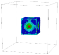
(a) (b)

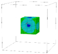
Figure 2: Simulation snapshots of the force perturbation in systems that exhibit, (a) an anisotropic, ring-like (twin-peak) response $\mu=0$ and (b) an isotropic, single lobe (single-peak) response, $\mu=1$. Each panel focuses on the central region of the packings with particles shaded by their displacement relative to the unperturbed initial state. A force perturbation was applied at the centre of the box as described in the text. Shading represents magnitude of the displacement (relative to the average for that system): blue end of spectrum corresponds to larger displacements. For the FCC particle arrangement at an overcompressed packing fraction $\phi=0.742$ used in this study.

The localised force perturbations were implemented in the following manner. We first located an approximately spherical cluster of particles within the central region of the packing that typically consisted of $<0.3\%$ of the total number of particles in the system. We then increased their diameters by a specified amount and allowed the packing to relax back into a mechanically stable state keeping the same periodic boundary conditions. The effect of this local swelling of particles is equivalent to applying a localised and isotropic perturbing force, $F_{\rm app}$, at the centre of the packing, that we varied over several orders in magnitude: $F_{\rm app}=0.0005,0.001,0.0025,0.005,0.01,0.025,0.05,0.1,0.25~{}kd$. This procedure, initially implemented in Ref. Silbert, 2010a, was motivated by several considerations. Firstly, given that we exclude gravity in this work, we preferred to avoid imposing a uni-directional force that would break the symmetry of our set up. We also reasoned that this protocol offers a practical means to implement force perturbations in real systems. As a case in point, during the course of this work, a recent experimental work has implemented a similar procedure in studies of the mechanical properties of two-dimensional granular packings Coulais et al. (2014). We have verified that the method of increasing the size of particles, located within a small region centred at origin, does indeed result in a corresponding force magnitude equal to $F_{\rm app}$, by measuring the average force over a spherical shell in the vicinity of the inflated region. Representative snapshots of how the force perturbation influences the packing are shown in Figure 2. These images display the particles occupying a sample, cubic central portion of the packing (out to 10d) for $\mu=0$ and $F_{\rm app}=0.25$ (Figure 2(a)) and $\mu=1$ and $F_{\rm app}=0.02$ (Figure 2(b)). These examples were chosen to clearly illustrate the change in response. The magnitude of particle displacements relative to their initial, unperturbed positions are indicated by a shading scale, with the blue end of the spectrum indicating larger displacements. These microdisplacements of the particles in response to the applied force indicate the reasons behind the differences between the anisotropic and isotropic response functions. In the anisotropic case, maximal particle displacements are directed along an open cone, whereas in the isotropic case the displacements ultimately form a closed ‘ball’ emanating away from the region of the perturbing source. We have verified that for the system size studied here, our results match exactly the predictions of Eq. 2 when we observe an isotropic response (which occurs for large friction and small applied force - see Figure 8).

We define the stress response as the difference between the final and initial stress states. We computed the stress in the packing before, $\sigma_{\rm i}$, and after, $\sigma_{\rm f}$, the imposition of the perturbation, so that the resulting stress response is,

$$\sigma=\sigma_{\rm f}-\sigma_{\rm i}.$$ (4)

III.3 Coarse Graining Procedure

To be able to accurately compare our simulation stress response with elasticity theories, we implement a stress computation method that connects our microscopic, discretized calculations with macroscopic, continuum length scales. A stress expression with a coarse-graining procedure developed by Goldhirsch and colleagues Goldhirsch (2010); Goldenberg and Goldhirsch (2008) gives continuum stress components. We chose a Gaussian coarse-graining function, so that the components $\alpha,\beta$ (=$x,y,z$), of the stress tensor $\sigma({\bf r})$, are obtained from,

$$\sigma_{\alpha\beta}({\bf{r}})=\frac{1}{2}\sum\limits_{i}\sum\limits_{j\neq i}F_{ij\alpha}r_{ij\beta}\int\limits_{0}^{1}\frac{ds}{(\pi^{1/2}\omega)^{3}}e^{-(\mid{\bf r}-{{\bf r}_{i}}+s{{\bf r}_{ij}}\mid/\omega)^{2}}$$ (5)

where $\omega$ is the coarse-graining length scale and ${\bf F}_{ij}$ are the contact forces between particles $i$ and $j$. This expression is normalised. The value of the coarse-graining length scale, $\omega$, is important in terms of obtaining a fine resolution and yet continuum description of stress components. Here, the particle diameter, $d$, is a suitable choice. The coarse grained stress expression, Eq. 5, is calculated on a spatial grid discretized by grid size of $0.2d$.

IV Results

IV.1 Stress Maps

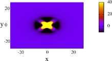
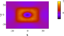
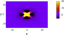
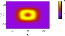
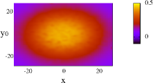
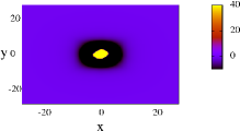
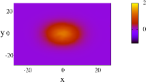
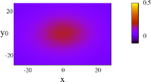
Figure 3: The stress response viewed in planes normal to the direction of the perturbing force. The origin of the coordinate system is defined as the location of the perturbing force. Here, the horizontal slices are denoted $xy$-planes and the different columns correspond to different slices in the $z$ direction. The three rows correspond to different particle friction: $\mu=0$ (top), $\mu=0.05$ (middle), and $\mu=10$ (bottom). Within each row, columns show the stress at different distances from the location of the perturbing force: left column is closest to the force. The shading scale is the same for each row but different among the columns to better reveal the stress profiles. In all cases, the applied force magnitude, $F_{app}=0.25kd$.

To make our results connect visually with existing experiments, we present our results as stress maps in different planes with respect to the perturbation source. We also plot the circularly-averaged stress as two dimensional profiles across the central section from planes that are perpendicular to the direction of the force perturbation. In Figure 3 we show stress profiles for packings with different friction subject to an applied force perturbation of a relatively large, fixed magnitude $F_{\rm app}=0.25~{}kd$. The panels of Figure 3 are arranged as follows: each row corresponds to a single friction coefficient while each column shows data at different distances from the perturbing source. We refer to these planes as ‘top’, ‘middle’, and ‘bottom’ referring to how far from the perturbation source we view the stress, with the top layer closest to the source and bottom furthest away. The left column is stress profile closest to the source (‘top’) and the right column furthest away (‘bottom’). Immediately we see how friction plays a major role in determining the response of the system. Consistent with previous studies Goldenberg and Goldhirsch (2005) we find that friction enhances the elastic nature of the response whereby the response profile remains “single peaked” at all distances from the source, with linear, isotropic elastic broadening of the profile. At zero friction, the profile is strongly anisotropic away from the source with a ring-like or “twin-peak” response, reflecting the lattice structure of the underlying packing, that persists at the largest distances. However, for intermediate friction values, the response initially resembles the zero-friction state out to a finite distance from the source then transitions to a more isotropic, single-peak response at larger distances.

IV.2 Stress Profiles

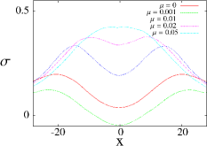
Figure 4: Circularly averaged stress profiles $\sigma$, at the ‘bottom’ layer due to applied force $F_{\rm app}=0.25kd$, for different friction coefficient $\mu$, as indicated in key.

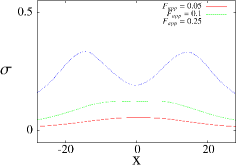
Figure 5: Circularly averaged stress profiles $\sigma$, at the bottom layer due to forces, at $\mu=0.01$, for different applied force $F_{app}$.

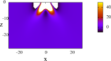
a b c

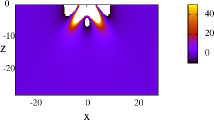
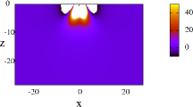
d e f

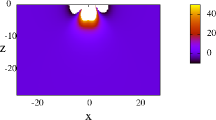
Figure 6: The influence of friction on the stress response. Profiles are viewed in planes parallel to the direction of the applied force perturbation, for a force magnitude $F_{app}=0.25kd$. Panels are particle friction values: (top left) $\mu=0$, (top middle) $\mu=0.01$, (top right) $\mu=0.05$, (bottom left) $\mu=0.5$, (bottom middle) $\mu=1$, and (bottom right) $\mu=10$.

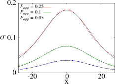
Figure 7: Circularly averaged stress profiles $\sigma$, at the bottom layer due to forces, with $\mu=10$, for different applied force $F_{app}$ (color dashed lines) and the fittings to the Boussinesq equation (solid black lines).

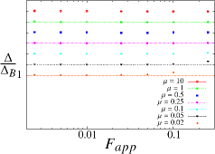
Figure 8: Full width at half height, $\Delta$, of the stress profiles, for a range of applied force perturbations and friction coefficients, when a single-peak stress response is observed. $\Delta_{B}=1.113z$ is the theoretical result. For each friction coefficient, data is shifted by one unit for convenience. ($\mu=10$ at top descending in order to $\mu=0.02$ at bottom.) For $\mu=0.05$ and $F_{app}=0.25kd$ and $\mu=0.02$ and $F_{app}=0.1kd$, larger full widths of the profiles indicating a deviation from the theory. For $\mu=0.02$ and $F_{app}=0.25kd$, the profile is shown in Figure 4 and appears as a twin-peak profile.

To provide a more quantitative comparison between the different plots shown in Figure 3, as well as to present our results in a manner that is closer in spirit to similar data obtained from 2d experiments, we show one dimensional stress profiles in Figures 4, 5, and 7. These stress profiles are obtained by circularly averaging the ‘bottom’ stress maps. Figure 4 shows the stress response profile, $\sigma$, at the bottom of the box for a relatively large, applied force $F_{\rm app}=0.25kd$, for packings with different friction coefficients. These profiles clearly indicate the role of friction in determining the nature of the stress response. Low friction results in a twin-peak profile of the anisotropic elastic variety, that transitions to a single-peak profile at larger friction corresponding to the isotropic, linear elastic Boussinesq theory Johnson (1987). These results are consistent with similar studies performed in two dimensional geometries Goldenberg and Goldhirsch (2005).

For a given friction coefficient the stress response is also sensitive to the magnitude of the perturbing force. We illustrate this point in Figure 5, where we show the stress profiles at the bottom of a packing with $\mu=0.01$, for different values of $F_{\rm app}$. Again, the common theme here is that the response changes character depending on $F_{\rm app}$. At smaller forces, there is little or no rearrangement in the particle contacts, and the underlying force network remains intact leading to a single peak profile. Whereas, for larger forces, a small fraction of contacts are broken, thereby causing the stresses to be propagated along better defined paths, leading to twin peak profiles. For the case where a single-peak response is obtained, we check that these profiles are consistent with isotropic, linear elastic theory, by fitting the profiles to the Boussinesq equation, Eq. 2 as shown in Figure 7, and extract the full width at half height. We note that there are no free parameters in this fitting procedure as the applied forcing is given as an input. As shown in Figure 8, we display our analysis as the ratio of the fitting to the expected theoretical result. Thus we confirm that the systems studied here do behave as an isotropic, elastic continuous medium over a range of parameters in friction and applied forcing.

To gain better insight into this transitional stress response we show the stress profiles in the plane parallel to the direction of the initial perturbation in Figure 6. These two-dimensional plots were obtained by spherically averaging the stress response about the location of the perturbation point. This view more clearly demonstrates how an initial anisotropic response - characterised by the twin-peak stress profile - transitions towards one with more traditional isotropic features - characterised by single lobe response profile - and ultimately how the extent of the force perturbation is eventually, in some sense, dissipated into the background stress. Closer inspection of the stress response, as visualised in Figure 3, reveals that anisotropic response features can extend arbitrarily far into the packing depending on the packing parameters.

IV.3 Response Scaling

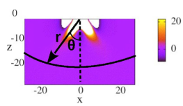
Figure 9: Scanning the circularly average stress response over angle $\theta$ at radial slices $r$, to identify the direction of the anisotropic response profile relative to the direction for the isotropic case (dashed line).

To characterise the transition between anisotropic and isotropic elastic stress response behaviours we designed the following procedure that identified how the maximum stress transmitted through the system deviated from traditional isotropic behaviour. For an isotropic, linear elastic continuum described by the Boussinesq equation, the maximum stress occurs in a line directly “below”, the point of force perturbation. Our circularly averaged stress analysis allows us to scan over angle $\theta$, to identify the direction of maximal stress transmission and monitor this response out to a radial distance, $r$, from the perturbation source. This construct is shown in Figure 9.

The anisotropic stress response in our $3D$ geometry transmits through a cone-like structure. Utilising the azimuthal symmetry of this geometry we angularly average the stress response, over angular elements $\Delta\theta=4^{\circ}$, leading to a $2D$ projection of the result as shown in Figure 10. The two vertical lines in Figure 10 provides us with a precise measure of the direction of maximum stress response relative to the direction for the expected isotropic maximum stress direction ($\theta=0$). We define the angular direction $\theta_{\mu}$ of maximal stress response as the average of these two peak locations.

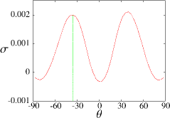
Figure 10: Circularly averaged stress profile, $\sigma$, for a system exhibiting an anisotropic, twin-peak profile ($F_{\rm app}=0.25kd$ and $\mu=0.05$). The profile peaks, identified with vertical lines, indicate the directions of the maximal stress and are denoted $\theta_{\mu}$ in the text.

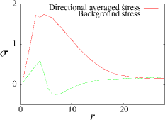
Figure 11: The circularly averaged stress response profile $\sigma$, in the direction $\theta_{\mu}$ of maximal stress (red solid line) and the background stress (green dashed line) in the direction $\theta=0$, identified in Figure 9 (for, $F_{\rm app}=0.25kd$ and $\mu=0.05$). This representative dataset shows how the characteristic length scale, $\xi_{\mu}$, at which the directional stress crosses the background stress is identified by the vertical line.

To identify a length scale that quantifies the nature of the mechanical state we measure the distance, $r$, from the origin of the localised force, in the direction of maximal stress, until that value of the stress is subsumed into the background stress. Starting from the angular slice closest to the perturbation source we scan elemental layers, layer-by-layer, away from the source to track the direction of the maximum stress. At each layer we compare the value of the stress in this direction $\theta_{\mu}$ with the stress in the same radial layer in the direction below the perturbing source, $\theta=0$. Thus, we define the characteristic length scale $\xi_{\mu}$ as the distance at which these two stress values become indistinguishable, as indicated by the vertical line in Figure 11.

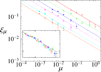
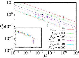
Figure 12: Influence of friction and force magnitude on the transition between isotropic and anisotropic stress response. (Left) Length scale $\xi_{\mu}$ characterising the distance from the location of the perturbing force at which the response crosses over from anisotropic to isotropic. The lines are power-law fits: $\xi_{\mu}\sim\mu^{-\alpha}$, with $\alpha=0.5\pm 0.06$. The scaled length data points are collapsed onto the line in inset. (Right) Angle direction of the anisotropic stress transmission relative to the central, isotropic direction. The lines are power-law fits: $\theta_{\mu}\sim\mu^{-\beta}$ for $\mu>0$, with $\beta=0.37\pm 0.07$. The scaled angles apart from uppermost data points are collapsed onto the line in inset. In both panels, the quoted force perturbations are in units of $kd$.

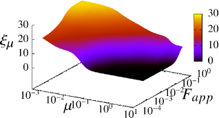
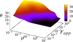
Figure 13: Phase diagrams of force perturbations, in applied force $F_{\rm app}$, and friction coefficient $\mu$, for the (a) $\xi_{\mu}$, and (b) stress transmission direction $\theta$. These $3D$ plots delineate between regions of isotropic, single-peak response (above) and anisotropic, twin-peak, response (below the dividing surface).

For the extensive parameter space in $\mu$ and $F_{app}$ explored here, we find that both the characteristic length scale $\xi_{\mu}$, and angle $\theta_{\mu}$, exhibit power law dependence on friction coefficient of the form

$$\xi_{\mu}\propto\mu^{-\alpha}$$ (6)

$$\theta_{\mu}\propto\mu^{-\beta}\text{\hskip 18.06749pt for $\mu>0$}$$ (7)

with the power-law exponents, $\alpha=0.5\pm 0.06$ and $\beta=0.37\pm 0.07$, over the range of friction and force magnitudes studied. Thus, the anisotropic-isotropic transition for stress response of a granular array is characterised by critical-like features accompanied by a length scale that grows as friction decreases. A subset of the data (for visual clarity) is presented in Figure 12. The very presence of a diverging length scale that distinguishes between different mechanical phases suggests that the anisotropic-isotropic transition for stress response of a granular array is characterised by critical-like features that are controlled by the friction coefficient. Curiously, this behaviour mimics the manner in which a thermodynamic system behaves in the vicinity of a continuous phase transition where now the friction coefficient plays the role of a reduced temperature. In this sense, the length scale defined here measures the spatial range of fluctuations in the stress over and above the background isotropic stress. Thus, to some extent the anisotropic-isotropic transition resembles a one-dimensional Ising model, where the zero-friction limit corresponds to the ordered phase and infinite friction is the analogue of the disordered phase, stable fixed point. For any friction ‘perturbations’, the response is readily driven away from the zero-friction, anisotropic phase, and always ends up exhibiting isotropic stress response for large enough system size.

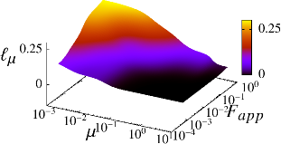
Figure 14: Three dimensional phase diagram, in the space of applied force $F_{app}$ and particle friction coefficient $\mu$, for the anisotropic-isotropic transition of mechanical response within a granular array, parameterised by the effective length scale, $\ell_{\mu}\equiv\xi_{\mu}\sin\theta$ where $\xi_{\mu}$ is normalised by simulation box size.

Upon collating the data over our entire parameter space: $\mu=\{0,10.0\}$ and $F_{\rm app}=\{0.0005,0.25\}$, we are able to map the stress response behaviour onto the pseudo-phase diagrams shown in Figure 13. These diagrams delineate regions of parameter space where an anisotropic response is expected (region below the boundary) and those parameters which are more likely to result in an isotropic, linear elastic response (above boundary). Anisotropic behaviour emerges for low friction and high forcing where the stress peaks extend far into the packing and are directed away from perturbation direction. It is only in the $\mu=0$ limit that the anisotropic length scale spans the simulation domain. Conversely, isotropic character is recovered for mildly frictional materials and moderate forcing.

Combining these two plots we present the anisotropic-isotropic transition in stress response as parameterised by the effective length scale, $\ell_{\mu}\equiv\xi_{\mu}\sin\theta$, where $\xi_{\mu}$ is normalised by the simulation box size, in Figure 14. The boundary distinguishes between the stress state within a single system. For points below the boundary, the granular medium behaves as an anisotropic, elastic material, where stresses are transmitted through the system along directed pathways commensurate with the structure of the packing. Above the boundary, the material will resort to behaviour more consistent with an isotropic, elastic solid. Thus, small systems subject to relatively large forces will appear to behave as anisotropic materials that may result in failure along the directions of the largest stress propagation. Whereas large frictional aggregates can be considered, as is well-known from everyday experience tells us, as isotropic elastic media.

V Conclusions

Large-scale computer simulations of overcompressed FCC granular arrays over a wider range in friction coefficient and point force perturbations were carried out to study the stress response inside these arrays. Our results indicate that packings with large particle friction subject to small localised forcings, exhibit a single lobe stress response consistent with classical, isotropic elasticity. Whereas, packings with low friction and subject to large localised force magnitudes exhibit ring-like stress responses, a hallmark of anisotropic elastic behaviour. However, this anisotropic state diminishes with distance from the perturbation source, within the same packing, and transitions towards a more elastic-like character at a length scale that depends on the friction coefficient. This characteristic length scale grows with decreasing friction. Ultimately, the limit of purely frictionless packings appear to present as a pathological case in this problem - showing anisotropic behaviour out to the largest distances. Any non-zero friction will ultimately send the system towards an isotropic elastic regime in the thermodynamic limit.

While the FCC arrays used in this study clearly enhance the possibility of observing strongly anisotropic behaviour, the presence of disorder is likely to suppress such features Goldenberg and Goldhirsch (2005); Silbert (2010a, a). Thus, we expect that a combination of varying structural disorder and friction provide the necessary ingredients for packings that can be constructed with tailored mechanical properties. It might also be that as a disordered granular system is brought closer to its point of marginal rigidity, it may become increasingly fragile Cates et al. (1998); Kasahara and Nakanishi (2004), and remain as an anisotropic medium at all friction values, thus providing a broad range of possible mechanical states to choose from.