Abstract

The effects of interpersonal interactions on individual’s agreements result in a social aggregation process which is reflected in the formation of collective states, as for instance, groups of individuals with a similar opinion about a given issue. This field, which has been a longstanding concern of sociologists and psychologists, has been extended into an area of experimental social psychology, and even has attracted the attention of physicists and mathematicians. In this article, we present a novel model of opinion formation in which agents may either have a strict preference for a choice, or be undecided. The opinion shift emerges during interpersonal communications, as a consequence of a cumulative process of conviction for one of the two extremes opinions through repeated interactions. There are two main ingredients which play key roles in determining the steady state: the initial fraction of undecided agents and the conviction’s sensitivity in each interaction. As a function of these two parameters, the model presents a wide range of possible solutions, as for instance, consensus of each opinion, bi-polarisation or convergence of undecided individuals. We found that a minimum fraction of undecided agents is crucial not only for reaching consensus of a given opinion, but also to determine a dominant opinion in a polarised situation. In order to gain a deeper comprehension of the dynamics, we also present the theoretical master equations of the model.

Introduction

When a group of inter-related individuals discuss around a given item, they are feasible to change their initial opinions in order to get closer to or farther from other subjects in the group. This interpersonal dynamics leads to different collective behaviours which could be categorised either by consensus or coexistence of opinions. If furthermore the topic is a binary statement, as for example a pro-against issue, the coexistence of opinions turns out to be a polarised state, where a fraction of the group holds a given opinion and the rest the opposite one.

These kind of situations lead naturally to questions like: Which are the mechanisms underlying the formation of these collective states? or, can we predict the final collective outcomes when different mechanisms compete among them, as for instance if some individuals tend to agree and others tend to disagree?

A numerical modelling approach could be a powerful tool in order to face these kind of questions and test how a given interaction mechanism between pair of agents lead to the formation of collective states. The typical approach to model opinion formation is to assume that an individual either adopts the opinion of a neighbour or decides on an opinion based on the average of neighbouring opinions. We take a different conjecture, that the process of opinion formation is an emergent behaviour of an underlying dynamics. Here, we develop a novel mathematical model based on the combination of interaction-based conviction accumulating dynamics and a threshold-driven opinion change.

In sociological research, the concept of threshold was stated in the seminal papers of T. Schelling [31] and M. Granovetter [17] in order to understand the micro-macro link and the aggregation processes. From the psychological perspective, accumulative-threshold models have been successfully used [34, 33] in order to understand binary decision making problems.

The formation of opinion’s collective states and the underlying mechanism has largely studied from sociology and social psychology [11, 20, 19, 1, 4] among others. There are five main theories to explain group opinion dynamics [12, 10]: Social comparison theory [11, 3, 30]; Information or Persuasive arguments theory (PAT) [39, 26]; Self-categorization theory [37, 28, 27]; Social decision theory [7, 21, 18] and Social influence network theory [12]. Predominantly, these theories are focused on interpersonal interactions, and it is useful because it draws attention to the emergent communication patterns. Essentially, it deepens the understanding of group dynamics, in particular when combined with an appropriate mathematical model.

From a theoretical point of view, much of the existing modelling development about opinion dynamics has been addressed from a physics-based framework, where the behavioural mechanism of social influence are derived from analogies with physical systems, in particular spins [6, 23]. The variety of existing models assume that individuals hold binary or continuous opinion values (usually lying between -1 and 1), which are updated over repeated interactions among neighbouring agents. Different models assume different rules of opinion adaptation, such as imitation [1], averaging over individuals with similar opinions [40], the majority rule[13], or more sophisticated rules [25, 36]. The classical models that are based on the mechanisms of convergence (after interacting, individuals get more similar) predict consensus. The models which include mechanism of negative influence (disliking of dissimilar ones) naturally will give place to bi-polarisation. However, in last years new models with interesting features appeared, as for instance, a model of continuous opinion based on persuasive arguments theory [24] where bi-polarisation can been produced without including negative influence explicitly. Another model presented in [22], explores the competition between the two antagonist mechanisms, as persuasion and compromise, among agents with different degree of agreement about a given issue.

In this work we present an agent-based model for a population of interdependent individuals who simultaneously participate in an artificial interaction process. The individuals can have two opposing views, and also a third state of indefiniteness. Through the interactions, individuals with opinions drive the undecided ones towards one of the definite opinions and also undecided agents can wear down the conviction of decided ones. This gives place to a random cumulative process where individuals can eventually change their convictions about the issue in question [22, 35] and, when this conviction overpasses a certain threshold, the opinion changes. Thus, the opinion dynamics is an emerging process depending of the underlying evolution of the conviction of each individual about a given issue. We are mainly interested in the equilibria reached by this population. We analyse the convergence properties of the system for wide range of parameter’s values and found that three main collective states can be seen: bi-polarisation, consensus and convergence of undecided agents. Moreover, the model shows that the initial fraction of undecided agents could be crucial in the determination of consensus or the dominance of a given opinion in a polarised situation. We also analyse how the model can achieve the mentioned collective states in a regime of initially low concentration of undecided individuals and finally we sketch the exact dynamical equations in order to frame the model within the non-linear and non-local first order differential equation formulation.

The article is organised as follows: the model and the interaction dynamics are presented in section Analysis. The results are presented and discussed in section Results. We conclude in section Discussion.

Analysis

In order to study the opinion formation process in groups of interrelated people we develop a simple agent-based model that includes the main relevant features for modelling the opinion dynamics: convergence (in subsequent interactions individuals get to similar others) and negative influence (disliking of dissimilar others).

We consider a population of $N$ individuals $(i=1,2,\dots,N)$, each one simultaneously participating in interpersonal communication process, which can be understood as an exchange of some kind of information between two or more agents over the issue in question. The population has the following characteristics: each individual is represented as an agent $i$, with a numerically valued opinion $O(i)$ which stands for agent’s posture on a given issue at period $t$. The opinion variable $O(i)$ can take three values of attitude towards an issue: positive $O(i)=+1$, negative $O(i)=-1$, and neutral $O(i)=0$.

In addition, the agent $i$ has a conviction about the issue in question, represented by a variable $C(i)$. This conviction variable $C(i)$ could vary between $C_{max}$ and $-C_{max}$, and represents being fully aligned with the interaction communication or totally opposed with it.

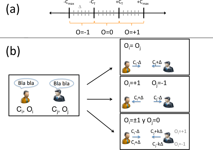
Figure 1: Schematic representation of the opinion dynamics. Panel (a): Relation between conviction ($C$) and opinion ($O$). Each conviction interval ($[-C_{max,C-_{T}}],[-C_{T},C_{T}],[C_{T},C_{max}]$) defines one of the three opinion values ($O=-1,0,+1$ respectively). Moreover, each interval is divided in sub-intervals of length $\Delta$. For our simulations we choose $C_{T}=1$ and $|C_{max}|=3$ (in Figure 5 $C_{T}$ takes other values also) such as all conviction interval has the same length. Panel (b): Description of how conviction is modified by the pairwise interaction dynamics for three different cases: Same opinion (top panel), opposite opinions (middle panel) and defined opinion vs undecided.

These two variables are not independent, i.e., if the conviction variable $C(i)$ is greater than a given positive threshold, $C(i)>C_{T}$, the agent has a positive opinion $O(i)=+1$, and if it is less than a given negative threshold, $C(i)<-C_{T}$, the agent’s opinion is negative $O(i)=-1$. If the conviction held by the agent does not allow him to decide with any definite position, then the agent is undecided and $O(i)=0$ (see Figure 1 (a)).

Dynamics

We are interested in the equilibria reached by the system when agents meet and interact in successive periods. We model this as a process where agents may increase or decrease their convictions depending on whether the opponent in each discussion has positive or negative opinion. These social interactions produce cumulative changes that can eventually lead to the change of opinion: a shift in opinion occurs when that conviction exceeds a certain threshold.

The interaction dynamics between agents is the following: whenever two agents $i$ and $j$ interact, the agents’ conviction values $C(i)$ and $C(j)$ are modified by an amount bounded by $k\Delta$, depending on the opinion of both individuals. This parameter, $\Delta$, is a measure of the sensitivity of the agents to a given interaction.

This social influence mechanism acts as by moving the respective convictions from their existing positions towards new ones depending of the interacting opponent. This way the opinion shift is not based on the imitation of opinions of the neighbours (like the typical imitation behaviours), but is due to a cumulative process of conviction for one of the two extremes opinions, after repeated interactions.

The presence of the two social ingredients of the interacting dynamics, convergence and negative influence, will produce an “anti-flocking effect”: Distant individuals repel (caused by mechanism of negative influence) if they differ in opinions and get attracted by each other if their opinions are similar (mechanism of convergence and social influence). This last is in line with the fact observed by Wood [42] where individuals sharing a common attribute tend to get closer in opinions.

More formally, at each period $t$, the states of the agents after interaction are updated according to the following rules, also illustrated in Figure 1 (b) :

• If agents share the same opinions, $O_{i}(t)=O_{j}(t)$, and $C_{i}(t)>C_{j}(t)$ then they get attracted (agents influence each other so that their convictions become more similar)

  $$C_{i}(t)=C_{i}(t)-\Delta,$$

  $$C_{j}(t)=C_{j}(t)+\Delta.$$

• If agents hold different opinions, $O_{i}(t)=+1$, and $O_{j}(t)=-1$ then they repel

  $$C_{i}(t)=C_{i}(t)+\Delta,$$

  $$C_{j}(t)=C_{j}(t)-\Delta.$$

  If one of the agents has an opinion and another one is undecided, then they get attracted. In this case the dynamics is asymmetric simulating the fact that is not the same convincing someone who does not have any opinion yet or making someone change his opinion:

• If $O_{i}=-1$ and $O_{j}=0$ then

  $$C_{i}(t)=C_{i}(t)+\Delta,$$

  $$C_{j}(t)=C_{j}(t)-k\Delta.$$

• If $O_{i}=+1$ and $O_{j}=0$ then

  $$C_{i}(t)=C_{i}(t)-\Delta,$$

  $$C_{j}(t)=C_{j}(t)+k\Delta.$$

In the way the rules are actually written, some anomalous behaviour can arise for large values of $\Delta$. For instance, if two agents have very similar convictions, they should be attracted. But if $\Delta$ is larger than the difference of their convictions, it would happen that after the interaction they will be more distant in their convictions. In order to avoid these kind of undesirable behaviours, we set $\Delta_{eff}=\frac{|C(i)-C(j)|}{2}$ if $|C(i)-C(j)|<\Delta$.

The main parameters of the model are:

• $\Delta$ is a sensitivity parameter which measures how much the conviction of an agent changes after each interaction. The smaller it is, the more agents who share the same opinion are needed to convince him.

• $P_{0}$ is the initial fraction of undecided agents.

• $C_{T}$ is the threshold beyond which the agent is no longer undecided and adopts an opinion.

• $k$ is a variable which simulates an asymmetry dynamics between an undecided agent and the one with a formed opinion. Values $k>1$ imply that the conviction’s change of the undecided is modified by a factor $k$ with respect to the other one.

Given the details of the interaction dynamics we are interested in the following question: Do the interactions among the agents with different opinions bring the group to consensus o bi-polarisation?

We present the results of simulations in the next sections. All the simulations are done for systems with $N=1000$ agents. Results are averages over ensembles $N_{ev}=1000$ equivalent configurations, corresponding to different realisations of the random initial conditions.

Results

In this section we present the steady states of the model and discuss its properties as a function of the relevant parameters. The aggregate behaviour is characterised in terms of the fraction of agents who state an opinion $i$, $S_{i}$, where $i=\{+,-,0\}$. Given that $S_{i}(t)$ is a function of time, we call $P_{i}\equiv S_{i}(0)$ the initial fraction of agents who has an opinion $i$, and $T_{i}\equiv S_{i}(t_{asint})$ the fraction of agents who have come to a definite position on an issue or have ”no opinion” at convergence.

There are two features of the model that, a priory, are preferred to be fixed: first, opinions should be equally likely; second, it is assumed to be easier for agents who are undecided to adopt a particular opinion because they have got persuaded, than for those who have an opinion to turn into ”undecided”. The first one is implemented in a way that once the initial fraction of undecided agents, $P_{0}$, is chosen, the rest of the agents are equally distributed with both opinions ($\pm 1$). When we change this condition, we will call $P_{+}$ the fraction of agents with $O=+1$ after the undecided are assigned. The second one is achieved by setting $k=2$. The conviction of each agent is chosen at random from an uniform distribution within each opinion.

For better description and interpreting interaction effects is especially useful to take in Figure 1.

Equilibrium States

We start with analysing the steady states $T_{i}\equiv S_{i}(t_{asint})$ as a function of $P_{0}$ and $\Delta$. We vary them $0.01\leq P_{0}\leq 0.99$ and $0.01\leq\Delta\leq 1.0$ with steps of $0.01$ . Results are obtained with asynchronous updating where the procedure is iterated until convergence.

As a result of simulations, the system converges to one of these four equilibrium states:

(a)

All undecided agents ($O_{i}=0$ $\forall i$).

(b)

Positive Consensus ($O_{i}=+1$ $\forall i$).

(c)

Negative Consensus ($O_{i}=-1$ $\forall i$).

(d)

Bi-Polarisation (fractions of agents having $O=+1$ and $O=-1$).

The steady state is reached when $T_{0}=1$ or $T_{0}=0$, i.e. agents are either all undecided or all have an opinion. Given the constraint $S_{0}(t)+S_{+}(t)+S_{-}(t)=1$ ($\forall t$), if $T_{0}=0$, the only possible equilibria are either consensus of one of the extreme opinion (b-c) or bi-polarisation (d).

If we look at the system in terms of the fraction of undecided agents, there is a transition from $T_{0}=1$ to $T_{0}=0$ (i.e. there are no longer agents who have ”no opinion”). This transition depends on the value of $P_{0}$ and $\Delta$. This result is due to a nonlinear nature of the underlying opinion forming dynamics, and is different to what is observed in a reference paper [38]. The authors examined a three-state generalisation of the voter model where two states (”rightists” and ”leftists”) are incompatible and interact with a third state (”centrists”) to impose their consensus. In this case the dynamics can settle in a polarised state consisting only of leftists and rightists.

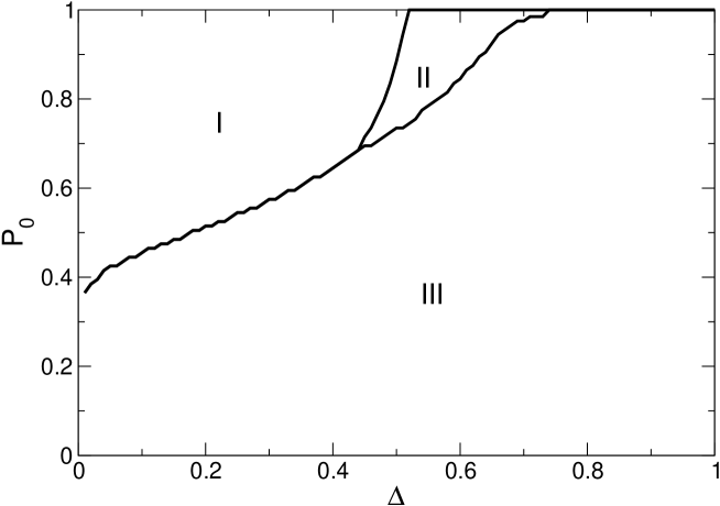
Figure 2: Fundamental Phase Diagram: Dominant steady state solution as a function of $P_{0}$ and $\Delta$. We identify three different regions: Region I, convergence of undecided; Region II, consensus of opinions +1/-1 and Region III, bi-polarisation. In the simulations $C_{T}=1$, $k=2$, $C_{max}=3$ were used.

Figure 2 shows the Fundamental Phase Diagram ($FPD$) that depicts existence of different regions of the system under equilibrium. In this Phase Diagram we analyse the prevalence of each equilibria for every pair of values of $P_{0}$ and $\Delta$ within the specific range. Be $\langle T_{i}\rangle$ ($i=\{+,-,0\}$) the ensamble average of $T_{i}$, the larger value of $\langle T_{i}\rangle$ will determine the dominant solution.

The Phase Diagram exhibits three different regions (see Figure 2):

Region $I$,

delimited by large values of $P_{0}$ and small values of $\Delta$, where the equilibrium state is characterised by the convergence of undecided agents (i.e. $O=0$ $\forall i$).

Region $II$,

delimited by large values of $P_{0}$ and intermediate values of $\Delta$, where the equilibrium state is characterised by the consensus of one of the extreme opinions ($O=+1$ or $O=-1$). This is the most unusual result because it is accompanied with the implicit symmetry breaking in this region.

Region $III$,

delimited by low values of $P_{0}$ when $\Delta$ is small and by all values of $P_{0}$ when $\Delta$ is large, where the steady state is defined by a bi-polarisation of opinion, i.e. fractions of agents having $O=+1$ and $O=-1$.

Figure 1 can be used again to illustrate a bit more intuitively how agents interact through this model. When a pair of facing individuals interact, there are two mechanisms that take place: the first trying to gather together those who share the same opinion, and the second that makes agents change opinions. For example, if both agents are undecided they will keep their positions and get closer in their convictions. If one is undecided and another has an opinion, both will modify their convictions, but the former will get more similar to the other one, which may eventually make him adopt a position. Due to this kind of repeated interactions these agents will eventually get closer to the thresholds $\{-C_{T},C_{T}\}$ (see Figure 1 (a)). On the other hand, if both have opinions they will not change them, but they will modify their convictions: either approaching them (if both share the same opinion) or dissociating them (if otherwise). Synthesising, there are exist two competing opposite forces: first, which drives agents to the center in the conviction space (turning them to ”undecided”), another which drives agents to its extremes, forcing bi-polarisation of opinions. The final result of mutual interactions depends on the initial fraction of undecided agents $P_{0}$, and the sensitivity parameter $\Delta$ (see Figure 2).

When $\Delta$ is small, the situation is dominated by agents that change convictions very little after pairwise interactions. Thus, many of these interpersonal relationships are needed in order to force a change in their opinions. Here, the fraction $P_{0}$ is important because it determines what will be the final state of this dynamics (all undecided ($\langle T_{0}\rangle=1$) or none ($\langle T_{0}\rangle=0$)).

Instead, when $\Delta$ increases, the preference for an agent to adopt extreme opinions (due to the asymmetry given by $k$, see Figure 1(b)) is more evident and is reflected in the fact that the more initially undecided agents are needed in order for the system to reach the final state with “all undecided”. As a consequence, the border of Region $I$ grows monotonically with $\Delta$ until enclosing with $P_{0}=1$. When $\Delta$ is large, the final state is bi-polarisation (Region $III$) independently of the initial density of undecided agents.

Consensus and Bi-Polarisation

Given a global picture of the stable solutions, we look in details at the dynamics which makes the systems reach these states. Furthermore, we restrict the discussion to Regions $II$ and $III$ where the equilibrium states are consensus and bi-polarisation, respectively, because Region $I$ does not represent any interest neither from the social nor the individual point of view .

Region $III$ deserves a closer look. On average, the distribution of $T_{+}$ and $T_{-}$ (the fraction of agents who have an opinion and the fraction of undecided agents at convergence, respectively) is $50\%-50\%$, and depends on $P_{0}$ and $\Delta$.

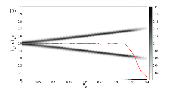
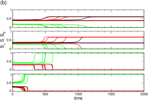
Figure 3: Bi-polarisation Region. Panel (a): Distribution of positive opinions ($T_{+}$) and its average ($<T_{+}>$) as a function of $P_{0}$ for $\Delta=0.01$. Panel (b): Fraction of agents with opinion $O=+1$ ($S_{+}(t)$, black), $O=-1$ ($S_{-}(t)$,red) and undecided ($S_{0}(t)$, green) as a function of time for different undecided initial concentration (From top to bottom: $P_{0}$=0.20, $P_{0}$=0.30, $P_{0}$=0.40, $P_{0}$=0.50).

On Figure 3 we plot the distribution of positive opinions, $T_{+}$, and its average, $\langle T_{+}\rangle$ as a function of $P_{0}$ for different values of $\Delta$. It can be observed that, as well as the dynamics is confined to Region $III$, the averaged value of positive opinion is fifty percent, i.e., $\langle T_{+}\rangle=0.5$. However, the behaviour of the distribution of positive (negative) opinion depends on $P_{0}$ and $\Delta$. For example, for $\Delta=0.01$, a clear bimodal distribution emerges (see Figure 3 (a)). It can be observed that the mean value of each branch depends linearly on $P_{0}$, either increasing or decreasing. This behaviour can be understood if we look at Figure 3(b), where the dynamics of the fraction of agents with a given opinion ($S_{i}$, $i=\{+,-,0\}$) is plotted against time for different values of $P_{0}$. Here it can be seen that as the system approaches the final state, almost total number of undecided agents adopts massively either one of the two opinions with the same probability. If for example, there are initially $20\%$ of undecided agents, it means that there are $40\%$ of agents with positive opinion and $40\%$ of agents with negative opinion. Due to the dynamics, the system will converge either to the state with $60\%$ ($T_{+}=0.60$) or $40\%$ with positive opinions ($T_{+}=0.40$). When $P_{0}=0.1$ the final states for $T_{+}$ will be $0.45$ or $0.55$, corresponding to closer values of the mean of the bimodal distribution. But if $P_{0}=0.30$ then $T_{+}$ will be $0.35$ or $0.65$ corresponding to the regions where the two branches are more distant from each other.

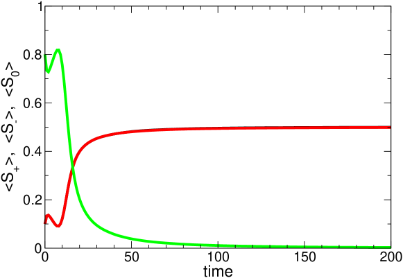
Figure 4: Averaged opinion dynamics in region II of the Fundamental Phase Diagram. The plot shows the averaged evolution in time for each opinion dynamics ($<S_{+}>$, black, $<S_{-}>$, red and $<S_{0}>$, green). It can be observed that undecided population grows until it reach a value above $80\%$ in the first time steps but finally one of the populations with defined opinions becomes dominant with the same probability. Evolutions are averaged over $N_{ev}=10000$. $P_{0}=0.80$, $\Delta=0.55$.

Region $II$ is the most interesting one, given that all agents adopt, equally likely, one of the two extreme opinions. This region expresses the range of parameter values where a given opinion prevails and it involves a symmetry breaking in the dynamics. In Figure 4 we plot the average opinion dynamics as a function of time for $P_{0}=0.80$ and $\Delta=0.55$. If we look at the fraction of undecided agents, it can be seen that after a slight decrease it reaches more than $80\%$ of the population, and then it decreases monotonically until disappears. When it happens, just one of the two opinion survives.

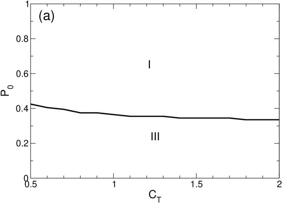
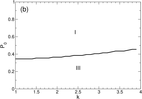
Figure 5: Alternative Phase Diagram. Panel (a): Regions of dominant solution as a function of $P_{0}$ and $C_{T}$ for $\Delta=0.01$. This plot shows that in the low $\Delta$ region and with symmetric distribution of opposite opinions, the systems evolves either to bi-polarisation or convergence of undecided, depending of the initial fraction of undecided individuals, as have been seen in the Fundamental Phase Diagram (Figure 2). Panel (b): Same plot for $P_{0}$ vs $k$ and $\Delta=0.01$. In both cases, the main difference of the Fundamental Phase Diagram is the dependence of the transition between Region I and III with $C_{T}$ and $k$ respectively, as it is explained in the main text.

We also explored the impact produced on the Fundamental Phase Diagram when the threshold $C_{T}$ and the asymmetry parameter $k$ are modified. Increasing the threshold makes the intermediate interval of the conviction space, which defines agents to be undecided, to be bigger. Less undecided are needed initially (at $t=0$) in order to have more of them at the end. This moves the transition $T_{0}=0\to T_{0}=1$ down (see Figure 5 (a)). This in turn, results in the final disappearance of Region $II$, which produces that Region $I$ becomes dominant in the phase space. Decreasing the threshold produces the opposite effect: the polarisation Region $III$ becomes bigger.

Instead, with increasing k, grows the tendency to adopt a definite opinion ($+/-1$) after each interaction, and therefore, more undecided individuals are needed in order to achieve a final state where they predominate. Thus, this moves the transition up (see Figure 5 (b)). When the asymmetry parameter is changed, the model moves between a pragmatic null ”symmetric” model ($k=1$) and a more extreme asymmetric case ($k>2$). With large $k$, the polarization region becomes dominant.

How many undecided are relevant?

In real social situations, the value of $P_{0}$ depends on the underlying context, and it may be large or small. Clearly, if we consider examples of voting elections, then assuming very large values of $P_{0}$ is less feasible. It is hard to imagine a social system where there is a huge percentage of undecided voters. In fact, voting must be considered carefully because the term “undecide” requires correct precision according to Gordon [16], and Galdi [14].

Instead, social examples of college decision (up to $50\%$ of students enter college as “undecide” [16]) or the choice of major (an estimated $75\%$ of students change their major at least once before graduation [16]) present situations where large values of $P_{0}$ are justified.

In the previous section we showed that, for small values of $\Delta$, when the initial fraction of undecided agents, $P_{0}$ is large, the system presents three solutions, and when $P_{0}$ is small the equilibrium is bi-polarisation. Thus, we are interested in the next question: in systems with a relatively small fraction $P_{0}$ what should be undertaken in order to obtain the equilibria states observed previously.

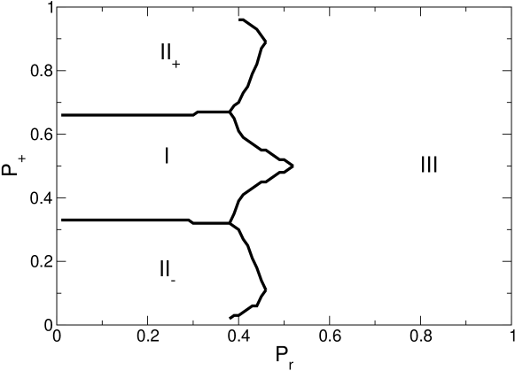
Figure 6: Another Alternative Phase Diagram. Regions of dominant solution as a function of $P_{+}$ (Bias) and $P_{r}$ (Repulsion probability) for initially low undecided concentration and small $\Delta$ ($P_{0}=0.10$ and $\Delta=0.01$). If $P_{r}=1$, individuals with opposite opinions always repel and the steady state is a polarised situation as we found in the Phase Diagram of Figure 2. When $P_{r}<1$, it can happen that agents with opposite opinions get attracted and the steady state depends on the bias to some opinion. If some of the opinion initially prevails, then the population will go to the consensus of this opinion. Otherwise, a convergence of undecided agents for $P_{r}<0.40$ approx. is reached.

We propose an alternative scenario for the interaction dynamics. Instead of implemented repulsive effect, allow the individuals with opposite opinions repel with some positive probability $P_{r}$, in a similar way it was treated in [22]. The concentration of undecided is fixed. The Phase Diagram for $P_{+}$ vs $P_{r}$ (Repulsion probability) for initially low concentration of undecided agents and a small value of $\Delta$ ($P_{0}=0.10$ and $\Delta=0.01$) is presented in Figure 6.

When $P_{r}=1$, agents with opposite opinions always repel and the equilibrium is a polarised state found in the Phase Diagram on Figure 2. When $P_{r}<1$, agents sharing opposite opinions may get attracted with probability $(1-P_{r})$, and the steady state depends on the bias to any opinion. If any of the opinion initially prevails, then the population will reach the consensus to this opinion. Otherwise, a convergence to “all undecided” for $P_{r}<0.40$ approx. is reached.

The two scenarios for the interaction dynamics analysed here are interesting from the social point of view because, in turn, they correspond to the two different sides of the public debate: “Do we learn more from the people with opposite opinions of our own?”. On one side there is a view that we learn much more from people with similar opinions because we do learn more arguments fortifying that belief and take things as facts. On the other side, there is a view that we only learn if we look beyond: in a discussion with people with opposing thoughts we see the different points of view, the exchange of thoughts, etc.

Theoretical Approach

In order to gain a deeper comprehension of the dynamics of this model, we present in this section the master equations corresponding to the dynamics of the systems. We look at the system as composed by three populations, according the opinions of the agents. Lets recall than an agent with opinion $O=+1$ has a conviction $C\in[C_{T},C_{max}]$, another with $O=0$ has $C\in[C_{T},-C_{T}]$ and an individual with $O=-1$ has $C\in[-C_{max},-C_{T}]$. We divide the interval corresponding to each opinion in $M=\Delta^{-1}$ subintervals. Given the evolution of the conviction according to the interaction-evolution rules detailed in previous sections, the best way to describe the dynamics of the model is in terms of the density of agents with a given conviction. With this goal we define this density for $1\leq j\leq M$ and $t\geq 0$,

$$s_{+}(j,t)=\frac{\#\{i\in[C_{T}+(j-1)\Delta,C_{T}+j\Delta)\}}{N},$$

$$s_{0}(j,t)=\frac{\#\{i\in[-C_{T}+(j-1)\Delta,-C_{T}+j\Delta)\}}{N},$$

$$s_{-}(j,t)=\frac{\#\{i\in[-C_{T}-(j-1)\Delta,-C_{T}-j\Delta)\}}{N},$$

which represent the fraction of agent of each opinion with conviction in each interval of length $\Delta$. In this way we can obtain a coupled system of $3M$ difference equations governing the evolution of the density of agents.

We call $S_{i}^{k\leq j}(t)=\sum_{k=1}^{j}s_{i}(j,t)$, $S_{i}^{k\geq j}(t)=\sum_{k=j}^{M}s_{i}(j,t)$, and recall that $S_{i}(t)$ is the fraction of agents with opinion $i$, where $i\in\{+,-,0\}$.

In the following, we omit the variable $t$ in the right hand side of the equations for brevity. After some characteristic time $\tau$, depending on the rate of the interactions, we have that the variation on the density of agents is given by the balance between gain and loss terms. For example, when $O=-1$, we have

$$s_{-}(j,t+\tau)-s_{-}(j,t)=G_{-}(j,t)-L_{-}(j,t)$$

where the term $G_{-}$ corresponds to those agents located at $j-1$ which interact with an agent with opinion $O=+1$ or an agent with opinion $O=-1$ and a stronger conviction, plus those agents located at $j+1$ which interact with an agent with neutral opinion $O=0$ or an agent with opinion $O=-1$ and a weaker conviction:

$$G_{-}(j,t)=2s_{-}(j-1)[S_{+}+S_{-}^{k\geq j}]+2s_{-}(j+1)[S_{0}+S_{-}^{k\leq j}].$$

On the other hand, the loss term corresponds to interactions between an agent located at $j$ with another agent in any other location,

$$L_{-}(j,t)=-2s_{-}(j)[1-s_{-}(j)].$$

So, in this way we obtain the following system of equations:

$$\begin{array}[]{rl}s_{-}(j,t+\tau)-s_{-}(j,t)=&-2s_{-}(j)[1-s_{-}(j)]+2s_{-}(j-1)[S_{+}+S_{-}^{k\geq j}]\\ &+2s_{-}(j+1)[S_{0}+S_{-}^{k\leq j}],\\ s_{+}(j,t+\tau)-s_{+}(j,t)=&-2s_{+}(j)[1-s_{+}(j)]+2s_{-}(j-1)[S_{-}+S_{+}^{k\geq j}]\\ &+2s_{+}(j+1)[S_{0}+S_{+}^{k\leq j}],\\ s_{0}(j,t+\tau)-s_{0}(j,t)=&-2s_{0}(j)[1-s_{0}(j)]+2s_{0}(j-1)S_{+}^{k\geq j}+2s_{0}(j+1)S_{+}^{k\leq j}\\ &+2s_{0}(j+k)S_{-}+2s_{0}(j-k)S_{+}\\ \end{array}$$

for $2<j<M$.

For $j=1,2$ and $M$, the equations are slightly different, as for instance can be seen for $s_{-}$:

$$\begin{array}[]{rl}s_{-}(1,t+\tau)-s_{-}(1,t)=&-2s_{-}(1)[1-s_{-}(1)]+2s_{0}(2)S_{-}\\ &+2s_{-}(2)[S_{0}+S_{-}^{k\leq 1}],\\ s_{-}(2,t+\tau)-s_{-}(2,t)=&-2s_{-}(2)[1-s_{-}(2)]+2s_{-}(1)[S_{+}+S_{-}^{k\geq 2}]\\ &+2s_{-}(j+1)[S_{0}+S_{-}^{k\leq j}]+2s_{0}(1)S_{-},\\ s_{-}(M,t+\tau)-s_{-}(M,t)=&-2s_{-}(M)[1-s_{-}(M)]+2s_{-}(M-1)[S_{+}+s_{-}(M)],\\ \\ \end{array}$$

Up to here, we can see that the equations are rather difficult to study, but we can gain more perspective if we move from this discrete version to a continuous model. We can do that by introducing (smooth) functions $u_{i}(x,t)$, $i\in\{0,+,-\}$, defined for $(x,t)\in[0,1]\times[0,\infty)$ such that

$$u_{i}(j\Delta,t)=s_{i}(j,t),$$

and we can approximate the spatial partial derivative as

$$\Delta\partial_{x}u_{i}(j\Delta,t)\approx s_{i}(j+1,t)-s_{i}(j,t)\approx s_{i}(j,t)-s_{i}(j-1,t),$$ (1)

and the temporal partial derivative as

$$\tau\partial_{t}u_{i}(j\Delta,t)\approx s_{i}(j,t+\tau)-s_{i}(j,t).$$

Also,

$$S_{i}^{k\geq j}(t)\approx\int_{0}^{j\Delta}u_{i}(y,t)dy,\qquad S_{i}^{k\leq j}(t)\approx\int_{j\Delta}^{1}u_{i}(y,t)dy,$$

We assume that $\tau=\Delta$, which corresponds to a time scaling of the rate of interactions.

After some algebra, the continuous version of the master equations reads as

$$\frac{1}{2}\partial_{t}u_{-}(x,t)= \partial_{x}\Big{[}u_{-}(x,t)\Big{(}\int_{0}^{x}u_{-}(y,t)dy-\int_{x}^{1}u_{-}(y,t)dy\Big{)}\Big{]}$$

$$+\partial_{x}\Big{[}u_{-}(x,t)\Big{(}\int_{0}^{1}u_{0}(y,t)dy-\int_{0}^{1}u_{+}(y,t)dy\Big{)},$$

$$\frac{1}{2}\partial_{t}u_{+}(x,t)= \partial_{x}\Big{[}u_{+}(x,t)\Big{(}\int_{0}^{x}u_{+}(y,t)dy-\int_{x}^{1}u_{+}(y,t)dy\Big{)}\Big{]}$$

$$+\partial_{x}\Big{[}u_{+}(x,t)\Big{(}\int_{0}^{1}u_{0}(y,t)dy-\int_{0}^{1}u_{+}(y,t)dy\Big{)},$$

$$\frac{1}{2}\partial_{t}u_{0}(x,t)= \partial_{x}\Big{[}u_{0}(x,t)\Big{(}\int_{0}^{x}u_{0}(y,t)dy-\int_{x}^{1}u_{0}(y,t)dy\Big{)}\Big{]}$$

$$+2\partial_{x}\Big{[}u_{-}(x,t)\Big{(}\int_{0}^{1}u_{0}(y,t)dy-\int_{0}^{1}u_{+}(y,t)dy\Big{)}.$$

The boundary conditions for $s_{-}$ are given by

$$u_{-}(0,t)= \Big{(}\frac{\int_{0}^{1}u_{-}(y,t)dy}{\int_{0}^{1}u_{-}(y,t)dy+\int_{0}^{1}u_{+}(y,t)dy}\Big{)}2u_{0}(0,t),$$

$$\partial_{x}u_{-}(M,t)= 0,$$

and the ones corresponding to $u_{+}$ are similar. The no flux boundary condition at $x=1$ follows from the assumption that the convictions are saturated at $\pm C_{max}$. For $u_{0}$, there are two non zero Dirichlet boundary conditions similar to the one for $u_{-}(0,t)$, reflecting the incoming agents with opinions $O=\pm 1$.

In this way we obtain a nonlinear coupled system of first order differential equations of hyperbolic type including nonlocal terms and nonlocal boundary conditions.

Let us remark that there are few models of this type, even for a single equation. The works of Deffuant, Neau, Amblard and Weisbuch, see [8, 41] in opinion dynamic models where only agents with similar opinions can interact, present spatial dependent nonlocal terms involving a small neighbourhood of a given opinion. However, in these models the nonlocal terms were replaced by Taylor expansions, and porous media and Fokker-Planck type equations arise.

True nonlocal terms appear in few works. We can cite for instance the work of Aletti, Naldi and Toscani [2], where the authors studied a model of opinion formation, and the mean value of the opinions $m(t)$ appears in the transport term,

$$\partial_{t}u=\gamma\partial_{x}\Big{(}(1-x^{2})(x-m(t))u\Big{)},\qquad(x,t)\in[0,1]\times(0,\infty),$$

here $\gamma\in[-1,1]$, and $m(t)=\int_{0}^{1}yu(y,t)dy$. With a different motivation, inspired in the dislocation dynamic of crystals, Ghorbel and Monneau considered in [15] the following equation:

$$\partial_{t}u=\Big{(}c(x)+\int_{\mathbb{R}}\varphi(u(x-y,t))dy\Big{)}\partial_{x}u,\qquad(x,t)\in\mathbb{R}\times(0,\infty),$$

similar equations appeared in continuum mechanics in the theory of deformations and fractures, see for example [9] and the references therein.

It is worth noticing that there are few theoretical results and numerical methods for these problems, which are under active research. These kind of difficulties, as well as the novelty of the model and the numerical results obtained above, makes that we let the solutions of this equations for future work that is currently in research. However, few remarks are in order, which are out of the scope of this paper and deserve a lengthier discussion:

• We have obtained a system of transport equations, and the total mass of the solution is conserved, that is, for every $t\geq 0$,

  $$u_{-}(t)+u_{+}(t)+u_{0}(t)=1.$$

  Some mathematical properties of the solution, like positivity, seems difficult to prove, although the model clearly generates nonnegative solutions.

• The partial differential equation for each opinion has two competing terms: a coalescent one,

  $$\partial_{x}\Big{[}u_{-}(x,t)\Big{(}\int_{0}^{x}u_{-}(y,t)dy-\int_{x}^{1}u_{-}(y,t)dy\Big{)}\Big{]}$$

  depending on the own distribution $u_{i}$, which tends to concentrate the agents around the mean value of the opinion $i$; and the other one is a pure transport term,

  $$\partial_{x}\Big{[}u_{-}(x,t)\Big{(}\int_{0}^{1}u_{0}(y,t)dy-\int_{0}^{1}u_{+}(y,t)dy\Big{)},$$

  which drives the population to $\pm C_{max}$, $\pm C_{T}$ depending on the densities of the other two populations, as was shown in previous sections.

• The coalescent terms $\partial_{x}\Big{[}u_{i}(x,t)\Big{(}\int_{0}^{x}u_{i}(y,t)dy-\int_{x}^{1}u_{i}(y,t)dy\Big{)}\Big{]}$ changes signs, suggesting the existence of shocks (perhaps they are smoothed by the transport term). Let us suppose that $\int_{0}^{1}u_{i}(y,t)dy\sim C$, and let us call $\mu_{i}(t)$ the median of the distribution $u_{i}$, i.e.,

  $$\int_{0}^{\mu_{i}(t)}u_{i}(y,t)dy=\frac{C}{2}.$$

  We can rewrite the equation as

  $$\frac{1}{2}\partial_{t}u_{i}=\partial_{x}\Big{[}u_{i}(x,t)\Big{(}2\int_{0}^{x}u_{i}(y,t)dy-C\Big{)}\Big{]},$$

  and, for $x\in(0,\mu(t))$, the characteristic curves travel from left to right, and for $x\in(\mu(t),1)$ they travel from right to left. Hence, we can expect the formation of a shock curve along the trajectory of $\mu_{i}(t)$.

Discussion

In this manuscript we have presented a three-state general opinion formation model based on the hypothesis of an underlying cumulative conviction-threshold dynamics produced by repeated interactions in a social environment. Given that each agent can have two opposite opinions or be in an undecided state, this models apply only for circumstances like a pro-against issue.

We have presented the main stationary results of the numerical simulations as a function of the relevant parameters and we found that the model is able to reproduce all the expected collective behaviours. In their initial formulation the model shows, as a function of $\Delta$, three different collective states: convergence of undecided, consensus of either of the two opinions and bi-polarisation. Multiple stable states are only possible for large values of $P_{0}$, the initial fraction of undecided agents. A situation where most of individuals are initially undecided could be presented in low information scenarios about the topic in debate, as for example the discussion about the environmental impact of fracking in US [5], or college decisions [16].

A paradigmatic scenario of low values of $P_{0}$ is, for instance, a two-candidate political election, where typical values of undecided in previous poll give percentages around $10-15\%$. The initial formulation of the model predicts bi-polarisation as the only possible collective state for this range of values of $P_{0}$. This is due to the repulsion mechanism assumed in the model by which two individuals with opposite opinions repel from each other. If we relax this condition and let the system start from a non-symmetric initial condition as was explained in previous section, the model can also show the same three mentioned collective states as a function of $P_{r}$ and $P_{+}$, as is shown in Figure 6.

The presented model has very basic assumptions, as for instance, all the agents are identical (all have the same threshold) and the sensitivity in their convictions after each interaction is not partner-dependent. Also each agent can interact with everyone and there is no any social network underlying the interaction among them. But even in this simple scenario, the model presents a very rich behaviour, with different collective states appearing in different parameter’s region. After the deep analysis presented here, the role and analysis of the mentioned heterogeneities is let for further work.

Along the results shown in this manuscript, we were able not only to do a detailed analysis of the numerical simulations of different features of this model, but also to give a glimpse to a theoretical approach of this model. In the corresponding section, we were able to write down the exact master equations for the evolution of the probability of having a given conviction $C$, $s_{i}$ ($i=+.-,0$) and sketch a set of difference equations for this variables. The equations are easily put in context in their continuous version. Then, it can be seen that the master equations are a nonlinear coupled system of first order differential equations of hyperbolic type including nonlocal terms and nonlocal boundary conditions. As long as we know, there are rather few works in solving this kind of equations and the difficulties they present to be solved, as was mentioned in the corresponding section. We let the solution of these equations for future work that is currently under research.

Finally, we would like to mention the potentiality of this model. This formulation is general and covers the social main stream theories of group opinion dynamics. In particular, it is compatible with the persuasive argument theory. The effect of persuasive arguments can be modelled by introducing the set of arguments available to individuals for an interpersonal communication arguments exchange as was done in [24]. The model is also consistent with social decision theory, because from a purely formal point of view, one can assume any mechanism for opinion revision, be it weighted averages of the group initial opinions, or imitation dynamics of the neighbours if the networks of interactions is included, etc. Also, the model may be generalised to self-categorisation theory, similar to Salzarulo [29]. We leave these extensions for future work.

Figure Legends

References

- 1. Ronald L. Akers, Marvin D. Krohn, Lonn Lanza-Kaduce, and Marcia Radosevich. Social learning and deviant behavior: a specific test of a general theory. American Sociological Review, 44(4):636–655, 1979.
- 2. Giacomo Aletti, Giovanni Naldi, and Giuseppe Toscani. First-order continuous models of opinion formation. SIAM Journal of Applied Mathematics, 67(3):837–853, 2007.
- 3. R. S. Baron, S. I. Hoppe, C. F. Kao, B. Brunsman, B. Linneweh, and D. Rogers. Social corroboration and opinion extremity. Journal of Experimental Social Psychology, 32:537–60, - 1996.
- 4. Sushil Bikhchandani, David Hirshleifer, and Ivo Welch. A theory of fads, fashion, custom and cultural change as informational cascades. Journal of Political Economy, 100(5):992–1026, 1992.
- 5. Hilary Boudet, Christopher Clarke, Dylan Bugden, Edward Maibach, Connie Roser-Renouf, and Anthony Leiserowitz. ”fracking” controversy and communication: Using national survey data to understand public perceptions of hydraulic fracturing. JEPO Energy Policy, 65:57 – 67, 2014/// 2014.
- 6. Claudio Castellano, Santo Fortunato, and Vittorio Loreto. Statistical physics of social dynamics. Rev. Mod. Phys., 81:591–646, May 2009.
- 7. James H. Davis. Group decision and social interaction: A theory of social decision schemes. Psychological Review, 80(2):97–125, March 1973.
- 8. Guillaume Deffuant, David Neau, Frederic Amblard, and Gérard Weisbuch. Mixing beliefs among interacting agents. Adv. Complex Syst., 3(1–4):87–98, 2000.
- 9. Qiang Du, James R. Kamm, Richard B. Lehoucq, and Michael L. Parks. A new approach for a nonlocal, nonlinear conservation law. SIAM Journal of Applied Mathematics, 72(1):464–487, 2012.
- 10. Michael W. Eysenck. Simply Psychology. Psychology Press, Madison Avenue, New York, NY, 2002.
- 11. Leon Festinger. A theory of cognitive dissonance. Row, Petersen and Company, Evanston, White Plains, 1957.
- 12. NE Friedkin. Choice shift and group polarization. American Sociological Review, 64:856–875, 12 1999.
- 13. S Galam. Heterogeneous beliefs, segregation, and extremism in the making of public opinions. Physical Review E, 71:046123, 4 2005.
- 14. Silvia Galdi, Luciano Arcuri, and Bertram Gawronski. Automatic mental associations predict future choices of undecided decision-makers. Science, 321(5892):1100–1102, 2008.
- 15. A. Ghorbel and Régis Monneau. Well-posedness and numerical analysis of a one-dimensional non-local transport equation modelling dislocations dynamics. Math. Comput., 79(271):1535–1564, 2010.
- 16. V.N. Gordon. The Undecided College Student: An Academic and Career Advising Challenge. Charles C Thomas Publisher, Limited, 2007.
- 17. Mark Granovetter. Threshold models of collective behavior. American Journal of Sociology, 83(6):1420–1443, 1978.
- 18. Reid Hastie and Tatsuya Kameda. The robust beauty of majority rules in group decisions. Psychological Review, 112(2):494–508, 2005.
- 19. F Heider. Attitudes and cognitive organization. In M Fishbein, editor, Readings in attitude theory and measurement, pages 39–41. John Wiley and Sons, Inc, New York, London, Sydney, 1967.
- 20. George C Homans. The human group. Harcourt Press, New York, 1951.
- 21. Norbert L Kerr. Group decision making at a multialternative task: Extremity, interfaction distance, pluralities, and issue importance. Organizational Behavior and Human Decision Processes, 52(1):64 – 95, 1992. Group Decision Making.
- 22. C. E. La Rocca, L. A. Braunstein, and F. Vazquez. The influence of persuasion in opinion formation and polarization. EPL (Europhysics Letters), 106:40004, 5 2014.
- 23. Bibb Latané. The psychology of social impact. American Psychologist, 36(4):343–356, 1981.
- 24. Michael Mäs and Andreas Flache. Differentiation without distancing. explaining bi-polarization of opinions without negative influence. PLoS ONE, 8:e74516, 11 2013.
- 25. Michael Mäs, Andreas Flache, and Dirk Helbing. Individualization as driving fource of clustering phenomena in humans. PLoS Comput Biol, 6:e1000959, 10 2010.
- 26. David G Myers. Polarizing effects of social interaction. In H Brandstatter, JH Davis, and G Stocker-Kreichgauer, editors, Group Decision Making, pages 125–161. Academic Press, London, 1982.
- 27. P. J. Oakes, S. A. Haslam, and J. C. Turner. Stereotyping and Social Reality. Oxford, Blackwell, 1994.
- 28. P. J. Oakes, J. C. Turner, and S. A. Haslam. Perceiving people as group members: The role of fit in the salience of social categorizations. British Journal of Social Psychology, 30:125–144, - 1991.
- 29. L Salzarulo. A continuous opinion dynamics model based on the principle of meta-contrast. Journal of Artificial Societies and Social Simulation, 9:13, 1 2006.
- 30. G. S. Sanders and R. S. Baron. Is social comparison irrelevant for producing choice shifts? Journal of Experimental Social Psychology, 13:303–14, - 1977.
- 31. Thomas C Schelling. Micromotives and Macrobehavior. W. W. Norton Company Ltd, New York, 1978.
- 32. L Sidoti. Undecided voters not satisfied with both candidates. Associated Press, 2008.
- 33. Philip L Smith and Roger Ratcliff. Psychology and neurobiology of simple decisions. Trends in Neurosciences, 27(3):161 – 168, 2004.
- 34. Philip L Smith and Douglas Vickers. The accumulator model of two-choice discrimination. Journal of Mathematical Psychology, 32(2):135–168, 1988.
- 35. S. R. Souza and S. Gonçalves. Dynamical model for competing opinions. Physical Review E, 85:056103, 5 2012.
- 36. K. Sznajd-Weron and J. Sznajd. Opinion evolution in closed community. Int. J. Mod. Phys. C, 11:1157–1165, 9 2000.
- 37. J. C. Turner, M. A. Hogg, P.J. Oakes, S. D. Reicher, and M. S. Wetherell. Rediscovering the social group: A self-categorization theory. Oxford, Blackwell, 1987.
- 38. F Vázquez and S Redner. Ultimate fate of constrained voters. Journal of Physics A: Mathematical and General, 37(35):8479, 2004.
- 39. Amiram Vinokur and Burnstein Eugene. Depolarization of attitudes in groups. Journal of Personality and Social Psychology, 36(8):872–885, 8 1978.
- 40. G. Weisbuch, G. Deffuant, F Amblard, and J-P Nadal. Meet, discuss and segregate! Complexity, 7:55–63, Jan-Feb 2002.
- 41. Gérard Weisbuch, Guillaume Deffuant, and Frédéric Amblard. Persuasion dynamics. Physica A: Statistical Mechanics and its Applications, 353(0):555 – 575, 2005. 0378-4371.
- 42. W Wood. Attitude change: persuasion and social influence. Annual Review of Psychology, 51:539–570, 2000.