Synchronization of coupled chaotic maps

Abstract

We prove a sufficient condition for synchronization for coupled one-dimensional maps and estimate the size of the window of parameters where synchronization takes place. It is shown that coupled systems on graphs with positive eigenvalues (EVs) of the normalized graph Laplacian concentrated around $1$ are more amenable for synchronization. In the light of this condition, we review spectral properties of Cayley, quasirandom, power-law graphs, and expanders and relate them to synchronization of the corresponding networks. The analysis of synchronization on these graphs is illustrated with numerical experiments. The results of this paper highlight the advantages of random connectivity for synchronization of coupled chaotic dynamical systems.

Key words: synchronization, chaos, Cayley graph, quasirandom graph, power-law graph, expander
AMS subject classifications: 34C15, 45J05, 45L05, 05C90

1 Introduction

Among problems concerning dynamics of large networks, synchronization holds a special place [36, 33]. With applications ranging from the genesis of epilepsy [15] to stability of power grids [27], understanding principles underlying synchronization in real world networks is of the utmost importance. From the theoretical standpoint, the mathematical analysis of synchronization provides valuable insights into the role of the network topology in shaping collective dynamics.

The mechanism of synchronization in coupled dynamical systems in general depends on the type of dynamics generated by individual subsystems. For many diffusively coupled systems, the contribution of network organization to synchronization can be effectively described by the smallest positive eigenvalue of the graph Laplacian, also called the algebraic connectivity of the network [11]. This has been shown for coupled scalar differential equations (so-called, consensus protocols) [30, 29], limit cycle oscillators [23], excitable systems forced by noise [25], and certain slow-fast systems [26]. Interestingly, stochastic stability of the synchronous state can be estimated in terms of the total effective resistance of the graph [24, 37]. Synchronization of the coupled chaotic systems features a new effect. It turns out that the parameter domain for synchronization depends on both the smallest and the largest positive eigenvalues of the graph Laplacian. This has been observed for systems of coupled differential equation models in [32, 28] and for coupled map lattices [16]. Furthermore, the analysis in [16] shows that coupled systems on graphs, whose graph Laplacians have all positive EVs localized, are optimal for synchronization in the sense that they synchronize in a broader range of parameters compared to the systems on the graphs whose eigenvalues are spread out. The conclusions in [16] are based on formal linear stability analysis of synchronous solutions of coupled systems of chaotic maps.

The goal of the present paper is twofold. First, we rigorously prove a sufficient condition for synchronization for systems of coupled maps. Our condition is slightly weaker than that proposed in [16], but it admits a simple proof and captures the mechanism of chaotic synchronization. Specifically, it shows that diffusive coupling counteracts intrinsic instability of chaotic system to produce stable spatially coherent solutions. The synchronizing effect of the coupling is more pronounced on graphs with localized positive eigenvalues. To this end, in the second part of this paper, we discuss spectral properties of certain symmetric and random graphs in the light of the sufficient condition for synchronization. Specifically, we review the relevant facts about the eigenvalues of Cayley graphs [5] and contrast their properties to those of quasirandom and power-law graphs [7, 4] and expanders [13]. These results highlight the advantages of random connectivity for chaotic synchronization.

2 Stability analysis

Let $\Gamma=(V,E)$ be an undirected graph on $n$ nodes. The set of nodes is denoted by $V=[n]:=\{1,2,\dots,n\}$. The edge set $E$ contains (unordered) pairs of adjacent nodes from $V$. Unless stated otherwise, all graphs in this paper are assumed to be simple meaning that they do not contain loops ($ii\notin E\;\forall i\in V$) and multiple edges. Denote the neighborhood of $i\in V$ by

$$N(i)=\{j\in V:\;ij\in E\}.$$

The cardinality of $N(i)$ is called the degree of node $i\in V$ and denoted by $d_{i}=|N(i)|$. If $d_{i}=d\;\forall i\in[n]$ then $\Gamma$ is called a $d$-regular graph.

At each node of $\Gamma$ we place a dynamical system

$$x_{k+1}=f(x_{k}),$$ (2.1)

where $f$ is a continuous function from the unit interval $I:=[0,1]$ to itself. Local dynamical systems at adjacent nodes interact with each other via diffusive coupling. Thus, we have the following coupled system

$$x_{k+1}^{(i)}=f(x_{k}^{(i)})+{\epsilon\over d_{i}}\sum_{j\in N(i)}\left(f(x_{k}^{(j)})-f(x_{k}^{(i)})\right),\;i\in[n],k=0,1,2,\dots,$$ (2.2)

where $\epsilon\geq 0$ controls the coupling strength.

If $\Gamma$ is a lattice, (2.2) is called a coupled map lattice. In this paper, $\Gamma$ can be an arbitrary undirected connected graph. For convenience, we rewrite (2.2) in the vector form

$$\mathbf{x}_{k+1}=K_{\epsilon}\mathbf{f}(\mathbf{x}_{k}),\quad K_{\epsilon}=I_{n}-\epsilon L,$$ (2.3)

where $\mathbf{x}=(x^{(1)},x^{(2)},\dots,x^{(n)})$ and $\mathbf{f}(\mathbf{x}_{k})=(f(x^{(1)}),f(x^{(2)}),\dots,f(x^{(n)})).$ $L$ stands for the normalized graph Laplacian of $\Gamma$:

$$L=I_{n}-D^{-1}A,$$ (2.4)

where $I_{n}$ is the $n\times n$ identity matrix, $D=\operatorname{diag}(d_{1},d_{2},\dots,d_{n})$ is the degree matrix, and $A$ is the adjacency matrix of $\Gamma:$

$$(A)_{ij}=\left\{\begin{array}[]{ll}1,&ij\in E,\\ 0,&\mbox{otherwise}.\end{array}\right.$$ (2.5)

Thus,

$$(L)_{ij}=\left\{\begin{array}[]{ll}1,&i=j,\\ -d_{i}^{-1},&ij\in E,\\ 0,&\mbox{otherwise}.\end{array}\right.$$

In general, $L$ is not a symmetric matrix. However, it is similar to a symmetric matrix

$$\tilde{L}=D^{1/2}LD^{-1/2}=I_{n}-D^{-1/2}AD^{-1/2}.$$

Thus, the EVs of $L$ are real and nonnegative by the Gershgorin’s Theorem [14]:

$$0\leq\lambda_{1}\leq\lambda_{2}\leq\dots\leq\lambda_{n}.$$ (2.6)

Furthermore, the row sums of $L$ are equal to $0$. Thus, $\lambda_{1}=0$ and

$$\mathcal{D}=\operatorname{span}\{\mathbf{1}_{n}\},\;\mbox{where}\;\mathbf{1}_{n}:=(1,1,\dots,1)^{\intercal}\in{\mathbb{R}}^{n},$$ (2.7)

is the corresponding eigensubspace. If $\Gamma$ is connected then $0$ is a simple EV of $L$ [11]. We will need the following properties of pseudosimilar transformations (cf. [24]).

Lemma 2.1.

Let $L$ be the $n\times n$ Laplacian matrix of a connected graph $\Gamma$, whose EVs are listed in (2.6). Suppose $S\in{\mathbb{R}}^{(n-1)\times n}$ is such that $\operatorname{ker}(S)=\mathcal{D}$ and let $S^{+}$ denote the Moore-Penrose pseudoinverse of $S$ [14].

Then $\hat{L}=SLS^{+}$ is a unique solution of the matrix equation

$$\hat{L}S=SL.$$ (2.8)

The EVs of $\hat{L}$ counting multiplicities are

$$\lambda_{2},\lambda_{3},\dots,\lambda_{n}.$$ (2.9)

The eigenspaces of $L$ corresponding to $\lambda_{i},~{}i=2,3,\dots,n,$ are mapped isomorphically to the corresponding eigenspaces of $\hat{L}$ by $S$.

Proof.   The statement of the lemma follows from Lemma 2.4 of [24].

In the remainder of this paper, we use

$$S=\left(\begin{array}[]{cccccc}-1&1&0&\dots&0&0\\ 0&-1&1&\dots&0&0\\ \dots&\dots&\dots&\dots&\dots&\dots\\ 0&0&0&\dots&-1&1\end{array}\right)\in{\mathbb{R}}^{(n-1)\times n}.$$ (2.10)

Note that $S$ has full row rank and $\operatorname{ker}(S)=\mathcal{D}$. For a given $\mathbf{x}\in{\mathbb{R}}^{n}$, one can use $|S\mathbf{x}|$ to estimate the distance from $\mathbf{x}$ to $\mathcal{D}$. Specifically, for the projection of $\mathbf{x}$ to $\mathcal{D}$, $P_{\mathcal{D}},$ we have

$$|P_{\mathcal{D}}\mathbf{x}|=|S^{+}S\mathbf{x}|\leq\|S^{+}\||S\mathbf{x}|.$$ (2.11)

Here and below, $\|\cdot\|$ stands for the operator norm [14].

$\mathcal{D}$ is an invariant subspace of (2.3). Trajectories from this subspace correspond to the space homogeneous solutions of (2.3). Thus, we refer to $\mathcal{D}$ as a synchronous subspace. We are interested in finding conditions on $\epsilon$, which guarantee (asymptotic) stability of $\mathcal{D}$. In the analysis below, we follow the approach developed for studying synchronization in systems with continuous time [23, 24, 25].

Theorem 2.2.

Let $f:I\to I$ be a twice continuously differentiable function and $\Gamma=(V,E)$ be a connected graph on $n$ nodes. Suppose

$$F=\max_{x\in I}|f(x)|>1,$$ (2.12)

and the EVs of the graph Laplacian of $\Gamma$ satisfy

$${\lambda_{max}\over\lambda_{min}}<1+F^{-1},$$ (2.13)

where $\lambda_{min}$ and $\lambda_{max}$ denote the smallest and largest positive EVs of the normalized graph Laplacian $L,$ respectively.

Let $\mathbf{x}_{k},k=0,1,2,\dots$ denote a trajectory of (2.2) with

$$\epsilon\in\left(\lambda_{2}^{-1}(1-F^{-1}),\lambda_{n}^{-1}(1+F^{-1})\right).$$ (2.14)

Then there exists $\delta>0$ such that $|P_{\mathcal{D}}\mathbf{x}_{k}|\to 0$ as $k\to\infty$ provided $|P_{\mathcal{D}}\mathbf{x}_{0}|<\delta$.

For the proof this theorem, we will need the following auxiliary lemma, which we state first.

Lemma 2.3.

Let $\{u_{k}\}_{k=0}^{\infty}$ be a sequence of nonnegative numbers such that

$$u_{k}\leq\mu^{k}u_{k-1}+A\sum_{j=0}^{k-1}\mu^{j}u_{k-1-j}^{2},\;k=1,2,3,\dots,$$ (2.15)

for some $0<\mu<1$ and $A>0$. Then there exist positive numbers $\eta_{0}$ and $\eta$ such that

$$u_{k}\leq\eta\mu^{k},\;k=0,1,2,\dots,$$ (2.16)

provided $0\leq u_{0}\leq\eta_{0}$.

Proof. (Theorem 2.2) Let $\mathbf{x}_{k},k=0,1,2,\dots,$ denote a trajectory of (2.3). By multiplying both sides of (2.3) by $S$, we have

$$\mathbf{y}_{k}=SK_{\epsilon}\mathbf{f}(\mathbf{x}_{k})=\hat{K}_{\epsilon}S\mathbf{f}(\mathbf{x}_{k}),\;\hat{K}_{\epsilon}=I_{n-1}-\epsilon\hat{L},$$ (2.17)

where $\mathbf{y}_{k}=S\mathbf{x}_{k}$. Decompose

$$\mathbf{x}_{k}=c_{k}\mathbf{1}_{n}+\mathbf{v}_{k},\;c_{k}=n^{-1}\mathbf{1}_{n}^{\intercal}\mathbf{x}_{k},\;\mathbf{v}_{k}=S^{+}S\mathbf{x}_{k}\in\mathcal{D}^{\perp},$$ (2.18)

where we are using the fact that $S^{+}S$ provides the projection on $\operatorname{ker}(S)^{\perp}=\mathcal{D}^{\perp}$. Using Taylor’s formula, we have

$$S\mathbf{f}(\mathbf{x}_{k})=S\left\{f(c_{k})\mathbf{1}+f^{\prime}(c_{k})\mathbf{v}_{k}+\tilde{\mathbf{g}}_{k}(\mathbf{v}_{k})\right\}=f^{\prime}(c_{k})\mathbf{y}_{k}+\mathbf{g}_{k}(\mathbf{y}_{k}),$$ (2.19)

where $\mathbf{y}_{k}=S\mathbf{x}_{k}=S\mathbf{v}_{k}$, $\mathbf{g}_{k}(\mathbf{y}_{k})=S\tilde{\mathbf{g}}_{k}(S^{+}\mathbf{y}_{k})$,

$$|\mathbf{g}_{k}(\mathbf{y})|\leq C_{1}|\mathbf{y}|^{2},$$ (2.20)

and $C_{1}$ is a positive constant independent of $k\in{\mathbb{N}}\cup\{0\}$. By plugging (2.19) in (2.17), we have

$$\mathbf{y}_{k+1}=f_{k}\mathbf{y}_{k}+\mathbf{g}_{k},$$ (2.21)

where $f_{k}:=f^{\prime}(c_{k})$ and $\mathbf{g}_{k}:=\mathbf{g}_{k}(\mathbf{y}_{k})$.

By iterating (2.21), we obtain

$$\mathbf{y}_{k}=\left[\prod_{j=0}^{k-1}(f_{j}\hat{K}_{\epsilon})\right]\mathbf{y}_{0}+\sum_{j=0}^{k-1}\left[\prod_{l=j+1}^{k-1}(f_{l}\hat{K}_{\epsilon})\right]\mathbf{g}_{j},$$ (2.22)

where the product over an empty index set is assumed to be equal to the identity matrix.

Condition (2.13) implies that $\left(\lambda_{2}^{-1}(1-F^{-1}),\lambda_{n}^{-1}(1+F^{-1})\right)$ is nonempty. By Lemma 2.1, the EVs of $\hat{L}$ lie between $\lambda_{2}$ and $\lambda_{n}$. Thus, $\mu:=F\|I_{n-1}-\epsilon\hat{L}\|<1$, whenever

$$\epsilon\in\left(\lambda_{2}^{-1}(1-F^{-1}),\lambda_{n}^{-1}(1+F^{-1})\right).$$

Thus,

$$|f_{j}|\|K_{\epsilon}\|\leq\mu<1,\;j\in{\mathbb{N}}\cup\{0\}.$$ (2.23)

Using (2.20) and (2.23), from (2.22) we obtain

$$|\mathbf{y}_{k}|\leq\mu^{k}|\mathbf{y}_{0}|+C_{1}\sum_{j=0}^{k-1}\mu^{j}|\mathbf{y}_{k-1-j}|^{2},\;k\in{\mathbb{N}}.$$ (2.24)

Using Lemma 2.3, from (2.24) we obtain

$$|\mathbf{y}_{k}|\leq C_{2}\mu^{k},\;k\in{\mathbb{N}}\cup\{0\},$$

provided $\mathbf{y}_{0}$ is sufficiently small.
$\square$

Proof. (Lemma 2.3)

We use induction to prove (2.16). Let $\eta>0$ be fixed. Denote

$$f(\xi)=\xi\exp\{-A\xi/\mu(1-\mu)\}$$ (2.25)

and set $\eta_{0}:=f(\eta)\leq\eta$. Clearly, (2.16) is true for $k=0$ and $0\leq u_{0}\leq\eta$.

Suppose (2.16) holds for $0\leq k<p$ for some $p\in{\mathbb{N}}$. Below we show that this implies that it also holds for $k=p$. To this end, let

$$z_{k}=u_{k}\mu^{-k},\;k=0,1,2,\dots.$$

Using (2.28), we have

$$z_{p} \leq u_{0}+A\sum^{p-1}_{j=0}\mu^{-1}u_{p-1-j}z_{p-1-j}$$ (2.26)

$$\leq u_{0}+A\eta\sum^{p-1}_{j=0}\mu^{p-j-2}z_{p-1-j}$$

$$= u_{0}+A\eta\sum_{j=1}^{p}\mu^{j-2}z_{j-1},$$

where we used the induction hypothesis in the second inequality.

Using the Gronwall’s inequality (see Lemma 2.4 below), from (2.26) we obtain

$$z_{p}\leq u_{0}\exp\{A\eta\sum_{j=1}^{p}\mu^{j-2}\}\leq u_{0}\exp\{A\eta/\mu(1-\mu)\}={u_{0}\eta\over f(\eta)}\leq\eta,$$ (2.27)

where we used $0\leq u_{0}\leq\eta\leq f(\eta)$ in the last inequality. Thus,

$$u_{p}\leq\eta\mu^{p}.$$

The statement of the lemma follows by induction.
$\square$

The proof of following discrete counterpart of the Gronwall’s inequality can be found in [17].

Lemma 2.4.

Let $\{z_{k}\}_{k=0}^{\infty}$ and $\{\mu_{k}\}_{k=1}^{\infty}$ be two nonnegative sequences such that

$$z_{k}\leq B+\sum_{j=1}^{k}\mu_{j}z_{j-1},\;k\in[p],$$ (2.28)

for $B\geq 0$ and $p\in{\mathbb{N}}$. Then

$$z_{k}\leq B\exp\left\{\sum_{j=1}^{k}\mu_{j}\right\},\;k\in[p].$$

3 Connectivity

In this section, we examine the role of the network topology for chaotic synchronization in the light of Theorem 2.2. The sufficient condition for synchronization (2.13) favors graphs whose nonzero EVs are localized. Thus, we review several families of graphs $\Gamma_{n}=(V(\Gamma_{n}),E(\Gamma_{n})),$ $n\in{\mathbb{N}},$ which possess this property even when $|V(\Gamma_{n})|$ grows without bound as $n\to\infty$. These families include Erdös-Rényi (ER) random, quasirandom, and power-law graphs [7, 19, 4], and expanders[13]. We also review spectral properties of Cayley graphs. Because Theorem 2.2 provides only a sufficient condition for synchronization, we tested how well (2.14) captures the domain of synchronization numerically. We found a good agreement between numerical results and the analytical estimates of the synchronization domain. Numerics also confirm that localization of the graph EVs is critical for synchronization of large networks.

3.1 Cayley graphs

We start our review of network connectivity with Cayley graphs. These are highly symmetric graphs defined on groups.

Definition 3.1.

Suppose $G$ is a finite additive group and $S\subset G$ is a symmetric subset, i.e., $S=-S$. Let $\Gamma=\langle V,E\rangle$ be a graph defined as follows $V=G$ and for any $a,b\in G,$ $ab\in E$ if $b-a\in S$. $\Gamma$ is called a Cayley graph and is denoted $\operatorname{Cay}(\Gamma,S)$.

a  b  c 

Figure 1: a) A Cayley graph based on a ball, b) a Paley graph, and c) an ER graph.

The following Cayley graphs on the (additive) cyclic group ${\mathbb{Z}}_{n}={\mathbb{Z}}/n{\mathbb{Z}},n\in{\mathbb{N}},$ model nearest-neighbor connectivity in (2.2).

Example 3.2.

Let $n\geq 3,r\leq\lfloor n/2\rfloor$ and $B(r)=\{\pm 1,\pm 2,\dots,\pm r\}.$ $\Gamma=\operatorname{Cay}({\mathbb{Z}}_{n},B(r))$ is called a Cayley graph based on the ball $B(r)$.

Cayley graph $\Gamma=\operatorname{Cay}({\mathbb{Z}}_{n},B(1))$ corresponds to the standard nearest-neighbor interactions in the coupled system (2.2). By varying $r$ in $\operatorname{Cay}({\mathbb{Z}}_{n},B(r)),$ one can control the range of coupling (see Fig.1a). The analysis of the coupled system (2.2) on $\Gamma=\operatorname{Cay}({\mathbb{Z}}_{n},B(r))$ below shows that for fixed $r$ and $n\gg 1$ they do not meet synchronization condition (2.13). This will be contrasted with the analysis of networks on random and quasirandom graphs, which will be discussed in §3.2.

The EVs of Cayley graphs on ${\mathbb{Z}}_{n}$ can be computed explicitly in terms of the one-dimensional representations of ${\mathbb{Z}}_{n}:$

$$\mathbf{e}_{x}=(\mathbf{e}_{x}(0),\mathbf{e}_{x}(1),\dots,\mathbf{e}_{x}(n-1))^{\intercal},\;x\in{\mathbb{Z}}_{n},$$ (3.1)

where

$$e_{x}(y)=\exp\left\{{2\pi{i\mkern 1.0mu}xy\over n}\right\},\;y\in{\mathbb{Z}}_{n}.$$ (3.2)

For the EVs of Cayley graphs on a cyclic group, the following lemma is well-known [19].

Lemma 3.3.

The EVs of the normalized graph Laplacian of $\Gamma=\operatorname{Cay}({\mathbb{Z}}_{n},S)$ are given by

$$\lambda_{x}=1-|S|^{-1}\sum_{y\in S}\mathbf{e}_{x}(s)=1-|S|^{-1}\sum_{y\in S}\cos\left({2\pi xy\over n}\right),\;x\in{\mathbb{Z}}_{n}.$$ (3.3)

The corresponding eigenvectors are $\mathbf{e}_{x},\;x\in{\mathbb{Z}}_{n}.$

Proof. For any $x,y\in{\mathbb{Z}}_{n},$ we have

$$(A\mathbf{e}_{x})(y)=\sum_{s\in S}\mathbf{e}_{x}(y+s)=\left(\sum_{s\in S}\mathbf{e}_{x}(s)\right)\mathbf{e}_{x}(y).$$

Thus,

$$A\mathbf{e}_{x}=\mu_{x}\mathbf{e}_{x},\quad\mu_{x}=\sum_{s\in S}\mathbf{e}_{x}(s).$$ (3.4)

Since characters $\mathbf{e}_{x},x\in{\mathbb{Z}}_{n},$ are mutually orthogonal, (3.4) gives the full spectrum of $A$. The statement of the lemma follows from (3.4) and $L=|S|I_{n}-A$.
$\square$

Corollary 3.4.

The spectrum of $\Gamma=\operatorname{Cay}({\mathbb{Z}}_{n},S)$ contains a simple zero EV $\lambda_{0}=0$ corresponding to the constant eigenvector $\mathbf{1_{n}}=(1,1,\dots,1)^{\intercal}$.

With the explicit formula for the EVs of the Cayley graph $\operatorname{Cay}({\mathbb{Z}}_{n},S)$ in hand (cf. (3.3)), we study synchronization in the coupled system (2.2) on symmetric graphs. We start with the nearest-neighbor coupling corresponding to $\Gamma=\operatorname{Cay}({\mathbb{Z}}_{n},B(1))$.

Example 3.5.

By applying (3.3) to $\Gamma=\operatorname{Cay}({\mathbb{Z}}_{n},B(1))$, we obtain the following formula for the nonzero EVs of $\Gamma$:

$$\lambda_{x}=1-\cos\left({2\pi x\over n}\right),\;x\in[n-1].$$ (3.5)

By setting $x=1$ and $x=\lfloor{n\over 2}\rfloor$ in (3.5), we find the smallest and the largest positive EVs of $\Gamma$, respectively:

$$\lambda_{min} = 1-\cos\left({2\pi\over n}\right)={2\pi^{2}\over n^{2}}+O(n^{-4}),$$ (3.6)

$$\lambda_{max} = \left\{\begin{array}[]{ll}2,&\mbox{if}\;n\;\mbox{is even},\\ 1-\cos(\pi(1-n^{-1}))=2+O(n^{-2}),&\mbox{if}\;n\;\mbox{is odd},\end{array}\right.$$ (3.9)

Thus,

$${\lambda_{max}\over\lambda_{min}}={n^{2}\over\pi^{2}}+O(n^{-2}).$$ (3.10)

We conclude that the nearest-neighbor family of graphs does not satisfy synchronization condition (2.13) for large $n$.

Following [16], in our numerical experiments we use the following measure of coherence. For $\{\mathbf{x}_{k},k\in{\mathbb{N}}\},$ a trajectory of (2.2), consider

$$(\sigma^{2}(x))_{k}={1\over n}\sum_{j=1}^{n}(x_{k}^{(j)}-\bar{\mathbf{x}}_{k})^{2},\quad\bar{\mathbf{x}}_{k}={1\over n}\sum_{j=1}^{n}x_{k}^{(j)},k=0,1,2,\dots.$$ (3.11)

We will refer to $\sigma^{2}(\mathbf{x})$ as the variance of $\mathbf{x}$. Clearly, synchronization means that $|(\sigma^{2}(\mathbf{x}))_{k}|$ stays small for $k\gg 1$. Numerical results for (2.2) on several nearest-neighbor graphs are shown in Fig. 2. The plots in Fig. 2 show the range of values of $\sigma^{2}$ (after removing transients) for a typical trajectory for the range of coupling strength $\epsilon\in(0,1]$ for the nearest-neighbor graphs of different size. The windows in $\epsilon$ where the range of $\sigma^{2}$ is close to $0$ indicate synchronization. Plot a) for $n=5$ shows a window of synchrony for an interval in $\epsilon$, which shrinks for $n=6$ (Fig. 2 b); and already for $n=7$ (Fig. 2 c) no windows of synchronization were found.

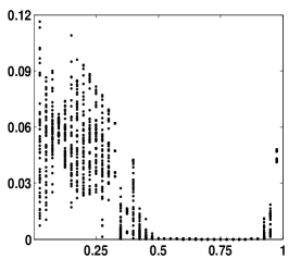
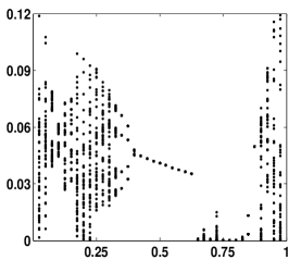
a  b  c 

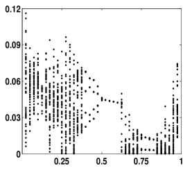
Figure 2: The range of the variance of a typical trajectory of (2.2) on $\operatorname{Cay}({\mathbb{Z}}_{n},B(1))$ as a function of the coupling strength $\epsilon$: a) $n=5$, b) $n=6$, and c) $n=7.$

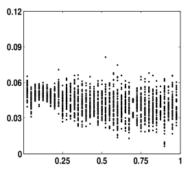
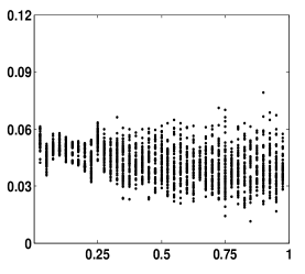
a  b  c 

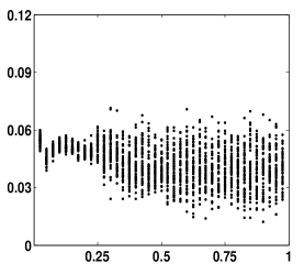
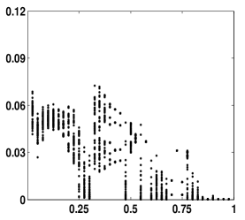
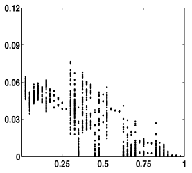
d  e  f 

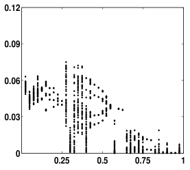
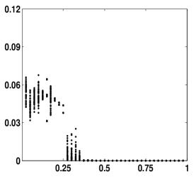
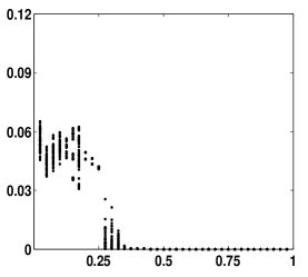
g  h  i 

Figure 3: The range of the variance of a typical trajectory of (2.2) on $\operatorname{Cay}({\mathbb{Z}}_{n},B(r))$ as a function of the coupling strength $\epsilon$: a) $n=100,$ $r=10$, b) $n=200,$ $r=20,$ and c) $n=400,$ $r=40$, d) $n=100,$ $r=25$, e) $n=200,$ $r=50,$ and f) $n=400,$ $r=100$, g) $n=100,$ $r=49$, h) $n=200,$ $r=98,$ and i) $n=400,$ $r=196$.

We now turn to $\Gamma=\operatorname{Cay}({\mathbb{Z}}_{n},B(r))$ for $r\in{\mathbb{N}}$ and $n>2r$. This is the case of the $r$-nearest-neighbor coupling.

Example 3.6.

For $\Gamma=\operatorname{Cay}({\mathbb{Z}}_{n},B(r))$, using (3.3), we have

$$\lambda_{x} = 1-{1\over 2r}\left(\sum_{k=-r}^{r}\cos\left({2\pi xk\over n}\right)-1\right)$$ (3.12)

$$= 1-{1\over 2r}\left({\sin\left({\pi x(2r+1)\over n}\right)\over\sin\left({\pi x\over n}\right)}-1\right),\;x\in[n-1].$$

Using the Taylor’s formula, after straightforward calculations from (3.12) we estimate

$$0<\lambda_{min}\leq\lambda_{1}={\pi^{2}(2r+1)(r+1)\over 3n^{2}}+O(n^{-4}).$$ (3.13)

To estimate $\lambda_{max}$ we use $x^{*}=\lfloor{n\over 2r+1}\rfloor$. For fixed $r\geq 1$ and $n\gg 1$, using Taylor’s formula and elementary inequalities, we estimate

$$\sin\left({\pi\over 2r+1}\right) \leq \sin\left({\pi x^{*}\over n}\right)\leq\sin\left({\pi\over 2r+1}\right)+O(n^{-1}),$$

$${-\pi(2r+1)\over n}+O(n^{-2}) \leq \sin\left({\pi(2r+1)x^{*}\over n}\right)\leq\sin\left({\pi\over 2r+1}\right)+O(n^{-1}).$$

Thus,

$$\lambda_{max}\geq\lambda_{x^{*}}\geq 1+(2r)^{-1}+O(n^{-1})$$

and

$${\lambda_{max}\over\lambda_{min}}\geq{3n^{2}\over\pi^{2}2r(r+1)}+O(n^{-1}).$$ (3.14)

Estimate (3.14) shows that for any fixed $r\in{\mathbb{N}}$ the coupled system (2.2) may satisfy (2.13) for small $n$ and fails to do so starting with some critical network size $n^{*}(r)$ (see Fig. 3 a-c). For larger values of $r$, (2.2) satisfies (2.13) for larger $n$. In this respect, the present case is not different from the nearest-neighbor coupled networks, which we discussed in Example 3.5. The situation changes if we consider nonlocal coupling, i.e., $r=\lfloor\rho n\rfloor$ with the range of coupling $\rho\in(0,0.5)$. Then clearly for not too small $\rho$, one can have (2.13) even for $n\gg 1$.

3.2 The complete, random, and quasirandom graphs

The complete graph on $n$ nodes $K_{n}=(V,E)$ is defined by $V=[n]$ and $E=\{ij:1\leq i<j\leq n\}$.

Lemma 3.7.

The normalized graph Laplacian of $K_{n}$ has a simple zero EV and the EV $1+(n-1)^{-1}$ of multiplicity $n-1$.

Proof. Since $K_{n}$ is a connected $(n-1)$-regular graph, the zero EV of $L(K_{n})$ is simple, and $\mathbf{1}_{n}$ is the corresponding eigenvector (cf. (2.7)). Next, note that any nonzero vector $v=(v_{1},v_{2},\dots,v_{n})$ orthogonal to $\mathbf{1}_{n}$ is an eigenvector of $L(K_{n})$. Indeed, suppose $v_{i}\neq 0$ for some $i\in[n]$. Then

$$(L(K_{n})v)_{i}=v_{i}-{1\over n-1}\sum_{j=2}^{n}v_{j}=\left(1+{1\over n-1}\right)v_{i},$$

where the orthogonality condition $\sum_{j=1}^{n}v_{j}=0$ was used.
$\square$

Therefore, the synchronization condition (2.13) always holds for $\Gamma=K_{n},$ $n\geq 2$. Furthermore, for sufficiently large $n$, the synchronization interval (2.14) is nonempty, and is practically independent of $n$. The windows of synchronization shown in Fig. 4 a-c do not change as the size of the graph increases from $n=10$ in Fig. 4a to $n=100$ in Fig. 4c. Below we consider (2.2) on several graphs that approximate $K_{n}$ and, like $K_{n}$, exhibit good synchronization properties.

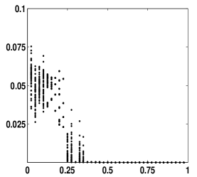
a  b  c 

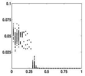
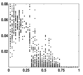
d  e  f 

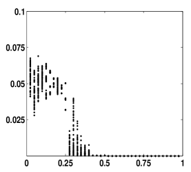
g  h  i 

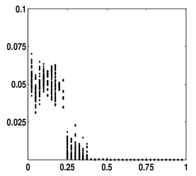
Figure 4: The range of the variance of typical trajectories of (2.2) on $K_{n}$ (a-c), $G(n,1/2)$ (d-f), and Paley (g-i) graphs plotted versus the coupling strength parameter $\epsilon$. The graph sizes are a) $n=10,$ b) $n=50,$ c) $n=100,$ d) $n=10,$ e) $n=50,$ f) $n=100$, g) $n=13,$ h) $n=53,$ and i) $n=101$.

We begin with the classical Erdős-Rényi (ER) model of random graphs [6]. In this model, the edge between every pair $ij,1\leq i<j\leq n,$ is inserted with probability $p$. The decision for a given pair is made independently from the decisions on other pairs. The resultant graph on $n$ nodes is denoted by $G(n,p)$ (see Fig. 1c). The nonzero EVs of $G(n,p)$ satisfy

$$\max_{i\geq 2}|1-\lambda_{i}|\leq O(n^{-1/2})$$ (3.15)

almost surely (cf. [9, 31]). Therefore, from the synchronization viewpoint ER random graphs are as good as complete graphs. They also have considerably fewer edges than $K_{n}$, because the expected degree of edges in $G(n,p)$ is $pn(n-1)/2$.

The EV concentration results in [9] apply to some other random graph models including power-law graphs (see also [10]). Specifically, let $G(w)$ be a random graph on $n$ nodes with a specified expected degree sequence $w=(w_{1},w_{2},\dots,w_{n})$ [8]. Chung-Lu random graphs on a vertex set $V=[n]$ can be constructed by inserting an edge between $i$ and $j$ from $V$ with probability $p_{ij}=w_{i}w_{j}\left(\sum_{k=1}^{n}w_{k}\right)^{-1}$. Here, we assume $\max_{i\in V}w_{i}^{2}\leq\sum_{k=1}^{n}w_{k}$ and allow for loops. Further, for a given power law exponent $\beta$, maximum degree $m$, and average degree $d$, one can generate a power-law graph by setting (cf. [10])

$$w_{i}=c(i+i_{0})^{-1/\beta-1},\;1\leq i\leq n,$$

where

$$c={\beta-2\over\beta-1}dn^{1/\beta-1}\quad\mbox{and}\quad i_{0}=\left({d(\beta-2)\over m(\beta-1)}\right)^{\beta-1}.$$

For Chung-Lu power-law graphs, Theorem 9 in [10] then guarantees that all positive EVs are localized

$$\left|\lambda_{k}(L)-1\right|=o(1),\;k\geq 2,$$

with probability $1-o(1)$ provided $\min_{i\in V}w_{i}\gg\operatorname{ln}n$. In Fig. 5 we present numerical results for the coupled system (2.2) on Chung-Lu power-law graphs for two values of the expected degree, $d$. For both values of $d$, Fig. 5 shows large windows of synchronization.

a  b 

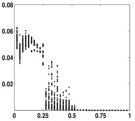
Figure 5: The range of the variance of typical trajectories of (2.2) on the power-law graphs on $200$ nodes. The degree distribution of the graphs used in all three plots is $\sim k^{-3}$. The average degree is a) $d=20$ and b) $d=30$.

Next, we turn to quasirandom graphs, which share many combinatorial properties with the ER graphs $G(n,p)$ (cf. [7, 19]). Below, we restrict to the case $p=1/2$ and consider only $d$-regular graphs. There are several equivalent properties that define a quasirandom graph $\Gamma=(E,V)$ [7]. For instance, for any $S\subset V,\;(|V|=n)$, the number of edges connecting the nodes in $S$ is

$${1\over 4}|S|^{2}+O(n^{2}),$$ (3.16)

exactly as for the ER graph $G(n,1/2)$. If $\Gamma$ is a $d$-regular graph then (3.16) is equivalent to the following localization property of the nonzero EVs of the normailized graph Laplacian (cf. Theorem 9.3.1, [3])

$$\left|\lambda_{i}-1\right|=o(1),\;i=2,3,\dots,n.$$ (3.17)

Hence, for coupled systems on quasirandom graphs synchronization condition (2.13) holds for sufficiently large $n$ and, as in the case of the complete graph, the interval of synchronization (2.14) to leading order is independent of $n$ for $n\gg 1$ (see Fig. 4 d-f). To illustrate synchronization properties of (2.2) on quasirandom graphs, we use Paley graphs, which are defined as follows.

Example 3.8.

Let $n=1\pmod{4}$ be a prime and denote

$${\mathbb{Z}}^{\times}_{n}={\mathbb{Z}}_{n}/\{0\}\quad\mbox{and}\quad Q_{n}=\{x^{2}\pmod{n}:\;x\in{\mathbb{Z}}_{n}^{\times}\}.$$

$Q_{n}$ is viewed as a set (not multiset, i.e., each element has multiplicity $1$). Then $Q_{n}$ is a symmetric subset of $Z_{n}^{\times}$ and $|Q_{n}|=2^{-1}(n-1)$ (cf. [18, Lemma 7.22]). $P_{n}=\operatorname{Cay}(Z_{n},Q_{n})$ is called a Paley graph [18].

The nonzero EVs of $L(P_{n})$ can be computed explicitly from (3.3), using properties of the Gauss sum (cf. [18]):

$$\lambda_{x}(P_{n})=\left\{\begin{array}[]{ll}1+{1-\sqrt{n}\over n-1},&x\mbox{ is a QR}~{}\pmod{n},\\ 1+{1+\sqrt{n}\over n-1},&x\mbox{ is not a QR}~{}\pmod{n},\end{array}\right.$$ (3.18)

where $x\in{\mathbb{Z}}_{n}^{\times}$.

The numerical results for the coupled system (2.2) on Paley graphs show good agreement with the analytical estimates. The synchronization windows computed numerically for (2.2) on Paley graphs are as large as those for the complete graphs of the same size (see Fig. 4 g-i). Overall, the variance plots for (2.2) on the complete, ER, and Paley graphs in Fig. 4 have a great degree of similarity.

3.3 Expanders

The complete, random, and quasirandom graphs endow the coupled system (2.2) with good synchronization properties but at a price of having $O(n^{2})$ edges in a graph of size $n$. In this subsection, we will review certain families of graphs with much fewer edges, which nonetheless approximate complete graphs and promote synchronization in coupled systems like (2.2).

Let $\Gamma_{n}=(V(\Gamma_{n}),E(\Gamma_{n})),n\in{\mathbb{N}},$ be a family of $d$-regular connected graphs. Suppose $V(\Gamma_{n})=[n]$ and denote the EVs of $L(\Gamma_{n})$ by

$$0=\lambda_{1}<\lambda_{2}\leq\dots\leq\lambda_{n}.$$

By Gershgorin’s Theorem [14], $\lambda_{n}\leq 2d$. Therefore, the most likely way for the synchronization condition (2.13) to break down for large $n$ is through the second EV $\lambda_{2}(\Gamma_{n})$ approaching $0$. This leads us to consider families of graphs, for which the second EV remains bounded away from zero

$$\lambda_{2}(\Gamma_{n})\geq c_{1}>0.$$ (3.19)

Such families of graphs are called expanders [35].

Definition 3.9.

[34, 18] A family of $d$-regular graphs $\Gamma_{n}=(V(\Gamma_{n}),E(\Gamma_{n})$ ($|V(\Gamma_{n})|\to\infty$ as $n\to\infty$) is called an expander family if the Cheeger constant

$$h(\Gamma_{n})=\min_{F}{|\partial F|\over\min\{|F|,|V(\Gamma_{n})/F|\}}\geq c_{2}>0\;\forall n,$$ (3.20)

where the minimum is taken over all proper subsets of $V(\Gamma_{n})$, $F\neq\emptyset$, and $\partial F$ stands for the set of edges connecting the nodes in $F$ with the nodes in the complement of $F$, $V(\Gamma_{n})/F$.

The Cheeger constant $h(\Gamma)$ quantifies the connectivity of $\Gamma$. The uniform bound on $h(\Gamma_{n})$ in (3.20) guarantees that $\Gamma_{n}$ remain well-connected even as $|V(\Gamma_{n})|$ grows without a bound. The combinatorial condition (3.20) is equivalent to the spectral one (3.19) (cf. [2, 1]), which we arrived at in the context of synchronization. Therefore, synchronizability in large networks is directly related to connectivity: the better connected large networks are, the more likely they to satisfy the synchronization condition (2.13). The connectivity is better in graphs with larger second EV $\lambda_{2}$ [11]. There is an upper bound on $\lambda_{2}(\Gamma_{n})$ (cf. [13]):

$$\limsup_{n\to\infty}\lambda_{2}(\Gamma_{n})\leq d-2\sqrt{d-1}.$$ (3.21)

A family of graphs $\{\Gamma_{n}\}$ is called Ramanujan if

$$\lambda_{2}(\Gamma_{n})\geq d-2\sqrt{d-1}.$$

Ramanujan graphs exhibit the optimal asymptotics of $\lambda_{2}(\Gamma_{n})$ and, in this sense, possess the best possible connectivity. By inspecting several common families of $d$-regular graphs, such as the nearest-neighbor graphs, one can see that typically the second EV tends to $0$ rapidly as $n\to\infty$ (see, e.g., (3.13)). In fact, any family of Cayley graphs of bounded degree on an abelian group can not be an expander family [18, §4.3]. Nontheless, a typical family of random $d$-regular graphs ($d\geq 3$) is very close to be Ramanujan with high probability as shown in [12]. The deterministic constructions of expander families are also available, albeit they rely on sophisticated algebraic techniques (cf., [22, 21, 34]).

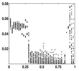
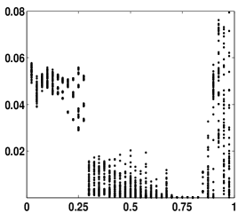
a  b  c 

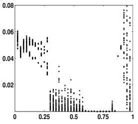
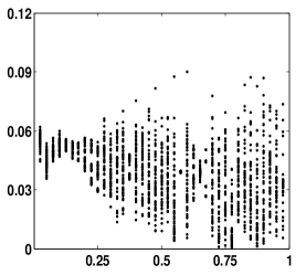
d  e  f 

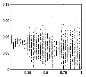
Figure 6: The range of the variance of typical trajectories of (2.2) on the random bipartite graphs (cf. Example 3.10). The graphs used in these simulations have $400$ nodes. The degrees are a) $10,$ b) $15,$ and c) $20.$ For comparison, in plots d-f, we included numerical results for the coupled system on Cayley graphs with regular connections $\operatorname{Cay}(Z_{n},B(r))$ for d) $n=100,r=10$, e) $n=200,r=20$, and f) $n=400,r=40$.

To illustrate synchronization in coupled systems on expanders, we will use the following family of random bipartite $d$-regular graphs.

Example 3.10.

Let $B_{2m,d},m\geq 2$ be a bipartite graph on $2m$ vertices. The edges are generated using the following algorithm:

1. Let $p:[m]\to[m]$ be a random permutation. In our numerical experiments, we used MATLAB function $\mathsf{randperm}$ to generate random permutations. For $i\in[m]$, add edge $(i,m+p(i))$.

2. Repeat step 1. $d-1$ times.

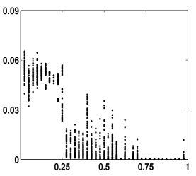
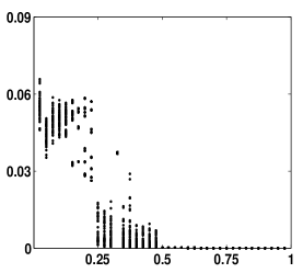
a  b  c 

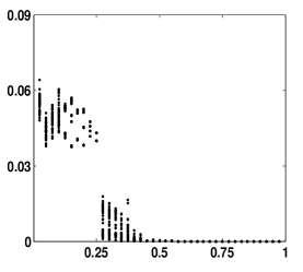
Figure 7: The range of the variance of typical trajectories of (2.2) on the random Cayley graph $\operatorname{Cay}({\mathbb{Z}}_{n},\pm R_{k})$: a) $n=100$, $k=10$, b) $n=200$, $k=20$, and c) $n=400$, $k=40$.

The numerical results in Fig. 6 show that coupled system on $B_{400,15}$ already has a notable window of synchronization (see Fig. 6b), which becomes even bigger for $B_{400,20}$ (see Fig. 6c). Note that in the present case we do not have localization results for the EVs of $L$, as in the analysis of the coupled system (2.2) on random and quasirandom graphs (cf. (3.15), (3.17)), and we can only rely on the lower bound for $\lambda_{2}$ (3.19). Therefore, for chaotic dynamical systems on expanders, in general, we can not guarantee that synchronization condition (2.13) holds for all $n\gg 1$. Nonetheless, as can be seen from the numerical results in Fig. 6 a-c, one can achieve synchronization on large expanders of relatively small degree. The numerical results for the bipartite random graphs may be compared to the results for the Cayley graphs on $B(r)$ in Fig. 6 d-f, which show that the coupled system (2.2) on smaller graphs of the same degree but with regular connections remains rather far from synchrony. This is another illustration of the advantages of random connectivity for synchronization.

In conclusion, we consider synchronization of the coupled system (2.2) on random Cayley graphs
$\operatorname{Cay}({\mathbb{Z}}_{n},\pm R_{k})$, where $R_{k}$ is a set of $k$ elements chosen from the uniform distribution on ${\mathbb{Z}}_{\lfloor n/2\rfloor}$. Random Cayley graphs are expanders with high probability for $n\gg 1$ and $k=O(\log n)$ [20]. The numerical results for the dynamical systems on random Cayley graphs in Fig. 7 show that these systems exhibit much better synchronization properties than the systems on regular Cayley graphs of the same size (see Fig. 6 d-f).

4 Discussion

Motivated by the linear stability analysis in [16], in this paper, we rigorously derived a sufficient condition for synchronization in systems of diffusively coupled maps, whose dynamics can be chaotic. In contrast to the approach in [16], we did not seek to show asymptotic stability of spatially homogeneous solutions of (2.2)

$$\mathbf{x}_{k}=x_{k}\mathbf{1}_{n},\;k=0,1,2,\dots,$$ (4.1)

where $\{x_{k}\}$ is a trajectory of the local system (2.1). Instead, we proved the asymptotic stability of the invariant subspace of such solutions $\mathcal{D}$ (cf. (2.7)), in the sense that every trajectory of (2.2) that started sufficiently close from $\mathcal{D}$ approaches $\mathcal{D}$ in forward time. Note that the asymptotic stability of $\mathcal{D}$ does not imply the asymptotic stability of individual trajectories (4.1). In particular, our approach circumvents the analysis of perturbations in the tangential to $\mathcal{D}$ direction, which would be necessary for the justification of the linearization about (4.1). The latter problem is quite technical already in the case when local systems have stable dynamics [23]. On the other hand, it is not clear that for coupled chaotic systems one has sufficient control over perturbations in the tangential direction, because it corresponds to a degenerate subspace of the coupling matrix and the local dynamics are sensitive to perturbations.

The sufficient condition for synchronization (2.13) identifies the complete graph as an optimal network organization for chaotic synchronization. Therefore, in the second part of this paper, we considered networks on graphs that approximate the complete graph. These include ER random graphs, as well as quasirandom and Chung-Lu power-law graphs. We show that from synchronization point of view these graphs are almost as good as the complete graph provided that the network is large enough. Furthermore, expanders, which constitute a broader class of graphs, tend to have good synchronization properties. As many of these graphs are constructed using random algorithms, our results highlight the advantages of random connectivity for synchronization.

Acknowledgements. This work was supported in part by the NSF grants DMS 1109367 and DMS 1412066 (to GSM).

References

- [1] N. Alon, Eigenvalues and expanders, Combinatorica 6 (1986), no. 2, 83–96.
- [2] N. Alon and V. D. Milman, isoperimetric inequalities for graphs, and superconcentrators, J. Combin. Theory Ser. B 38 (1985), no. 1, 73–88. MR 782626 (87b:05092)
- [3] Noga Alon and Joel H. Spencer, The probabilistic method, third ed., Wiley-Interscience Series in Discrete Mathematics and Optimization, John Wiley & Sons Inc., Hoboken, NJ, 2008, With an appendix on the life and work of Paul Erdős. MR 2437651 (2009j:60004)
- [4] Albert-László Barabási and Réka Albert, Emergence of scaling in random networks, Science 286 (1999), no. 5439, 509–512. MR 2091634
- [5] N. Biggs, Algebraic Graph Theory, second edition ed., Cambridge University Press, 1993.
- [6] Béla Bollobás, Modern graph theory, Graduate Texts in Mathematics, vol. 184, Springer-Verlag, New York, 1998. MR 1633290 (99h:05001)
- [7] F. R. K. Chung, R. L. Graham, and R. M. Wilson, Quasirandom graphs, Proc. Nat. Acad. Sci. U.S.A. 85 (1988), no. 4, 969–970. MR 928566 (89a:05116)
- [8] Fan Chung and Linyuan Lu, Connected components in random graphs with given expected degree sequences, Ann. Comb. 6 (2002), no. 2, 125–145. MR 1955514 (2003k:05123)
- [9] Fan Chung, Linyuan Lu, and Van Vu, Spectra of random graphs with given expected degrees, Proc. Natl. Acad. Sci. USA 100 (2003), no. 11, 6313–6318. MR 1982145 (2004e:05175)
- [10] Fan Chung and Mary Radcliffe, On the spectra of general random graphs, Electron. J. Combin. 18 (2011), no. 1, Paper 215, 14. MR 2853072 (2012j:05358)
- [11] M. Fiedler, Algebraic connectivity of graphs, Czech. Math. J. 23(98) (1973).
- [12] Joel Friedman, A proof of Alon’s second eigenvalue conjecture and related problems, Mem. Amer. Math. Soc. 195 (2008), no. 910, viii+100. MR 2437174 (2010e:05181)
- [13] S. Hoory, N. Linial, and A. Wigderson, Expander graphs and their applications, Bull. Amer. Math. Soc. (N.S.) 43 (2006), no. 4, 439–561 (electronic). MR 2247919 (2007h:68055)
- [14] Roger A. Horn and Charles R. Johnson, Matrix analysis, second ed., Cambridge University Press, Cambridge, 2013. MR 2978290
- [15] P. Jiruska, M. de Curtis, J.G. Jefferys, Schevon C.A., Schiff S.J., and K. Schindler, Synchronization and desynchronization in epilepsy: controversies and hypotheses, J. Physiol. 591 (2013), 787–97.
- [16] J. Jost and M. P. Joy, Spectral properties and synchronization in coupled map lattices, Phys. Rev. E 65 (2001), 016201.
- [17] Hüseyin Koçak and Kenneth J. Palmer, Lyapunov exponents and sensitivity dependence, J. Dynam. Differential Equations 22 (2010), no. 3, 381–398. MR 2719912 (2012f:37075)
- [18] M. Krebs and A. Shaheen, Expander Families and Caley Graphs: A Beginner’s Guide, Oxford University Press, 2011.
- [19] M. Krivelevich and B. Sudakov, Pseudo-random graphs, More sets, graphs and numbers, Bolyai Soc. Math. Stud., vol. 15, Springer, Berlin, 2006, pp. 199–262. MR 2223394 (2007a:05130)
- [20] Zeph Landau and Alexander Russell, Random Cayley graphs are expanders: a simple proof of the Alon-Roichman theorem, Electron. J. Combin. 11 (2004), no. 1, Research Paper 62, 6. MR 2097328 (2005g:05069)
- [21] A. Lubotzky, R. Phillips, and P. Sarnak, Ramanujan graphs, Combinatorica 8 (1988), no. 3, 261–277. MR 963118 (89m:05099)
- [22] G. A. Margulis, Explicit group-theoretic constructions of combinatorial schemes and their applications in the construction of expanders and concentrators, Problemy Peredachi Informatsii 24 (1988), no. 1, 51–60. MR 939574 (89f:68054)
- [23] G.S. Medvedev, Synchronization of coupled limit cycles, J. Nonlinear Sci. 21 (2011), no. 3, 441–464. MR 2823863 (2012g:34092)
- [24] , Stochastic stability of continuous time consensus protocols, SIAM Journal on Control and Optimization 50 (2012), no. 4, 1859–1885.
- [25] G.S. Medvedev and S. Zhuravytska, The geometry of spontaneous spiking in neuronal networks, Journal of Nonlinear Science 22 (2012), 689–725.
- [26] , Shaping bursting by electrical coupling and noise, Biological Cybernetics 106 (2012), 67–88, 10.1007/s00422-012-0481-y.
- [27] Adilson E. Motter, Seth A. Myers, Marian Anghel, and Takashi Nishikawa, Spontaneous synchrony in power-grid networks, Nat. Phys. 9 (2013), no. 3, 191–197.
- [28] Takashi Nishikawa and Adilson E. Motter, Network synchronization landscape reveals compensatory structures, quantization, and the positive effect of negative interactions, Proceedings of the National Academy of Sciences 107 (2010), no. 23, 10342–10347.
- [29] Reza Olfati-Saber, J Alex Fax, and Richard M Murray, Consensus and cooperation in networked multi-agent systems, Proceedings of the IEEE 95 (2007), no. 1, 215–233.
- [30] Reza Olfati-Saber and Richard M Murray, Consensus problems in networks of agents with switching topology and time-delays, Automatic Control, IEEE Transactions on 49 (2004), no. 9, 1520–1533.
- [31] R.I. Oliveira, Concentration of the adjacency matrix and of the laplacian in random graphs with independent edges, arXiv:0911.0600 (2010).
- [32] Louis M. Pecora and Thomas L. Carroll, Synchronization in chaotic systems, Phys. Rev. Lett. 64 (1990), no. 8, 821–824. MR 1038263 (92c:58082)
- [33] Arkady Pikovsky, Michael Rosenblum, and Jürgen Kurths, Synchronization, Cambridge Nonlinear Science Series, vol. 12, Cambridge University Press, Cambridge, 2001, A universal concept in nonlinear sciences. MR 1869044 (2002m:37001)
- [34] Omer Reingold, Salil Vadhan, and Avi Wigderson, Entropy waves, the zig-zag graph product, and new constant-degree expanders, Ann. of Math. (2) 155 (2002), no. 1, 157–187. MR 1888797 (2003c:05145)
- [35] Peter Sarnak, What isan expander?, Notices Amer. Math. Soc. 51 (2004), no. 7, 762–763. MR 2072849
- [36] Steven Strogatz, Sync, Hyperion Books, New York, 2003, How order emerges from chaos in the universe, nature, and daily life. MR 2394754
- [37] G.F. Young, L. Scardovi, and N.E. Leonard, Robustness of noisy consensus dynamics with directed communication, Proceedings of the American Control Conference, Baltimore, MD (2010).