Highly corrupted image inpainting through hypoelliptic diffusion

Abstract

We present a new bio-mimetic image inpainting algorithm, the Averaging and Hypoelliptic Evolution (AHE) algorithm, inspired by the one presented in (U. Boscain et al. SIAM J. Imaging Sci., 7(2):669–695, 2014) and based upon a semi-discrete variation of the Citti–Petitot–Sarti model of the primary visual cortex V1. The AHE algorithm is based on a suitable combination of sub-Riemannian hypoelliptic diffusion and ad-hoc local averaging techniques. In particular, we focus on highly corrupted images (i.e., where more than the 80% of the image is missing), for which we obtain high-quality reconstructions.

1 Introduction

In art, image inpainting refers to the practice of (manually) retouching damaged paintings in order to remove cracks or to fill-in missing patches. Within the past decade the digital version of image inpainting, i.e., the reconstruction of digital images by means of different types of automatic algorithms, has received increasing attention.

In this paper, we present a new bio-mimetic inpainting algorithm (called AHE), which is applicable to highly corrupted images with a general corruption. Several examples of reconstructions obtained with the AHE algorithm are presented in Fig. 6 – 8 at the end of the paper.

The starting point of our work is the Citti–Petitot–Sarti model of the primary visual cortex V1 Petitot2008 ; Petitot2003 ; Citti2006 ; Sanguinetti , and our recent contributions Remizov2013 ; Boscain2010 ; Boscain2012a ; Boscain2014 ; Duits2014 ; PrandiBohi . This model has also been deeply studied in Duits2008 ; Duits2010 ; Duits2010a ; Hladky2010 . The main idea behind the Citti–Petitot–Sarti model is the geometric model of vision called pinwheel model, going back to the 1959 paper HUBEL1959a . Here, Hübel and Wiesel showed that cells in the mammals primary visual cortex V1 do not only deal with positions in the visual field, but also with orientation information: actually there are groups of neurons that are sensitive to position and directions with connections between them that are activated by the image. The system of connections between neurons, called the functional architecture of V1, preferentially connects neurons detecting alignements. This is the so-called pinwheels structure of V1. In the Citti–Petitot–Sarti model, V1 is then modeled as a 3D manifold endowed with a sub-Riemannian structure that mimics these connections as a continuous limit. The natural way to inpaint the missing regions of an image is thus by using the hypoelliptic diffusion associated with this structure.

In Remizov2013 we proposed a semi-discrete version of the Citti–Petitot–Sarti model that considers a continuous structure in the space of positions, but a discrete structure for the orientation information, which makes sense from the neuro-physiological point of view Petitot2008 . Image reconstruction methods based upon this principle are presented in detail in the previous works Remizov2013 ; Boscain2012a . The same techniques are applied to the semi-discrete hypoelliptic evolution associated with the well-known Mumford elastica model in visionCDC and to image recognition in PBG2015 ; PrandiBohi . See gros-papier for a survey of these methods.

In the above mentioned works, the main focus was on inpainting algorithms where no prior knowledge on the location of the corruption was needed. However, in Remizov2013 we presented a way to exploit this knowledge by introducing certain heuristic procedures that, together with the hypoelliptic diffusion, yield drastically better inpainting results. In this paper, we improve on this result, and thus we will henceforth assume complete knowledge of the location and shape of the corrupted areas of the image.

Our study is focused on improving the local methods developed in Remizov2013 . Indeed, we manage to obtain state-of-the-art results for highly corrupted images where no “big” regions are missing, i.e., where non-corrupted pixels are “well distributed”. See the conclusions and Fig. 10, for more details on this fact.

Namely, we improve on the semi-discrete approach proposed in Remizov2013 for the Citti–Petitot–Sarti model, by introducing heuristic methods that allow us to treat images with more than 80% (and even more than 90%) of corrupted pixels, see Fig. 7 – 8 in the end of the paper. In particular, the reconstructions of Fig. 6 are comparable with those obtained in Masnou2002 for images with 65% of corrupted pixels, but no assumption of simple connectedness on the corrupted part is needed.

For some types of corrupted images, our results are comparable with those of Citti2016 . They use a different approach, combining the sub-Riemannian model with a diffusion/concentration process, which in the limit corresponds to a mean curvature flow. It is interesting to notice that the two approaches provides slightly different results depending on the quantity of corruption. However, highly corrupted images are not considered in Citti2016 .

It is well-known that when treating large corruptions and fine textures, the best results are often obtained via copy-and-paste texture synthesis Bugeau2010 . Although it would be interesting to combine these methods with the bio-mimetic approach presented here, this is outside the scope of the current work.

The paper is organized as follows.

• In Section 2 we briefly recall the basic principles of the method introduced in Remizov2013 ; Boscain2012a and discuss some of its properties. Moreover, we present some numerical experiments showing the anisotropicity of the diffusion. (See Fig. 1 – 3). We also recall the SR/DR procedure, presented in Remizov2013 , that allows for better reconstructions by exploiting the informations on the location of the corruption.

• In Section 3 we present a first improvement of this method, where an hypoelliptic diffusion with varying coefficients is considered. The coefficients are chosen for the effect of the anisotropic diffusion to be faster where the corruption is present. When coupled with the DR procedure, this algorithm gives good results if the corrupted parts are narrow, e.g., in the case of vertical and horizontal lines as in Fig. 4. However, it does not provide good quality inpaintings of highly corrupted images as is evident from Fig. 9. This motivates the further development of this method, which is presented in the next section.

• Section 4 contains the main result of this paper: the Averaging and Hypoelliptic Evolution (AHE) algorithm. This method is a synthesis of two different approaches to image reconstruction: the hypoelliptic diffusion with varying coefficients and a suitable averaging procedure. As shown in Fig. 6 – 8, this method allows for good reconstructions of highly corrupted images. In Section 4.5, we also present a simple analysis of the complexity of the AHE algorithm as a function of the image size.

• Finally, in Fig. 9 we present a comparison of reconstructions obtained via the methods presented in this paper.

Let us remark that, although all the numerical experiments of this paper are obtained on $256\times 256$ pixels images, the proposed methods are resolution-agnostic. The techniques presented are targeted to greyscale images, but no difficulty arises in applying them to the separate channels of color images. Different adaptations of these techniques to color images are possible, but not investigated here.

Finally, we stress that it is outside the scope of this paper to present comparisons with other algorithms or to provide a complete list of references on this problem. We point the interested reader to Bugeau2010 ; Bertalmio2000 ; Chan2002 ; Citti2016 ; Facciolo ; Masnou1998 ; Wang2013 and references therein. It is worth observing that it is difficult to measure objectively the quality of a reconstruction, see, for instance, voronin ; zhang ; Ponomarenko . Moreover, such a measure will forcibly depend on the expected application.

2 The model and previous results

2.1 Images under consideration

Mathematically, a greyscale image is a function $f\colon\Pi\to[0,1]$, where $\Pi$ is a square on the $(x,y)$-plane. If $f(x,y)=0$ the color of the image at $(x,y)$ is white, while if $f(x,y)=1$ it is black. We will consider $\Pi$ as a periodic subgroup of ${\mathbb{R}}^{2}$ endowed with its Haar measure. Since the corresponding Haar measure is finite, all images are square integrable by definition. This also allows to consider images as $\Pi$-periodic functions $f:{\mathbb{R}}^{2}\to[0,1]$.

Together with the above continuous model we consider also the corresponding discrete model: A greyscale image $f$ is stored as an $(M\times M)$-matrix, where for simplicity we are assuming the same number of pixels vertically and horizontally. As before we assume $f_{kl}\in[0,1]$, $k,l\in\{1,\ldots,M\}$. Then, given a rectangular grid $(x_{k},y_{l})$, $k,l\in\{1,\ldots,M\}$ in the $(x,y)$-plane, the discrete version of an image is the function $(x_{k},y_{l})\mapsto f(x_{k},y_{l}):=f_{kl}$. As before, it is convenient to consider the grid and the functions to be periodic on ${\mathbb{Z}}^{2}$.

Observe that we can assume that $f(x_{k},y_{l})>0$ at any point $(x_{k},y_{l})$ that corresponds to a non-corrupted pixel. Thus, due to the the knowledge of the corrupted part, we can assume that $f(x_{k},y_{l})=0$ if $(x_{k},y_{l})$ corresponds to a corrupted pixel.

2.2 Two models for the diffusion

2.2.1 Hypoelliptic diffusion in the continuous limit model

The main idea of the (continuous) model of the diffusion is then that V1 lifts images, which are $\Pi$-periodic functions $f:{\mathbb{R}}^{2}\to[0,1]$, to functions over the projective tangent bundle $PT\mathbb{R}^{2}$. This bundle has as base $\mathbb{R}^{2}$ and the projective line $P\mathbb{R}$ as fiber at $(x,y)$. Recall that $P\mathbb{R}$ is the set of directions of straight lines lying on the plane and passing through $(x,y)$. This can be represented by the angles $\theta\in[0,\pi]/\sim$, where $\sim$ is the equivalence relation identifying $0$ with $\pi$. In this model, a corrupted image is reconstructed by minimizing the energy necessary to activate the regions of the visual cortex not excited by the image.

Mathematically speaking, the original image $f(x,y)$ is first smoothed through an isotropic Gaussian filter (it is widely accepted that this corresponds to an action at the retinal level, see Marr1980 ; Peichl1979 ). As shown in Boscain2012a this yields a smooth function which is generically of Morse type, i.e., it has isolated non-degenerate critical points only. The smoothed image (that we will still call $f(x,y)$) is then lifted to the (generalized) function $\bar{f}(x,y,\theta)$ on $PT{\mathbb{R}}^{2}$ defined by

$$\overline{f}(x,y,\theta):=f(x,y)\,\delta(g(x,y,\theta)),\quad\text{for}$$ (1)

$$g(x,y,\theta):=\cos\theta\frac{\partial f}{\partial x}(x,y)+\sin\theta\frac{\partial f}{\partial y}(x,y),$$ (2)

where $\delta(\cdot)$ is the Dirac delta function. Moreover, the space $PT{\mathbb{R}}^{2}$, with coordinates $(x,y,\theta)$, is endowed with the sub-Riemannian structure with orthonormal frame $\{X_{1},\sqrt{\beta}X_{2}\}$, where

$$X_{1}(x,y,\theta)=\cos\theta\frac{\partial}{\partial x}+\sin\theta\frac{\partial}{\partial y},$$ (3)

$$X_{2}(x,y,\theta)=\frac{\partial}{\partial\theta}.$$

Here, $\beta$ is a positive parameter, which is a neurophysiological dimensional constant. We refer to Appendix A for a brief introduction to sub-Riemannian geometry.

Notice that the above structure is invariant under the action of the group $SE(2)$ of rototranslations of the plane. Via stochastic considerations (see Remizov2013 ), one is then able to translate the energy minimizing principle expressed above to the fact that the image is evolved according to the hypoelliptic diffusion associated with the above vector fields. (See Section A.1.) Namely, the reconstructed function on $PT{\mathbb{R}}^{2}$ is the solution $\psi=\psi(x,y,\theta,t)$ at time $t=T$ of the initial value problem

$$\left\{\begin{aligned} &\frac{\partial\psi}{\partial t}=\Delta_{H}\psi,\ \ \,\Delta_{H}=(X_{1})^{2}+\beta(X_{2})^{2},\\ &\psi\bigl{|}_{t=0}=\overline{f}(x,y,\theta).\\ \end{aligned}\right.$$ (4)

For image reconstruction purposes, we choose the value of $\beta$ experimentally as well as the the value of the final time $T$.

No boundary condition is needed in diffusion equation (4), since we are considering the diffusion on the whole space $PT{\mathbb{R}}^{2}$ and the initial function $\overline{f}(x,y,\theta)$ is periodic w.r.t. $(x,y,\theta)\in PT{\mathbb{R}}^{2}$. Finally, $\psi$ is projected back to a function on $\mathbb{R}^{2}$, which will be the final result of the image inpainting procedure (see the details in Section 2.3.2). The diffusion equation, up to the tuning of the parameter $\beta$, is the same for all images: The information about the initial image is fed to the evolution only through the initial condition $\overline{f}$.

2.2.2 Semi-discrete alternative to the hypoelliptic diffusion

In Remizov2013 , we proposed a semi-discrete alternative to the Citti–Petitot–Sarti model, by assuming that the number $N$ of directions represented in V1 is finite. It corresponds to the restriction of $SE(2)$, the group of rototranslations of the plane, to rotations with discrete angles

$$\theta_{r}=\frac{2\pi r}{N},\quad r=0,\ldots,N-1.$$

The resulting group is denoted by $SE(2,N)$, and the evaluation of functions $\Psi:SE(2,N)\to\mathbb{R}$ at $(x,y,r)\in SE(2,N)$ by $\Psi^{r}(x,y)$.

Assuming that the probability of jumps between adjacent directions is a Poisson process with parameter $\beta>0$, stochastic considerations similar to those employed in the continuous model lead to the semi-discrete analogue of diffusion equation (4):

$$\left\{\begin{aligned} &\frac{\partial\Psi^{r}(x,y)}{\partial t}=\Delta_{{\cal H}}\Psi^{r}(x,y),\ \ \,\Delta_{{\cal H}}=A+\beta\Lambda_{N},\\ &\Psi^{r}(x,y)\bigl{|}_{t=0}=\overline{f}(x,y,\theta_{r}),\\ \end{aligned}\right.$$ (5)

where $\Delta_{{\cal H}}$ is the semi-discrete analogue of the differential operator $\Delta_{H}$. Namely,

$$A\Psi^{r}(x,y)=\left(\cos{\theta_{r}}\frac{\partial}{\partial x}+\sin{\theta_{r}}\frac{\partial}{\partial y}\right)^{2}\Psi^{r}(x,y),$$

$$\Lambda_{N}\Psi^{r}(x,y)=\Psi^{r-1}(x,y)-2\Psi^{r}(x,y)+\Psi^{r+1}(x,y).$$

This operator is invariant under the action of the semi-discrete rototranslations, given by continuous translations and discrete rotations of angle $\theta_{r}$. Moreover, letting $\beta=(N/2\pi)^{2}$, the semi-discrete operator $\Delta_{\mathcal{H}}$ converges to $\Delta_{H}$ as $N\to+\infty$. (See Remizov2013 .)

2.2.3 Numerical treatement of the hypoelliptic equation

As detailed in Remizov2013 ; visionCDC , there are two possibilities for the numerical integration of equation (5) starting from the lifts of the images described in Section 2.1. We may spatially discretize the equation and then apply the discrete Fourier transform w.r.t. $x,y$ in order to decouple the frequencies, or we may interpolate the initial datum $\bar{f}$ via almost-periodic functions and exploit their properties.

Both strategies lead to similar fully-discrete equations, although the second strategy leads to exact solutions in the class of almost-periodic functions. Since the final results are essentially the same, we detail here only the first type of discretization, which is simpler to present.

We consider the discrete Fourier transforms of the interpolations of the functions $\Psi^{r}$ on the fixed $M\times M$ spatial grid of Section 2.1. This is given by the formula

$$\hat{\Psi}_{k,l}^{r}=\frac{1}{M}\sum_{n,m=1}^{M}\Psi_{n,m}^{r}e^{-2\pi i\left(\frac{(k-1)(n-1)}{M}+\frac{(l-1)(m-1)}{M}\right)}.$$

Exploiting the above, we are led to a completely decoupled system of $M^{2}$ linear evolution equations of Mathieu type over ${\mathbb{C}}^{N}$:

$$\frac{d\hat{\Psi}_{k,l}}{dt}=\bigl{(}\Lambda_{N}-\beta M\text{diag}_{p}(a_{k,l}^{p})^{2}\bigr{)}\hat{\Psi}_{k,l},$$ (6)

where $\hat{\Psi}_{k,l}=(\hat{\Psi}^{1}_{k,l},\ldots,\hat{\Psi}^{N}_{k,l})^{\mathrm{T}}$, and we let

$$(\Lambda_{N}\hat{\Psi}_{k,l}^{r})_{r}=\hat{\Psi}_{k,l}^{r-1}-2\hat{\Psi}_{k,l}^{r}+\hat{\Psi}_{k,l}^{r+1},$$

$$a_{k,l}^{p}=\cos(\theta_{p})\sin\left(2\pi\frac{k-1}{M}\right)+\sin(\theta_{p})\sin\left(2\pi\frac{l-1}{M}\right).$$

We refer to Remizov2013 for details.

Each of the evolution equations (6) can be independently solved via standard numerical semi-implicit schemes, recommended for this type of equation (see (Marchuk1982, , Chapter 5)).

2.3 The reconstruction algorithm

The algorithm for image inpainting via hypoelliptic diffusion is divided in three steps:

1. Lift the image $f(x_{k},y_{l})$ to $\overline{f}(x_{k},y_{l},\theta_{r})$.

2. Evolve $\overline{f}(x_{k},y_{l},\theta_{r})$ according to (6) after passing to the frequency grid: $\bar{f}\mapsto\hat{\bar{f}}$. This step was already discussed in Section 2.2.3.

3. Go back to the spatial grid by inverse discrete Fourier transform and project the result back to the original 2-dimensional grid.

2.3.1 Lift

The discrete analogue of the initial function $\overline{f}$ defined in (1), (2) has the form:

$$\overline{f}(x_{k},y_{l},\theta_{r})=\left\{\begin{aligned} f(x_{k},y_{l}),\ \ \,&\textrm{if}\ \ \theta_{r}\simeq\theta(k,l),\\ \phantom{0}0,\phantom{000}\ \ \,&\textrm{if}\ \ \theta_{r}\not\simeq\theta(k,l).\\ \end{aligned}\right.$$ (7)

Here, $\theta(k,l)$ is the discrete analogue of the slope angle of the level curve $\{f(x,y)={\text{const}}\}$ passing through the point $(x_{k},y_{l})$, that is,

$$\tan\theta(k,l)=-\frac{f_{x}}{f_{y}}(x_{k},y_{l}),$$ (8)

where $f_{x}$ and $f_{y}$ are the standard finite-difference analogues of the corresponding partial derivatives. The notation $\theta_{r}\simeq\theta(k,l)$ means that $\theta_{r}$ is the nearest point to $\theta(k,l)$ among all points of the grid $\{\theta_{0},\ldots,\theta_{N-1}\}$ (any of nearest points if there are two).

If $f_{x}(x_{k},y_{l})=f_{y}(x_{k},y_{l})=0$ (which corresponds to a critical point of the function $f$) we define

$$\overline{f}(x_{k},y_{l},\theta_{r})=\frac{f(x_{k},y_{l})}{N}\quad\text{for}\ \ \ r=0,\ldots,N-1.$$ (9)

Generically, due to the Morse property, $|f_{x}|+|f_{y}|\neq 0$ at almost all points $(x_{k},y_{l})$ and the function $\overline{f}$ is defined by formulae (7) and (8). Thus the information about the initial image is contained in $\theta(k,l)$ and $f(x_{k},y_{l})$.

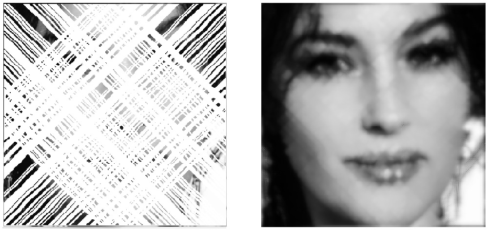
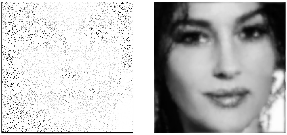
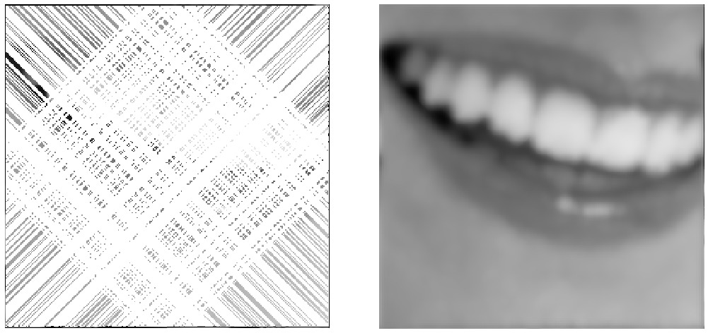
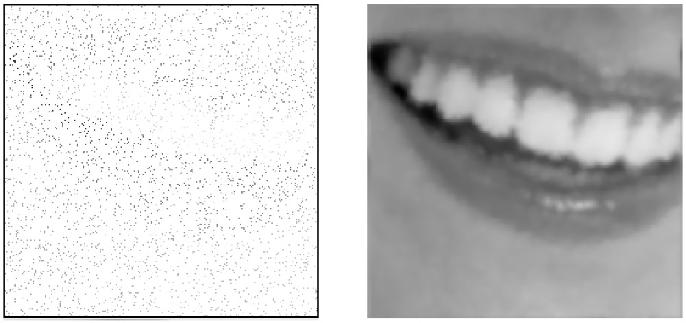
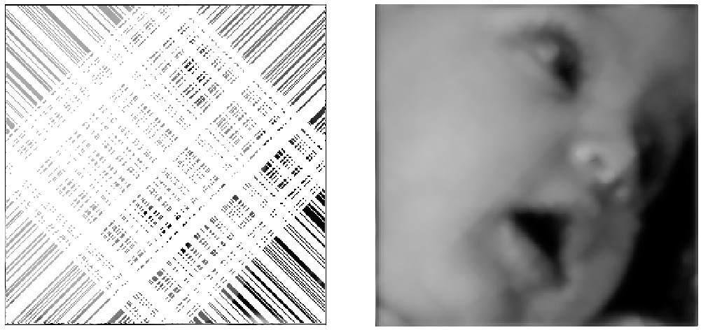
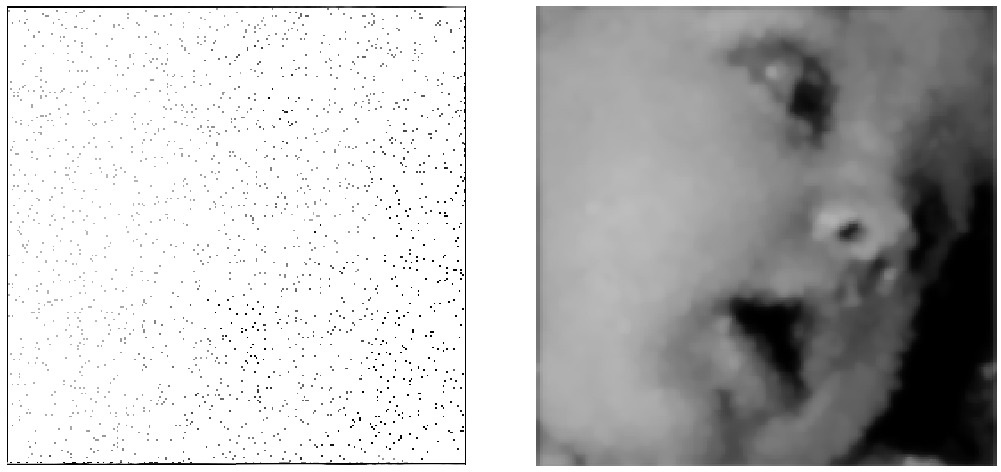
Figure 8: Images reconstructed with the AHE algorithm, Section 4. Two types of corruption are presented here. On the left: diagonal lines, total corruption is about 80%. On the right: uniform random distribution of corrupted pixels, total corruption is 90% (Bellucci), 95% (smile), 97% (child).

In practice, calculation of the slope angle $\theta(k,l)$ can have a large error appearing due to corrupted pixels, especially in the case of highly corrupted images (for instance, presented in Fig. 8). Therefore, it is important to know how does the distortion of this information affect the reconstruction. Section 2.4 contains a series of experimental results answering this question.

2.3.2 Projection

The final step of our algorithm is to convert the result of the evolution (4), denoted by

$$\overline{F}(x,y,\theta_{r})=\psi(x,y,\theta_{r},T)$$

into a function $F(x,y)$, which represents the reconstructed image. Observe that, due to the well-known properties of the (hypoelliptic) heat evolution, and the fact that the initial function $\overline{f}$ is non-negative, the same is true for $\psi$ at any time $t>0$. (See, e.g., Strichartz ; Strichartz-corr .)

A natural choice for this projection procedure is to consider the $\ell^{p}$-norm of the function $\overline{F}(x,y,\theta)$ with respect to $\theta\mod\pi$, where $1\leq p\leq\infty$. As discussed in Remizov2013 , we have chosen the $\ell^{\infty}$ norm. That is,

$$F(x_{k},y_{l})=\max_{\theta_{r}}\overline{F}(x_{k},y_{l},\theta_{r}).\\$$ (10)

After the projection, we obtain a non-negative function $F(x,y)$, whose maximal value, due to the action of the diffusion, is usually small. Therefore, it is necessary to renormalize:

$$F(x_{k},y_{l})\mapsto\frac{F(x_{k},y_{l})}{\max\limits_{k,l}F(x_{k},y_{l})}.$$

      

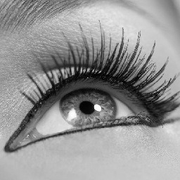
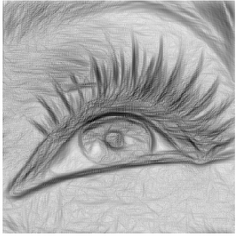
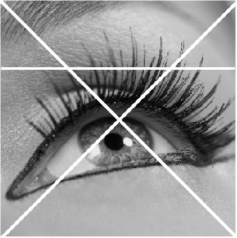
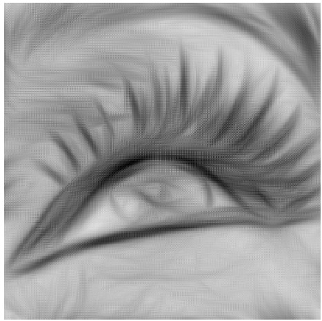
Figure 1: The evolution of the diffusion with different final times. The left pair presents the diffusion of non-corrupted image with small final time. The right pair presents the diffusion of slightly corrupted image with larger final time $T$ necessary for filling the white strips. In the both cases, the lift is done by (7)–(9)

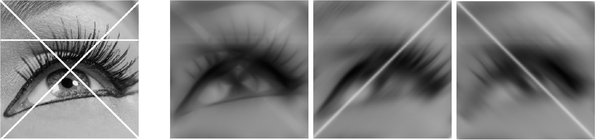
Figure 2: From the left to right: the corrupted image and three processed images showing the anisotropic nature of the diffusion. The lift is taken to be, respectively, the trivial one given by (9) at all points of the image, a lift with constant slope angle $\theta(k,l)\equiv\frac{\pi}{4}$ and a lift with constant slope angle $\theta(k,l)\equiv\frac{3\pi}{4}$.

      

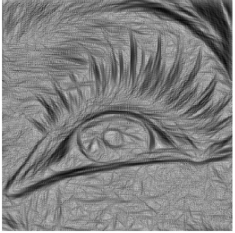
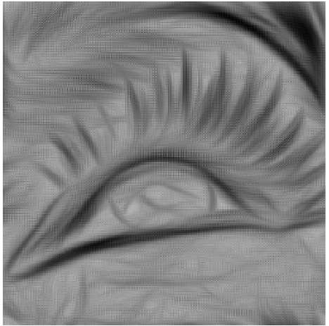
Figure 3: Two reconstructions showing the anisotropic nature of the diffusion. In both cases, the lift is done by formula (7), where the value $f(x_{k},y_{l})$ is replaced by the constant $\frac{1}{2}$. The left pair presents the diffusion of non-corrupted image with small final time. The right pair presents the diffusion of slightly corrupted image with larger final time $T$ necessary for filling the white strips.

2.4 Numerical experiments

In Fig. 1 to 3 we present some experimental results related to the above mentioned methods. They concern only the hypoelliptic evolution, without the SR/DR procedures discussed in the next section. As already mentioned, these experiments are done on images of size $256\times 256$ and $N=30$. No improvement is visible by choosing $N>30$.

• Fig. 1 presents the evolution of the diffusion in time. The initial image is lifted according to (7)–(9).

• Fig. 2 shows the anisotropic effect of the diffusion: The three processed images correspond to different kinds of lift. The first one is obtained with the trivial lift (9). The second processed image corresponds to a lift with the constant angle $\tfrac{\pi}{4}$ only, while the last one corresponds to a lift with the constant angle $\tfrac{3\pi}{4}$. Observe how in the two latter cases, the diffusion completely fills the white lines transversal to the fixed direction and preserves the one parallel to it.

• Fig. 3 illustrates the effect of the following perturbation of the lift: in (7) the slope angle $\theta_{r}\simeq\theta(k,l)$ is properly calculated by (8), but the true value $f(x_{k},y_{l})$ is replaced with a non-zero constant.

In Fig. 2 and 3 we show how modifying the lifting procedure alters the results of the diffusion, which however keeps its anisotropic character. Comparing these images with Fig. 1, one can see that the diffusion gives best results if the lift is obtained via (7)–(9). However, the trivial lift given only by (9) is useful when treating highly corrupted images, for which the precise evaluation of the gradient necessary to apply (7) is unachievable. Thus, in the following, we will always consider the trivial lift when the corruption is higher than $80\%$.

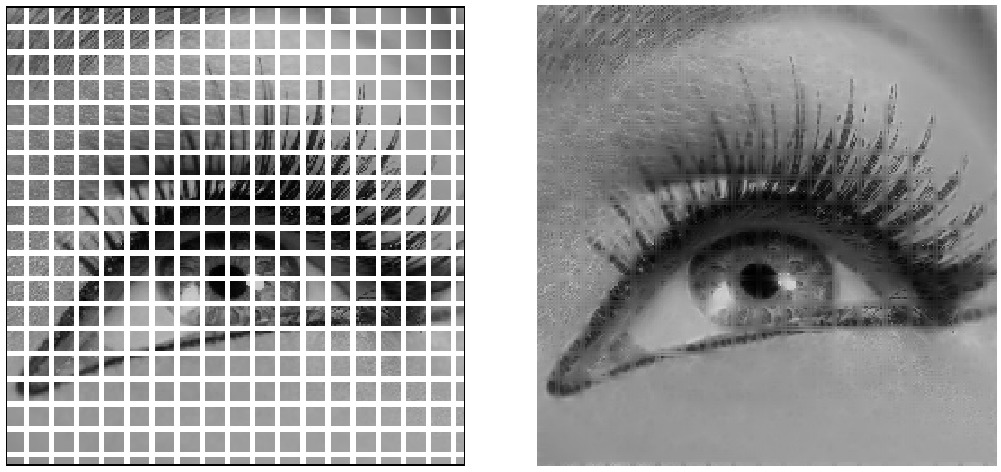
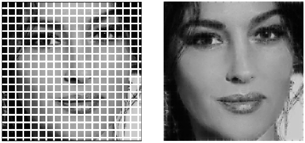
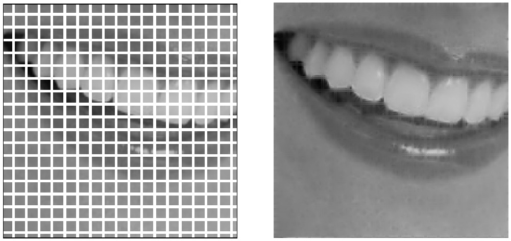
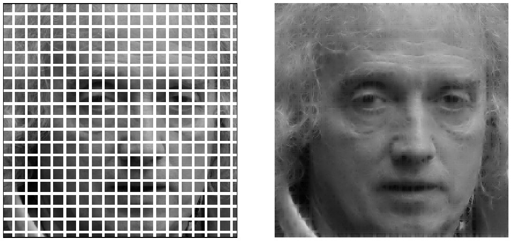
Figure 4: Images reconstructed with the hypoelliptic equation with varying coefficients and the DR procedure, Section 3. Total corruption: 37%, width of corrupted lines: 3 pixels.

2.5 Heuristic complements: SR/DR procedures

The above procedure has the drawback of applying the evolution to the whole image, and thus also on the non-corrupted part, blurring it. In Remizov2013 , we proposed an heuristic complement, allowing to keep track of the initial information during the evolution. This method is based upon the general idea of distinguishing between the so-called good and bad points (pixels) of the image under reconstruction. Roughly speaking, the set $G$ of good points consists of points that are already reconstructed enough (thus including non-corrupted points), while the set $B$ of bad points consists of points that are still corrupted. This procedure then amounts to slowing the effects of the diffusion on the set $G$, without influencing $B$. The idea of the restoration procedure is to “mix” the solution $\psi(x,y,\theta,t)$ of the diffusion equation with the initial function $\psi(x,y,\theta,0)={\overline{f}}(x,y,\theta)$ at each point $(x,y)\in G$.

In Remizov2013 , we described two possible realizations of this idea called static restoration (SR) and dynamic restoration (DR). The difference between the SR and the DR procedure consists in the way the sets of good and bad points are handled: in the SR procedure the set of good points $G$ coincides with the set of non-corrupted points and does not change during the diffusion, while in the DR procedure $G$ coincides with the set of non-corrupted points only initially and bad points are allowed to become good through the action of the diffusion.

An example of an image reconstructed with the DR procedure is given in Fig. 9(b). In Fig. 9(c) and (d), the same image is reconstructed with the more efficient methods presented in the following sections. As it will be explained later, the method used to obtain Fig. 9(c) is a combination of the DR procedure with the modified hypoelliptic diffusion presented in the next section.

3 A first improvement: Hypoelliptic diffusion with varying coefficients

One can try to modify equation (4) to take more into account the knowledge of the corrupted part of the image. A natural idea is to apply the diffusion only to corrupted regions of the image or to apply it with different final time $T$, larger at corrupted pixels and smaller at non-corrupted pixels. This approach requires the decomposition of the images into different domains with the subsequent reconciliation of the results of the diffusion. This scheme is very difficult to realize in practice. Therefore, we chose a different approach.

First, remark that the diffusion given by (4) has two parameters: the coefficient $\beta$ appearing in the operator $\Delta_{H}$ and the final time $T$. Obviously, the initial value problem (4) is equivalent to

$$\left\{\begin{aligned} &\frac{\partial\psi}{\partial t}=\Delta_{H}\psi,\ \ \,\Delta_{H}=a(X_{1})^{2}+b(X_{2})^{2},\\ &\psi\bigl{|}_{t=0}=\overline{f}(x,y,\theta),\\ \end{aligned}\right.$$ (11)

where the final time is equal to $1$, and the vector fields $X_{1}$, $X_{2}$ are defined in (3). Here $a,b$ are given by $a=T$ and $b=T\beta$.

Exploiting (11), we can control the intensity of the diffusion as a function of the position $(x,y)$, by considering $a,b$ as functions of $(x,y)$. Roughly speaking, we choose smaller values of $a,b$ at non-corrupted points and larger values at corrupted points.

The price we have to pay is the loss of the essential decoupling effect that allows to pass from (5) to the decoupled system (6). To overcome this point we use a well-known trick: at each step of integration we replace the varying coefficients equation (11) with a similar equation with constant coefficients. (See, e.g., (ferziger, , Chapter 6).) Namely, let $[t_{i},t_{i+1}]$ be the time interval of the integration and consider as initial datum the function $\psi_{i}:=\psi(x,y,\theta,t_{i})$ calculated at the previous step $[t_{i-1},t_{i}]$ (or the initial datum $\overline{f}$ if $t_{i}=0$).

Then, we replace the differential operator $\Delta_{H}$ on the interval $[t_{i},t_{i+1}]$ with the operator

$$\Delta^{\prime}_{H}:=a^{\prime}(X_{1})^{2}+b^{\prime}(X_{2})^{2},$$

where $a^{\prime},b^{\prime}$ are constant coefficients chosen, for instance, as $a^{\prime}=\max a(x,y)$, $b^{\prime}=\max b(x,y)$. The following approximation holds

$$\Delta_{H}\psi\approx\Delta^{\prime}_{H}\psi-\Delta^{\prime}_{H}\psi_{i}+\Delta_{H}\psi_{i}=\Delta^{\prime}_{H}\psi+d_{i},$$

where $d_{i}=\Delta_{H}\psi_{i}-\Delta^{\prime}_{H}\psi_{i}$ can be explicitly computed. Indeed, the approximate equality in the above formula become exact if $\psi_{i}$ is replaced with $\psi$, whence the approximation error is $\Delta(\psi_{i}-\psi)$, where $\Delta=\Delta_{H}-\Delta^{\prime}_{H}$, is small if $t_{i+1}-t_{i}$ is small enough.

Thus, on the interval $[t_{i},t_{i+1}]$ we replace equation (11) with the inhomogeneous equation

$$\frac{\partial\psi}{\partial t}=\Delta^{\prime}_{H}\psi+d_{i},\ \ \ t\in[t_{i},t_{i+1}],$$ (12)

with constant coefficients $a^{\prime},b^{\prime}$ and source $d_{i}$. After that, the decoupling effect mentioned in Section 2.2.3 persists and the semi-implicit method is still pertinent applied to each of the decoupled evolution equations, which differ from (6) only via $d_{i}$.

As already mentioned above, when choosing the varying coefficients $a,b$, the idea is to make them larger at bad points and their neighbors (especially the coefficient $a$, which has the most influence to the velocity of the diffusion). Since the bad points correspond to the set $f(x,y)=0$, the coefficients $a(x,y)$ and $b(x,y)$ can be chosen to be a continuous approximation of the indicator function of the set $\{f(x,y)=0\}$. The continuity is desirable for better stability of the numerical integration. For instance, we consider the following simple formula for the coefficients:

$$\begin{split}a(x,y)&=a_{0}+a_{1}\exp\biggl{(}-\frac{f^{2}(x,y)}{\sigma}\biggr{)},\\ b(x,y)&=b_{0}+b_{1}\exp\biggl{(}-\frac{f^{2}(x,y)}{\sigma}\biggr{)},\end{split}$$ (13)

where $a_{i},b_{i},\sigma$ are positive constant parameters chosen experimentally.

3.1 Numerical experiments

In Fig. 4, we present a series of reconstructions obtained with the diffusion (11) with varying coefficients coupled with the DR procedure and using the trivial lift, i.e., the lift defined by (9) at all points of the image. The coefficients of the diffusion are defined by (13) with parameters $a_{0}=0.1,\ a_{1}=0.4$, $b_{0}=1.1,\ b_{1}=10$,  $\sigma=0.1$.

In Fig. 9, we present a comparison of an image reconstructed with this method, Fig. 9(c), with the methods presented in the previous section, Fig. 9(b), and with the final algorithm, Fig. 9(d), presented in the next section.

4 AHE algorithm

In this section we present the main subject of this paper: the Averaging and Hypoelliptic Evolution (AHE) algorithm. The main idea behind the AHE algorithm is to provide the anisotropic diffusion with better initial conditions. More precisely, it is divided in the following 4 steps:

1. Preprocessing phase (Simple averaging);

2. Main diffusion (Strong smoothing);

3. Advanced averaging;

4. Weak smoothing.

Let us denote the sets of good and bad points by respectively $G$ and $B$. Initially (before starting the algorithm) these sets are

$$\begin{split}G&=\{(x_{k},y_{l})\mid f(x_{k},y_{l})>0\},\\ B&=\{(x_{k},y_{l})\mid f(x_{k},y_{l})=0\},\end{split}$$

Observe that $B\cup G$ covers the whole image (the whole grid) and neither $B$ nor $G$ are empty. For each $(x_{k},y_{l})\in B$ denote by $\Theta_{kl}$ its 9-points neighborhood. Define the set $G_{kl}=G\cap\Theta_{kl}$ and let $|G_{kl}|$ be the cardinality of $G_{kl}$. Obviously, $0\leq|G_{kl}|\leq 8$. We call $\partial B$ the set of boundary bad points, i.e., of those $(x_{k},y_{l})\in B$ satisfying the condition $|G_{kl}|>0$.

Remark 1

The AHE algorithm includes the hypoelliptic diffusion with the varying coefficients presented in Section 3 (steps 2 and 4). At the both steps, the diffusion can be performed either with the SR/DR procedure or without it. Numerous experiments show that using the SR/DR procedure allows to slightly improve the quality of reconstruction if the cardinality of the set $G$ (the number of non-corrupted pixels) is large enough. However, in the case of highly corrupted images (such as those presented in Fig. 7, 8) using the SR/DR procedure gives almost no significant improvement. For this reason, in the following we use the diffusion without the SR/DR procedure.

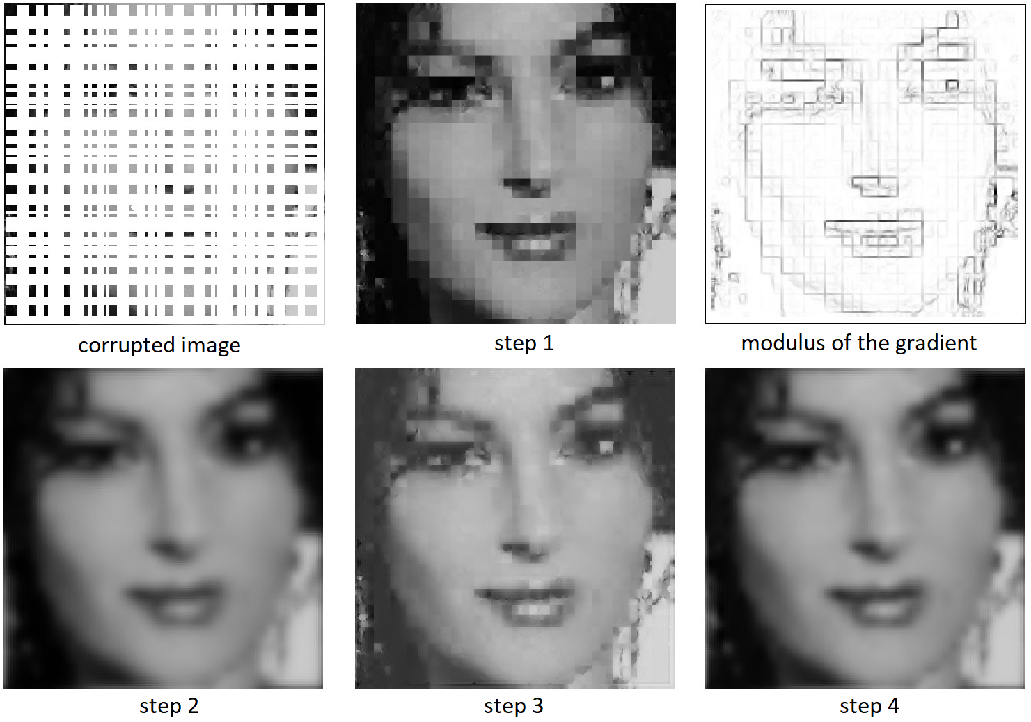
Figure 5: The result of reconstruction obtained after each of four steps in the AHE algorithm. The third image depicts the modulus of the gradient of the result of step 1, which we use to compute the varying coefficients in step 2.

4.1 Step 1: Preprocessing phase (Simple averaging)

The aim of this phase is to fill in the corrupted areas of the picture with a rough approximation of what the reconstruction should be, obtained via a discrete approximation of an isotropic diffusion. Namely, we iteratively redefine the value of $f$ at each boundary bad point $(x_{k},y_{l})$ to be the average value of the good points in its 9-points neighborhood $\Theta_{kl}$. Then, we remove $(x_{k},y_{l})$ from $B$ and add it to $G$.

More precisely, let $f^{0}=f$, $G^{0}=G$ and $B^{0}=B$. Given $f^{i}$, $G^{i}$ and $B^{i}$ we define $f^{i+1}$, $G^{i+1}$ and $B^{i+1}$ as follows. For any $(x_{k},y_{l})\in\partial B^{i}$ we put

$$f^{i+1}(x_{k},y_{l})={\frac{1}{|G^{i}_{kl}|}\sum_{(x,y)\in G^{i}_{kl}}}f^{i}(x,y),$$ (14)

and for any $(x_{k},y_{l})\notin\partial B^{i}$ we put

$$f^{i+1}(x_{k},y_{l})=f^{i}(x_{k},y_{l}).$$

Observe, in particular, that this formula leaves the values of $f^{i+1}$ on $B^{i}\setminus\partial B^{i}$ to be zero. Finally, we let $G^{i+1}=G^{i}\cup\partial B^{i}$ and $B^{i+1}=B^{i}\setminus\partial B^{i}$.

Since the set $\partial B^{i}=\emptyset$ if and only if $B^{i}=\emptyset$, after a finite number of step $s$ we obtain $B^{s}=\emptyset$. We then let $g=f^{s}$ to be the result of this procedure. Observe that, in particular, $g(x_{k},y_{l})>0$ for all $(x_{k},y_{l})$.

4.2 Step 2: Main diffusion (Strong smoothing)

The goal of this step is the elimination (or at least weakening) of the “mosaic” effect resulting from the previous step. Here, we apply diffusion (11) with varying coefficients $a,b$ chosen so that the diffusion is more intensive at the points where the “mosaic” effect is more strong. To estimate the intensity of the “mosaic” effect, we use the absolute value of the gradient of the function $g$. Indeed, comparing the images presented in Fig. 5, one can see that most of the points with strong “mosaic” effect coincide with the points where $|\nabla g(x,y)|$ is large.

Thus, we apply the hypoelliptic diffusion (11) with initial condition $\overline{g}(x,y,\theta)$, obtained from $g(x,y)$ by the trivial lift (9) at all points. The choice of the trivial lift has an obvious advantage if we deal with highly corrupted images: if we were using (7) – (9), the most important contribution would not be given by the contours of the image, but by the boundaries of the “mosaic” effect. This would force the diffusion to follow such boundaries (see the results presented in Fig. 2), thus preventing the smoothing effect.

As already mentioned above, we control the intensities of diffusion (11) via the varying coefficients $a(x,y)$, $b(x,y)$, which can be defined by a formula similar to (13) with an obvious difference: while the coefficients (13) correspond to slowing down the diffusion at points with large values of $f(x,y)$, now we need to slow down the diffusion at points with small values of $|\nabla g(x,y)|$. For instance,

$$\begin{split}a(x,y)=a_{0}+a_{1}\exp\biggl{(}-\frac{\varphi^{2}(x,y)}{\sigma}\biggr{)},\\ b(x,y)=b_{0}+b_{1}\exp\biggl{(}-\frac{\varphi^{2}(x,y)}{\sigma}\biggr{)},\\ \end{split}$$ (15)

where

$$\varphi(x,y)=1-\frac{|\nabla g(x,y)|}{\max\limits|\nabla g(x,y)|}.$$

Here, $a_{i},b_{i},\sigma$ are constant parameters experimentally chosen. In all restorations via the AHE algorithm presented in this paper, we used the following values of the parameters: $a_{0}=0.05$, $a_{1}=0.2$, $b_{0}=0.55$, $b_{1}=5$, $\sigma=0.4$. From the practical point of view, the gradient $\nabla g(x,y)$ is replaced by its finite-difference approximation.

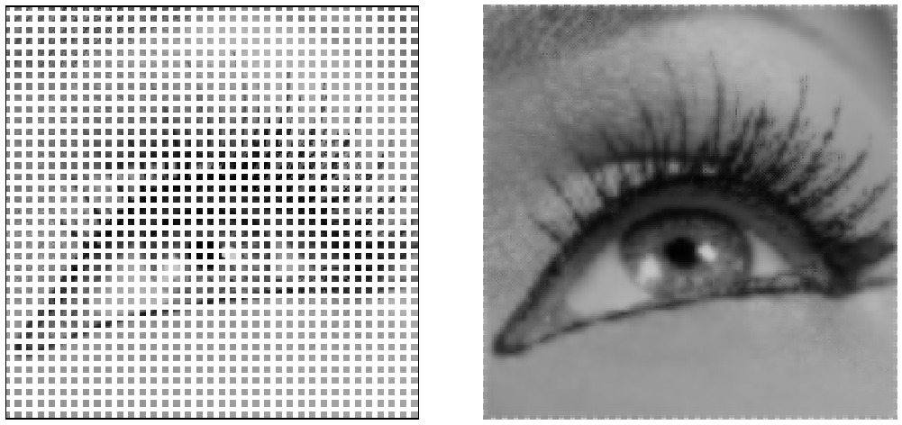
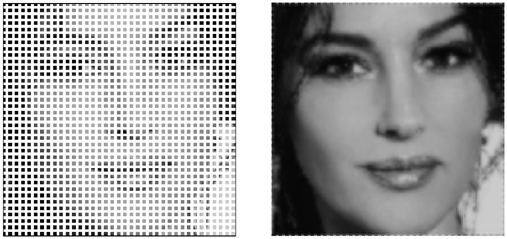
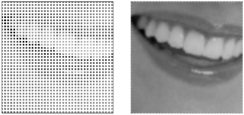
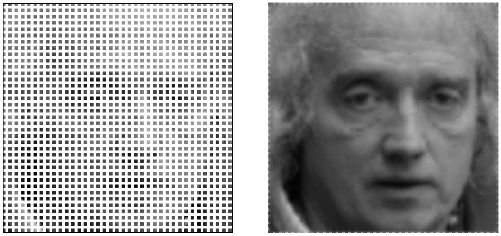
Figure 6: Images reconstructed with the AHE algorithm, Section 4. Total corruption: 67%, width of corrupted lines: 3 pixels.

4.3 Step 3: Synthesis (Advanced averaging)

As can be seen in Fig. 5, after the second step of the AHE algorithm we remove the “mosaic” effect. However, the diffusion introduces a blurring effect, that cannot be removed by decreasing the coefficients $a,b$, since these have to be sufficiently large in order to remove the “mosaic” effect. To pass between this Scylla and Charybdis, we then make a synthesis of the images obtained after the first and the second steps.

As before, let $f(x,y)$ be the function of the initial corrupted image, and $B,G$ be the corresponding sets of good and bad points. Recall that we denoted by $g(x,y)$ the function obtained after the first step and let $h(x,y)$ denote the function obtained after the second step.

The structure of step 3 is similar to the one of step 1. Indeed, we will apply an iterative procedure aimed to reconstruct the bad points of $f$ using information from the good points and the function $h$. The only difference between steps 1 and 3 is that when $(x_{k},y_{l})\in\partial B^{i}$, we define $f^{i+1}(x_{k},y_{l})$ as

$$f^{i+1}(x_{k},y_{l})=\arg\min_{X\in[0,1]}\sum_{(x,y)\in G^{i}_{kl}}\biggl{|}\frac{X}{f^{i}(x,y)}-\frac{h(x_{k},y_{l})}{h(x,y)}\biggr{|}^{2}.$$ (16)

This expression realizes a compromise between the averaging and the diffusion. The above formula is well defined since $f(x,y)>0$ for all $(x,y)\in G^{i}_{kl}$ and the smoothed function $h(x,y)$ is always strictly positive. Moreover, the expression in the right-hand side of (16) is a continuous convex function of $X$, and thus the minimum exists. A straightforward computation allows then to compute explicitly (16) as

$$f^{i+1}(x_{k},y_{l})=h(x_{k},y_{l})\,\frac{\sum\limits_{(x,y)\in G^{i}_{kl}}f^{i}(x,y)^{-1}h(x,y)^{-1}}{\sum\limits_{(x,y)\in G^{i}_{kl}}f^{i}(x,y)^{-2}}.$$

The results of this reconstruction are presented in Fig. 5. As desired, we obtain a somewhat intermediate result, between step 1 and step 2.

4.4 Step 4: Weak smoothing

As can be seen from Fig. 5, step 3 also reintroduces “mosaic” effect, but less than step 1. Therefore, we essentially need to repeat step 2. The only difference is that the parameters $a_{i},b_{i}$ in (15) should be chosen smaller than those in step 2.

In all reconstructed images presented in Fig. 6 – 8 we use the trivial lift (9) and hypoelliptic diffusion (11) with varying coefficients $a,b$ defined by (15). For the results presented in Fig. 7, 8, we used the following parameters: $a_{0}=0.015$, $a_{1}=0.1$, $b_{0}=0.15$, $b_{1}=1.5$, $\sigma=0.3$.

4.5 Numerical cost of the algorithm

Computational cost of the AHE algorithm is moderate. Let us consider an input image of size $M\times M$ pixels and $N$ possible directions. The most computationally expensive part is the hypoelliptic diffusion with varying coefficients, which appears in the AHE algorithm twice (steps 2, 4).

At each time step, the hypoelliptic diffusion is represented by a system of $M^{2}$ linear inhomogeneous evolution equations. Each of them is solved using the Crank-Nicolson scheme (see, e.g., Marchuk1982 ), which requires to solve a system of linear algebraic equations with a $N\times N$ periodic tridiagonal matrix. This can be done in $O(N)$ operations via a variation of Thomas algorithm. Thus, taking into account the two-dimensional Fast Fourier Transforms (FFTs) necessary to decouple the system, which require $O(M^{2}\log M)$ operations each, the total computational cost per time step is

$$O(NM^{2}+NM^{2}\log M)=O(NM^{2}\log M).$$

The run-time of the sequential implementation of the AHE algorithm used to perform the reconstructions presented in this paper is of about two minutes. The code has been run on an Intel i7-4600M CPU, with parameters $M=256$ and $N=32$. We remark that the systems of $M^{2}$ linear inhomogeneous evolution equations are completely decoupled, as are the two-dimensional FFTs. This can be exploited to develop a parallel implementation, allowing for a significant reduction of the run-time.

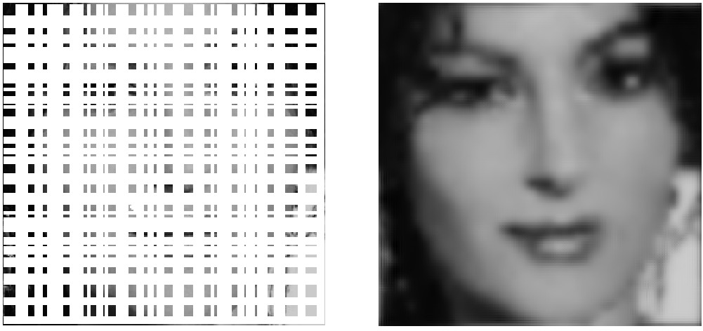
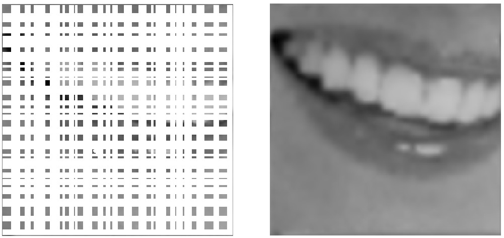
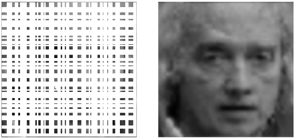
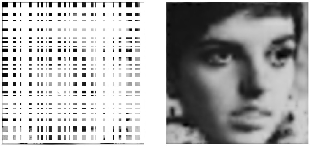
Figure 7: Images reconstructed with the AHE algorithm, Section 4. Total corruption: 85%.

5 Conclusion

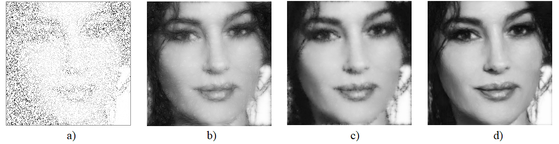
Figure 9: A comparison of reconstructions of an image with $80\%$ of pixels missing. a) the original corrupted image. b) Reconstruction with the DR method and the hypoelliptic diffusion presented in Section 2. See also Remizov2013 . c) Reconstruction with the DR procedure and the varying coefficient hypoelliptic diffusion presented in Section 3. d) reconstruction with the AHE algorithm.

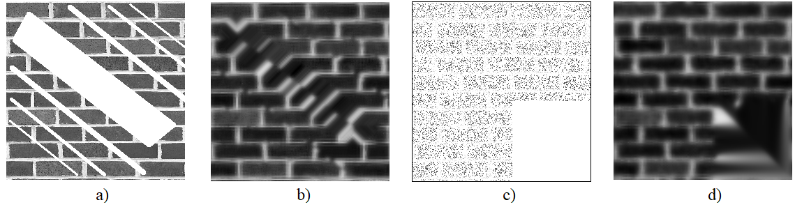
Figure 10: a) Image containing small and large corrupted regions. b) Reconstruction by the AHE algorithm. c) Image containing uniformly random corruption and a single large corrupted region. d) Reconstruction by the AHE algorithm.

The AHE algorithm presented in the paper, provides an efficient method of reconstruction for greyscale images, including highly corrupted ones. A comparison with the other methods presented in this paper is pictured in Fig. 9. We stress that this inpainting technique can be applied independently of the structure and the geometry of the corruption, although it requires the precise knowledge of its location. The quality of reconstruction strongly depends on the accuracy of this information.

Notice that the effectiveness of the algorithm depends also on the distribution of the corrupted pixels. Fig. 6–8 show that if the corruption is “well distributed” one can achieve good reconstructions even in presence of 97% pixels missing. However, if the image contains large corrupted regions, then the reconstructions are no longer satisfactory. To this effect, see Fig. 10.

It seems obvious that the AHE algorithm is open to further development. For instance, the first step (simple averaging) can be replaced with a more advanced method. Also, the detection of the regions presenting a “mosaic” effect is currently done in a very naive way, via (15). Moreover, the coefficients $a_{i},b_{i}$ and $\sigma$ appearing in that equation have been determined experimentally and their choice can clearly be optimized. This step could be done, for example, via image recognition methods based on the semi-discrete group of rototranslations PrandiBohi ; PBG2015 .

Appendix A Sub-Riemannian geometry

In this Appendix we recall some standard definitions of sub-Riemannian geometry and hypoelliptic operators. Classical texts are montgomery ; nostrolibro ; bellaiche ; gromov .

Definition 1

A $(n,m)$-sub-Riemannian manifold is given by a triple $(M,{\blacktriangle},{\mathbf{g}})$, where

• $M$ is a connected smooth manifold of dimension $n$;

• ${\blacktriangle}$ is a smooth distribution of constant rank $m<n$ satisfying the Hörmander condition. That is, ${\blacktriangle}$ is a smooth map that associates to $q\in M$ an $m$-dimensional subspace ${\blacktriangle}(q)$ of $T_{q}M$, such that $\forall\leavevmode\nobreak\ q\in M$ we have

  $$T_{q}M={\operatorname{span}}\{[X_{1},[\ldots[X_{k-1},X_{k}]]](q)\leavevmode\nobreak\ |\leavevmode\nobreak\ X_{i}\in\mathrm{Vec}_{H}(M)\}.$$ (17)

  Here, $\mathrm{Vec}_{H}(M)$ denotes the set of horizontal smooth vector fields on $M$, i.e.

  $$\mathrm{Vec}_{H}(M)=\{X\in\mathrm{Vec}(M)\ |\ X(q)\in{\blacktriangle}(q)\leavevmode\nobreak\ \ \forall\leavevmode\nobreak\ q\in M\}.$$

• ${\mathbf{g}}_{q}$ is a Riemannian metric on ${\blacktriangle}(q)$, smooth as function of $q$.

A Lipschitz continuous curve $q(\cdot):[0,T]\to M$ is said to be horizontal if $\dot{q}(t)\in{\blacktriangle}(q(t))$ for almost every $t\in[0,T]$. Given an horizontal curve $q(\cdot):[0,T]\to M$, the length of $q(\cdot)$ is

$$\ell(q(\cdot))=\int_{0}^{T}\sqrt{{\mathbf{g}}_{q(t)}(\dot{q}(t),\dot{q}(t))}\leavevmode\nobreak\ dt.$$ (18)

The distance induced by the sub-Riemannian structure on $M$ is the function

$$d(q_{0},q_{1})=\inf\{\ell(q(\cdot))\mid q(0)=q_{0},q(T)=q_{1},q(\cdot)\ \mathrm{horizontal}\}.$$ (19)

The connectedness assumption for M and the Hörmander condition guarantee the finiteness and the continuity of $d(\cdot,\cdot)$ with respect to the topology of $M$ (Chow’s Theorem, see for instance nostrolibro ). The function $d(\cdot,\cdot)$ is called the Carnot-Carathéodory distance and gives to $M$ the structure of metric space.

Locally, the pair $({\blacktriangle},{\mathbf{g}})$ can be specified by assigning a set of $m$ smooth vector fields spanning ${\blacktriangle}$, that are moreover orthonormal for ${\mathbf{g}}$, i.e.

$${\blacktriangle}(q)={\operatorname{span}}\{X_{1}(q),\dots,X_{m}(q)\},\leavevmode\nobreak\ \leavevmode\nobreak\ \leavevmode\nobreak\ {\mathbf{g}}_{q}(X_{i}(q),X_{j}(q))=\delta_{ij}.$$ (20)

Such a set $\{X_{1},\ldots,X_{m}\}$ is called a local orthonormal frame for the sub-Riemannian structure. When $({\blacktriangle},{\mathbf{g}})$ can be defined by $m$ globally defined vector fields as in (20) we say that the sub-Riemannian manifold is trivializable.

Given a trivializable $(n,m)$-sub-Riemannian manifold, the problem of finding a curve realizing the distance between two fixed points $q_{0},q_{1}\in M$ is naturally formulated as the following optimal control problem

$$\left\{\begin{aligned} \phantom{o}&\dot{q}(t)=\sum_{i=1}^{m}u_{i}(t)X_{i}(q(t)),\ \ u_{i}(\cdot)\in L^{\infty}([0,T],{\mathbb{R}}),\\ \phantom{o}&\int\limits_{0}^{T}\sqrt{\sum_{i=1}^{m}u_{i}^{2}(t)}\leavevmode\nobreak\ dt\,\to\,\min,\\ \phantom{o}&q(0)=q_{0},\ \ \ q(T)=q_{1}.\\ \end{aligned}\right.$$ (21)

A.1 Diffusion in a sub-Riemannian manifold

Given a sub-Riemannian manifold $(M,{\blacktriangle},{\mathbf{g}})$ and a smooth volume $\omega$ on $M$, the sub-Riemannian heat equation is the diffusion equation:

$$\partial_{t}\psi=\Delta_{H}\psi,$$ (22)

where $\Delta_{H}$ is the sub-Riemannian (or horizontal) Laplacian, defined by

$$\Delta_{H}\varphi=\operatorname{div}_{\omega}\operatorname{grad}_{H}\varphi,\qquad\varphi\in C^{2}(M).$$ (23)

Here, $\operatorname{div}_{\omega}$ is the divergence with respect to the volume $\omega$ and $\operatorname{grad}_{H}\varphi$ is the horizontal gradient of $\varphi$. That is, it is the unique vector field satisfying, for every $q\in M$,

$${\mathbf{g}_{q}}(\operatorname{grad}_{H}\varphi(q),v)=d_{q}\varphi(v)\mbox{ for every }v\in{\blacktriangle}(q).$$ (24)

If $\{X_{1},\ldots,X_{m}\}$ is a local orthonormal frame, it follows that $\operatorname{grad}_{H}\varphi=\sum_{i=1}^{m}(X_{i}\varphi)X_{i}$, and thus that

$$\Delta_{H}\varphi=\sum_{i=1}^{m}\left(X_{i}^{2}\varphi+(\operatorname{div}_{\omega}X_{i})X_{i}\varphi\right).$$ (25)

Thanks to the Hörmander condition assumed in the definition of the sub-Riemannian manifold, the celebrated Hörmander Theorem Hormander , implies the following.

Theorem A.1

The operators $\Delta_{H}$ (operating on functions $\varphi:M\to{\mathbb{R}}$) and $\Delta_{H}-\partial_{t}$ (operating on functions $\psi:M\times{\mathbb{R}}\to{\mathbb{R}}$) are hypoelliptic.

We recall that a second order differential operator $L$ is said to be hypoelliptic if for every distribution $\varphi$ defined on an open set $\Omega$ of a manifold $N$, the condition $L\varphi\in{C}^{\infty}(\Omega)$ implies that $\varphi\in{C}^{\infty}(\Omega)$. In particular, the hypoellipticity of $\Delta_{H}-\partial_{t}$ implies that any solution to the heat equation (22) on $M\times]t_{0},t_{1}[$ is smooth.

Remark 2

The sub-Riemannian structure studied in this paper is the one on $PT{\mathbb{R}}^{2}$ for which the distribution is given by the vector fields

$$X_{1}(q)=\cos\theta\frac{\partial}{\partial x}+\sin\theta\frac{\partial}{\partial y},\ \ \ X_{2}(q)=\frac{\partial}{\partial\theta}.$$ (26)

The metric $\mathbf{g}$ is then chosen such that $\{X_{1},X_{2}\}$ are orthogonal, and ${\mathbf{g}}(X_{1},X_{1})=1$, ${\mathbf{g}}(X_{2},X_{2})=1/\beta$, for some given $\beta>0$. By taking as volume on $PT{\mathbb{R}}^{2}$ the Lebesgue measure, i.e., $\omega=dx\,dy\,d\theta$, since $X_{1}$ and $X_{2}$ are divergence free, one immediately gets

$$\Delta_{H}=(X_{1})^{2}+\beta(X_{2})^{2}.$$

References

- (1) F. Abas. Analysis of craquelure patterns for content-based retrieval. PhD thesis, University of Southampton, 2004.
- (2) A. Agrachev, D. Barilari, and U. Boscain. Introduction to Riemannian and sub-Riemannian geometry (Lecture Notes). http://webusers.imj-prg.fr/~davide.barilari/notes.php.
- (3) A. Bellaïche. The tangent space in sub-Riemannian geometry. In Sub-Riemannian geometry, volume 144 of Progr. Math., pages 1–78. Birkhäuser, Basel, 1996.
- (4) M. Bertalmio, G. Sapiro, V. Caselles, and C. Ballester. Image inpainting. In Proc. of SIGGRAPH 2000, New Orleans, USA, pages 417–424, 2000.
- (5) A. Bohi, D. Prandi, V. Guis, F. Bouchara, and J.-P. Gauthier. Fourier descriptors based on the structure of the human primary visual cortex with applications to object recognition. J. Math. Imaging Vision, 57(1):117–133, 2017.
- (6) U. Boscain, G. Charlot, and F. Rossi. Existence of planar curves minimizing length and curvature. Proc. Steklov Inst. Math., 270:43–56, 2010.
- (7) U. Boscain, R.A. Chertovskih, J.-P. Gauthier, and A.O. Remizov. Hypoelliptic diffusion and human vision: a semidiscrete new twist. SIAM J. Imaging Sci., 7(2):669–695, 2014.
- (8) U. Boscain, R. Duits, F. Rossi, and Yu. Sachkov. Curve cuspless reconstruction via sub-Riemannian geometry. ESAIM Control Optim. Calc. Var., 20(3):748–770, 2014.
- (9) U. Boscain, J. Duplaix, J.-P. Gauthier, and F. Rossi. Anthropomorphic image reconstruction via hypoelliptic diffusion. SIAM J. Control Optim., 50(3):1–25, 2012.
- (10) U. Boscain, J.-P. Gauthier, D. Prandi, and A. Remizov. Image reconstruction via non-isotropic diffusion in Dubins/Reed-Shepp-like control systems. In 53rd IEEE Conference on Decision and Control, pages 4278–4283, 2014.
- (11) A. Bugeau, M. Bertalmío, V. Caselles, and G. Sapiro. A comprehensive framework for image inpainting. IEEE Trans. Image Process., 19(10):2634–45, 2010.
- (12) T.F. Chan, S.H. Kang, and J. Shen. Euler’s elastica and curvature-based inpainting. SIAM J. Appl. Math., 63(2):564–592, 2002.
- (13) G. Citti, B. Franceschiello, G. Sanguinetti, and A. Sarti. Sub-Riemannian mean curvature flow for image processing. SIAM J. Imaging Sci., 9(1):212–237, 2016.
- (14) G. Citti and A. Sarti. A cortical based model of perceptual completion in the roto-translation space. J. Math. Imaging Vis., 24(3):307–326, 2006.
- (15) B. Cornelis, T. Ružić, E. Gezels, A. Dooms, A. Pižurica, L. Platiša, J. Cornelis, M. Martens, M. De Mey, and I. Daubechies. Crack detection and inpainting for virtual restoration of paintings: The case of the ghent altarpiece. Signal Processing, 93(3):605–619, 2013.
- (16) R. Duits, U. Boscain, F. Rossi, and Y. Sachkov. Association fields via cuspless sub-Riemannian geodesics in SE(2). J. Math. Imaging Vision, 49(2):384–417, 2014.
- (17) R. Duits and E. Franken. Left-invariant parabolic evolutions on and contour enhancement via invertible orientation scores Part I: linear left-invariant diffusion equations on . Quart. Appl. Math., 68(2):255–292, 2010.
- (18) R. Duits and E. Franken. Left-invariant parabolic evolutions on and contour enhancement via invertible orientation scores Part II: nonlinear left-invariant diffusions on invertible orientation scores. Quart. Appl. Math., 68(2):293–331, 2010.
- (19) R. Duits and M.A. van Almsick. The explicit solutions of linear left-invariant second order stochastic evolution equations on the 2D euclidean motion group. Quart. Appl. Math., 66:27–67, 2008.
- (20) G. Facciolo, P. Arias, V. Caselles, and G. Sapiro. Exemplar-based interpolation of sparsely sampled images. In D. Cremers, Yu. Boykov, A. Blake, and F.R. Schmidt, editors, Energy Minimization Methods in Computer Vision and Pattern Recognition: 7th International Conference EMMCVPR 2009 (Bonn, Germany, August 24–27, 2009) Proceedings, pages 331–344. Springer, 2009.
- (21) J.H. Ferziger and M. Perić. Computational methods for fluid dynamics. Berlin: Springer, 3rd rev. edition, 2002.
- (22) M. Gromov. Carnot-Carathéodory spaces seen from within. In Sub-Riemannian geometry, volume 144 of Progr. Math., pages 79–323. Birkhäuser, Basel, 1996.
- (23) R.K. Hladky and S.D. Pauls. Minimal surfaces in the roto-translation group with applications to a neuro-biological image completion model. J. Math. Imaging Vision, 36(1):1–27, 2010.
- (24) L. Hörmander. Hypoelliptic second order differential equations. Acta Math., 119:147–171, 1967.
- (25) D.H. Hubel and T.N. Wiesel. Receptive fields of single neurones in the cat’s striate cortex. J. Physiol., 148:574–591, 1959.
- (26) G.I. Marchuk. Methods of Numerical Mathematics. Springer, 1982.
- (27) D. Marr and E. Hildreth. Theory of edge detection. Proc. R. Soc. Lond. B. Biol. Sci., 207(1167):187–217, 1980.
- (28) S. Masnou. Disocclusion: a variational approach using level lines. IEEE Trans. Image Process., 11(2):68–76, 2002.
- (29) S. Masnou and J.-M. Morel. Level lines based disocclusion. In Proc. 5th IEEE Int. Conf. on Image Processing, pages 259–263 vol. 3, 1998.
- (30) R. Montgomery. A tour of subriemannian geometries, their geodesics and applications, volume 91 of Mathematical Surveys and Monographs. American Mathematical Society, Providence, RI, 2002.
- (31) L. Peichl and H. Wässle. Size, scatter and coverage of ganglion cell receptive field centres in the cat retina. J. Physiol., 291:117–141, 1979.
- (32) J. Petitot. The neurogeometry of pinwheels as a sub-Riemannian contact structure. J. Physiol. Paris, 97(2-3):265–309, 2003.
- (33) J. Petitot. Neurogéométrie de la vision - Modèles mathématiques et physiques des architectures fonctionnelles. Les Éditions de l’École Polytechnique, 2008.
- (34) N. Ponomarenko, L. Jin, V. Lukin, and K. Egiazarian. Self-similarity measure for assessment of image visual quality. In Proceedings of the 13th International Conference on Advanced Concepts for Intelligent Vision Systems, ACIVS’11, pages 459–470, Berlin, Heidelberg, 2011. Springer-Verlag.
- (35) D. Prandi, U. Boscain, and J.-P. Gauthier. Image processing in the semidiscrete group of rototranslations. In Geometric science of information, volume 9389 of Lecture Notes in Comput. Sci., pages 627–634. Springer, 2015.
- (36) D. Prandi and J.-P. Gauthier. A semidiscrete version of the Petitot model as a plausible model for anthropomorphic image reconstruction and pattern recognition. SpringerBriefs in Mathematics. Springer, To appear.
- (37) G. Sanguinetti, G. Citti, and A. Sarti. Image completion using a diffusion driven mean curvature flow in a sub-Riemannian space. In Proceedings of the 3rd International Conference on Computer Vision Theory and Applications (VISAPP 2008), volume 2, pages 46–53, 2008.
- (38) R. S. Strichartz. Sub-Riemannian geometry. J. Differential Geom., 24(2):221–263, 1986.
- (39) R. S. Strichartz. Corrections to: “Sub-Riemannian geometry” [J. Differential Geom. 24 (1986), no. 2, 221–263; MR0862049 (88b:53055)]. J. Differential Geom., 30(2):595–596, 1989.
- (40) V.V. Voronin, V.A. Frantc, V.I. Marchuk, A.I. Sherstobitov, and K. Egiazarian. No-reference visual quality assessment for image inpainting. In Proc. SPIE 9399, Image Processing: Algorithms and Systems XIII, 93990U (March 16, 2015), page 93990U, 2015.
- (41) M. Wang, B. Yan, and K.N. Ngan. An efficient framework for image/video inpainting. Signal Process. Image Commun., 28(7):753–762, 2013.
- (42) F. Zhang, S. Li, L. Ma, and K.N. Ngan. Limitation and challenges of image quality measurement. In Proc. SPIE 7744, Visual Communications and Image Processing 2010, 774402 (July 13, 2010), pages 774402–774402–8, 2010.