Thermal Corrections to Entanglement Entropy from Holography

Abstract

We use holographic techniques to calculate the first thermal correction to the entanglement entropy of a cap-like region of a CFT defined on a sphere, successfully reproducing the field theory result. Since this is an order-one correction to the entropy in the large-$N$ expansion, quantum corrections to the holographic entanglement entropy formula are essential. The bulk calculation is made tractable using the same technical machinery recently used to derive the linearized Einstein equations in the bulk from the first law of entanglement entropy in the CFT.

1 Introduction

Herzog Herzog:2014fra has recently calculated the first thermal correcton to the entanglement entropy of a cap-like region $B$ for a CFT defined on $R\times S^{d-1}$. The CFT is assumed to have a mass gap $\Delta$ and degeneracy $g$ in the first excited state, in terms of which we have

$$\delta S^{\rm CFT}_{B}(T)\equiv S_{B}(T)-S_{B}(0)=g\Delta e^{-\beta\Delta}I_{d}(\theta_{0})+o(e^{-\beta\Delta})$$ (1)

where

$$I_{d}(\theta_{0})=2\pi\frac{\Omega_{d-2}}{\Omega_{d-1}}\int_{0}^{\theta_{0}}d\theta\frac{\cos\theta-\cos\theta_{0}}{\sin\theta_{0}}\sin^{d-2}\theta,$$ (2)

the opening angle of the cap is $2\theta_{0}$, $\Omega_{d-1}$ is the volume of $S^{d-1}$, and the CFT is at temperature $T=\beta^{-1}$. We are working in units where the sphere has radius one.

The result (1) is independent of $N$ in the sense of large-$N$ CFTs, and so in the large-$N$ expansion should appear at $O(1)$. To calculate $O(1)$ corrections to the entropy holographically, we need to use the quantum generalization of the Ryu-Takayanagi Ryu:2006bv entropy formula due to Faulkner, Lewkowycz, and Maldacena Faulkner:2013ana :

$$S=\frac{A}{4G_{N}}+S_{\rm bulk},$$ (3)

where $A$ is the area of the extremal surface anchored on the boundary of $B$ and $S_{\rm bulk}$ is the entanglement entropy of the bulk matter in the region between $B$ and the extremal surface. We will also note that, in finding the difference between the $T=0$ and finite $T$ entropies, there are some fruitful cancelations. From the CFT point of view there are short-distance divergences in the entropy which cancel in the difference; in the bulk this comes from cancelations near the boundary at infinity. But there are similar short-distance divergences in $S_{\rm bulk}$ that also cancel, which we would otherwise have to regulate with counterterms. To summarize, we must compute

$$\delta S^{\rm holo}_{B}(T)\equiv\frac{\delta A(T)}{4G_{N}}+\delta S_{\rm bulk}(T),$$ (4)

and show that it is equal to $\delta S_{B}^{\rm CFT}$, where the vacuum-subtracted area, $\delta A(T)$, and vacuum-subtracted bulk entropy, $\delta S_{\rm bulk}(T)$, are both finite, well-behaved quantities.

At high temperatures, above the Hawking-Page phase transition, we normally say that the geometry dual to the thermal state is a large black hole. Alternatively, one can say that all of the typical pure states in the canonical ensemble at high temperature look like the same large black hole, and so thermal expectation values can be computed using that black hole background. Below the Hawking-Page phase transition, this is not the case. In the low-temperature limit, the thermal state can be expanded as

$$\rho(T)=\left|0\right\rangle\!\!\left\langle 0\right|+e^{-\beta\Delta}\left(\left|\Delta\right\rangle\!\!\left\langle\Delta\right|-\left|0\right\rangle\!\!\left\langle 0\right|\right)+\cdots.$$ (5)

Here we are denoting by $\left|0\right\rangle$ the vacuum state (i.e., empty AdS), and $\left|\Delta\right\rangle$ the bulk field state with energy $\Delta$ (for notational simplicity we are assuming no degeneracy), which for example could be the lowest-energy single-particle state of a free scalar field of mass $m^{2}=\Delta(\Delta-d)$. The bulk represented by this mixed state not a single geometry, but is just what the equation implies: an incoherent mixture of the bulk vacuum and the lowest-lying excited bulk state. We need to compute the extremal surface area in this mixed state, as well as the bulk entanglement entropy, and subtract the respective vacuum values. We will see that both of these computations reduce to calculations in the state $\left|\Delta\right\rangle$, which we will perform.

2 Geometric Setup

The region $B$ on the sphere whose entropy we are computing is defined by its opening angle $2\theta_{0}$. In terms of the polar angle $\theta$, it is the region $\theta<\theta_{0}$. In the bulk, we will typically use global coordinates where the metric takes the form

$$ds^{2}=\frac{1}{\cos^{2}\rho}\left(-d\tau^{2}+d\rho^{2}+\sin^{2}\rho\,d\Omega_{d-1}^{2}\right),$$ (6)

where $d\Omega_{d-1}^{2}$ is the metric of a unit $(d-1)$-sphere, and the angle $\theta$ is one of the coordinates on this sphere:

$$d\Omega_{d-1}^{2}=d\theta^{2}+\sin^{2}\theta d\Omega_{d-2}^{2}.$$ (7)

The boundary is located at $\rho=\pi/2$. The extremal surface $\tilde{B}$ which shares its boundary with $B$ and is used to calculate the entropy is given by the equation

$$\sin\rho\cos\theta=\cos\theta_{0}.$$ (8)

The region between $B$ and $\tilde{B}$ on the $\tau=0$ surface will be denoted by $\Sigma$ (see Fig. 1). When we compute the bulk entanglement entropy, we can think of it as computing the entanglement entropy of the state restricted to $\Sigma$.

,

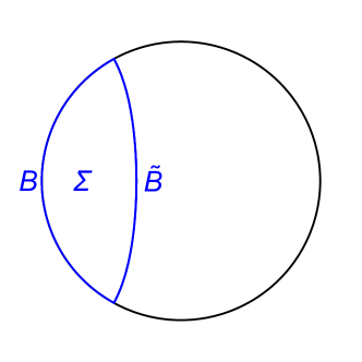
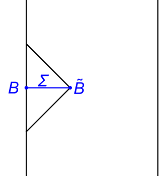
Figure 1: (Left) The $\tau=0$ slice of AdS. The region $B$ is on the boundary, $\tilde{B}$ is the bulk extremal surface, and $\Sigma$ is between them in the bulk. (Right) A cross-section of AdS, where time runs vertically. $\Sigma$ lies at $\tau=0$ and the causal wedge associated to $B$ is shown.

It so happens that, since we are considering such a simple surface in empty AdS, $\tilde{B}$ is also the boundary of the “causal wedge” associated to $B$. The causal wedge in the bulk is the set of all points whose past and future intersects the domain of dependence of $B$ on the boundary. We can cover the causal wedge with coordinates $t$, $\zeta$, and $u$ defined by

$$\cosh\zeta\sinh u =\tan\rho\sin\theta,$$ (9)

$$\sinh\zeta\sinh t =\frac{\sin\tau}{\cos\rho},$$ (10)

$$\cosh\zeta\cosh u+\cos\theta_{0}\sinh\zeta\cosh t =\sin\theta_{0}\frac{\cos\tau}{\cos\rho},$$ (11)

$$\cos\theta_{0}\cosh\zeta\cosh u+\sinh\zeta\cosh t =\sin\theta_{0}\tan\rho\cos\theta,$$ (12)

in terms of which the metric is of AdS-Rindler form:

$$ds^{2}=-\sinh^{2}\zeta dt^{2}+d\zeta^{2}+\cosh^{2}\zeta(du^{2}+\sinh^{2}ud\Omega_{d-2}^{2}).$$ (13)

We see that on the boundary, $\zeta\to\infty$, this choice of coordinates induces an $R\times H^{d-1}$ geometry on the domain of dependence of $B$. The surface $\tilde{B}$ is obtained by taking $\zeta\to 0$ at fixed $t$. The Killing vector $\xi^{a}=\partial_{t}$ generates time translations in this AdS-Rindler patch, and for calculations it is useful to have an expression for it in terms of the global coordinates:

$$\xi^{a}=\frac{\cos\tau\sin\rho\cos\theta-\cos\theta_{0}}{\sin\theta_{0}}\partial_{\tau}+\frac{\cos\theta\cos\rho\sin\tau}{\sin\theta_{0}}\partial_{\rho}-\frac{\sin\theta\sin\tau}{\sin\rho\sin\theta_{0}}\partial_{\theta}.$$ (14)

Notice that $\xi^{a}$ vanishes on $\tilde{B}$. We have normalized $\xi^{a}$ so that it has unit surface gravity, $\kappa=1$, where $\xi^{a}\nabla_{a}\xi^{b}=\kappa\xi^{b}$ on the Rindler horizon.

3 Holographic Entropy Calculation

The Area Term

First we will compute the area term. According to the Ryu-Takayanagi Ryu:2006bv prescription, we need to find the area of the extremal surface in the bulk which is anchored on the boundary of $B$. As is typically formulated, this term only makes sense when there is a well-defined notion of a classical geometry in the bulk. For our purposes a slight generalization is necessary. We will interpret the Ryu-Takayanagi term in the entropy to be the expectation value of the operator $\hat{A}$ which encodes the area of the extremal surface. This operator is a functional of the metric operator, which for small perturbations we can write as $g+\hat{h}$ with $g$ the AdS vacuum metric. In the low-temperature limit, we use (5) to write the difference between the finite-temperature area and the vacuum area as

$$\delta A(T)={\rm Tr}(\hat{A}\rho(T))-\left\langle 0\right|\hat{A}\left|0\right\rangle=e^{-\beta\Delta}\left(\left\langle\Delta\right|\hat{A}\left|\Delta\right\rangle-\left\langle 0\right|\hat{A}\left|0\right\rangle\right)+\cdots.$$ (15)

We are only interested in evaluating this difference to leading order in $G_{N}$, and so we can expand $\left\langle\Delta\right|\hat{A}\left|\Delta\right\rangle$ to first order in $\hat{h}$. Up to operator ordering ambiguities (which do not appear at linear order), $\hat{A}$ should equal $A[g+\hat{h}]$, where $A[\cdot]$ is just the classical functional of the metric which computes the area. Schematically, we have

$$\left\langle\Delta\right|\hat{A}\left|\Delta\right\rangle=\left\langle\Delta\right|A[g+\hat{h}]\left|\Delta\right\rangle=A[g]+\left.\frac{\delta A}{\delta h}\right|_{h=0}\left\langle\Delta\right|\hat{h}\left|\Delta\right\rangle+\cdots.$$ (16)

where $A[g]$ is the classical empty AdS value of the area, equal to $\left\langle 0\right|\hat{A}\left|0\right\rangle$ before quantum corrections. The result is that the first-order corrections to the quantum expectation value for the area can be computed by substituting the expectation value for the metric perturbation into the classical area functional, and expanding to first order. This is not the case for the higher-order corrections if the metric perturbation behaves non-classically, which is as we would expect from a single-particle state with a broad wavefunction like $\left|\Delta\right\rangle$.

Furthermore, to first order in $G_{N}$ the expectation value of the metric perturbation is obtained easily from the expectation value of the linearized Einstein equations:

$$E_{\mu\nu}[\langle\hat{h}\rangle]=\left\langle E_{\mu\nu}[\hat{h}]\right\rangle=8\pi G_{N}\left\langle\hat{T}^{\rm matter}_{\mu\nu}\right\rangle,$$ (17)

where we have introduced the notation $E_{\mu\nu}$ to denote the linearized equation of motion for the metric perturbation in the absence of matter (but including the cosmological constant). To summarize, at this order in perturbation theory we can obtain the correct backreaction of the matter on the geometry by treating $\langle\hat{T}^{\rm matter}_{\mu\nu}\rangle$ as a classical source. From now on we will simplify our notation by writing $\langle\hat{h}_{\mu\nu}\rangle=h_{\mu\nu}$ and $\langle\hat{T}^{\rm matter}_{\mu\nu}\rangle=T^{\rm matter}_{\mu\nu}$.

Now it is a simple matter to find $\delta A(T)$. The first-order correction to the extremal surface area is obtained by leaving the surface fixed and integrating the linear deviation of the area functional over that surface:

$$\delta A(T)=e^{-\beta\Delta}\int_{\tilde{B}}d^{d-1}x\,\left.\frac{\delta A}{\delta h_{\mu\nu}(x)}\right|_{h=0}h_{\mu\nu}(x).$$ (18)

Bulk Entropy

The calculation of the bulk entropy is similar to the CFT calculation in Ref. Herzog:2014fra . In the low-temperature limit, the reduced density operator for the region $\Sigma$ is found by taking the trace of (5) over the complement of $\Sigma$:

$$\rho_{\Sigma}(T)=\rho_{\Sigma}^{0}+e^{-\beta\Delta}(\rho_{\Sigma}^{\Delta}-\rho_{\Sigma}^{0})+\cdots$$ (19)

The second term is just a small perturbation, so we can apply the first law of entanglement entropy:

$$\delta S_{\rm bulk}(T)=-e^{-\beta\Delta}{\rm Tr}\left[\left(\rho_{\Sigma}^{\Delta}-\rho_{\Sigma}^{0}\right)\log\rho_{\Sigma}^{0}\right]=e^{-\beta\Delta}\delta K_{\Sigma},$$ (20)

where we have denoted by $\delta K_{\Sigma}$ the change in the expectation value of the vacuum modular Hamiltonian on $\Sigma$, $-\log\rho_{\Sigma}^{0}$. Recall that $\Sigma$ is a constant-time surface in the AdS-Rindler space constructed in Sec. 2. Much like flat Rindler space, the vacuum state of AdS-Rindler is obtained by a $2\pi$ tranlsation in Euclidean AdS-Rindler time. So the vacuum modular Hamiltonian in AdS-Rindler space is just $2\pi$ times time-translation Hamiltonian associated to that space, i.e., translation by $\xi^{a}$, which is the integral over $\Sigma$ of one of the components of the bulk stress tensor. Thus we have

$$\delta S_{\rm bulk}(T)=2\pi e^{-\beta\Delta}\int_{\Sigma}\xi^{\mu}T^{\rm matter}_{\mu\nu}d\Sigma^{\nu},$$ (21)

where $\xi^{a}=\partial_{t}$ is the AdS-Rindler Killing vector introduced previously, and $d\Sigma^{a}$ is the volume form on $\Sigma$.

Putting Things Together

Now we just have to put together (18) and (21) to get

$$\delta S^{\rm holo}_{B}(T) \equiv\frac{\delta A(T)}{4G_{N}}+\delta S_{\rm bulk}(T)$$ (22)

$$=e^{-\beta\Delta}\left[\frac{1}{4G_{N}}\int_{\tilde{B}}d^{d-1}x\frac{\delta A}{\delta h_{\mu\nu}(x)}h_{\mu\nu}(x)+2\pi\int_{\Sigma}\xi^{\mu}T^{\rm matter}_{\mu\nu}{\bf\epsilon}^{\nu}\right].$$ (23)

To see that this is equivalent to $\delta S^{\rm CFT}_{B}$ in (1), we make use of the $(d-1)$-form ${\bf\chi}$ constructed out of the metric perturbation $h$ in Ref. Faulkner:2013ica , which has the (off-shell) properties

$$\int_{\tilde{B}}{\bf\chi} =\frac{1}{4G_{N}}\int_{\tilde{B}}d^{d-1}x\left.\frac{\delta A}{\delta h_{\mu\nu}(x)}\right|_{h=0}h_{\mu\nu}(x),$$ (24)

$$\left.d{\bf\chi}\right|_{\Sigma} =-\frac{1}{4G_{N}}\xi^{\mu}E_{\mu\nu}[h]d\Sigma^{\nu}.$$ (25)

Additionally, the integral of $\chi$ over the surface $B$, which from the bulk point of view is the part of the boundary of $\Sigma$ located at infinity, can be written as

$$\int_{B}{\bf\chi}=\int_{B}d^{d-1}x\,\delta S_{B}^{\rm grav}[h],$$ (26)

where we still need to identify $\delta S_{B}^{\rm grav}[h]$. To do so, recall the holographic dictionary for the metric perturbation near the boundary (schematically):

$$\lim_{\rho\to\pi/2}\left(\frac{\pi}{2}-\rho\right)^{2-d}h_{\mu\nu}\sim\delta\left\langle T_{\mu\nu}^{\rm CFT}\right\rangle,$$ (27)

where $\delta\left\langle T_{\mu\nu}^{\rm CFT}\right\rangle$ is the vacuum-subtracted expectation value of the stress tensor in the CFT. The region $B$ is simple enough that $\delta K_{B}$, the vacuum-subtracted expectation value of the CFT vacuum modular Hamiltonian on $B$, can be written as a local integral of $\delta\left\langle T_{\mu\nu}^{\rm CFT}\right\rangle$:

$$\delta K_{B}\equiv-{\rm Tr}\left[\left(\rho_{B}-\rho_{B}^{0}\right)\log\rho_{B}^{0}\right]=\int_{B}\left(\text{local function of }\delta\left\langle T_{\mu\nu}^{\rm CFT}\right\rangle\right).$$ (28)

So, applying (27), $\delta K_{B}$ can be written as a local integral of the asymptotic value of the metric perturbation $h$ in the bulk. That local integral is precisely the right-hand side of (26), which defines $\delta S_{B}^{\rm grav}$. Said another way, the integral of $\chi$ over $B$ is $\delta K_{B}$ in the CFT translated into bulk language using the holographic dictionary (27).

If we evalutate (26) in the state $\left|\Delta\right\rangle$ we will find $\delta K_{B}$ in the state $\left|\Delta\right\rangle$. By including the Boltzmann factor, we obtain the first thermal correction to the CFT entanglement entropy of $B$ in a way entirely parallel with the bulk calculation in (20), and in fact this is how (1) was obtained by Herzog Herzog:2014fra . In other words, we have

$$e^{-\beta\Delta}\int_{B}{\bf\chi}=e^{-\beta\Delta}\int_{B}dx^{d-1}\delta S_{B}^{\rm grav}[h]=\delta S^{\rm CFT}_{B}(T),$$ (29)

where $\delta S^{\rm CFT}_{B}(T)$ is the quantity appearing in (1). We would like to emphasize that this follows directly from the definition of $\delta S_{B}^{\rm grav}$ and the property (26) of $\chi$.

Applying Stokes’ theorem to $\chi$ yields

$$-\int_{\Sigma}\frac{1}{4G_{N}}\xi^{\mu}E_{\mu\nu}[h]d\Sigma^{\nu}=\int_{\Sigma}d\chi=\int_{\tilde{B}}\chi-\int_{B}\chi=e^{\beta\Delta}\left[\frac{\delta A(T)}{4G_{N}}-\delta S^{\rm CFT}_{B}(T)\right]~{}.$$ (30)

The linearized Enstein equations, $E_{\mu\nu}=8\pi G_{N}T_{\mu\nu}^{\rm matter}$, then give

$$\delta S^{\rm CFT}_{B}(T)=\frac{\delta A(T)}{4G_{N}}+2\pi e^{-\beta\Delta}\int_{\Sigma}\xi^{\mu}T_{\mu\nu}^{\rm matter}d\Sigma^{\nu}=\frac{\delta A(T)}{4G_{N}}+\delta S_{\rm bulk}(T)=\delta S^{\rm holo}_{B}(T),$$ (31)

completing the argument. Note that this guarantees that $\delta S^{\rm CFT}_{B}=\delta S^{\rm holo}_{B}$ even without knowing the explicit form of $\delta S^{\rm CFT}_{B}(T)$. As an illustration, we go through an example in Appendix A where the exact expression in (1) is reproduced directly from the bulk.

4 Discussion

We have shown that the first thermal corrections to CFT entanglement entropy can be produced from a purely bulk calculation. There are two main ideas that came together to accomplish this. First, as was already noticed in Refs. Faulkner:2013ica ; Swingle:2014uza , there is a deep connection between the linearized Einstein equations in the bulk, the modular Hamiltonian on the boundary, and the linearized area functional on the extremal surface. The context here is a little different, though. In Refs. Faulkner:2013ica ; Swingle:2014uza , the bulk geometry was assumed classical, and the differential form $\chi$ was used to derive the linearized Einstein equations for that classical metric from the properties of entanglement entropy on the boundary. Here we are assuming the Einstein equations, in the form of operator equations inside of expectaion values, and using them to learn something about the entanglement entropy. The differential form $\chi$ connects the bulk and the boundary in the same way, but the direction of the argument has switched around.

The second main idea was in our treatment of the Ryu-Takayanagi area functional. The metric backreaction was not assumed classical, but still gave a contribution to the area of the extremal surface. The idea that the Ryu-Takayanagi term should be thought of as an expectation value is very natural, but is difficult to test in a nontrivial way. Here we really only used the mild assumption that it behaves as an expectation value with respect to thermal averaging and linear quantum corrections. For higher-order corrections, it would be important to treat this term in the correct way (which likely involves using the generalized entropy in the bulk instead of the area and bulk entanglement separately Engelhardt:2014gca ). It would be very interesting if a more nontrivial example could be found, such as one where off-diagonal matrix elements of $\hat{A}$ were important.

Appendix A Example: Bulk Scalar Field

In this appendix we will work through an example where the lowest-energy state is that of a free scalar field in the bulk, of mass $m^{2}=\Delta(\Delta-d)$. The lowest energy state is the one with zero angular momentum and zero radial quantum number. Let $a^{\dagger}$, $a$ be the creation and annihilation operators for this state, in terms of which the field can be written as

$$\phi=N(ae^{i\Delta\tau}+a^{\dagger}e^{-i\Delta\tau})\cos^{\Delta}\rho+\cdots,$$ (32)

where $N$ is a normalization constant to be fixed later and the $\cdots$ represent creation/annihilation operators for other modes which do not concern us. In the state $\left|\Delta\right\rangle=a^{\dagger}\left|0\right\rangle$, the the expectation value of the energy-momentum tensor is spherically symmetric and time-independent, and in particular the energy density is

$$T^{\rm matter}_{\tau\tau}=N^{2}\Delta\left(\Delta-\frac{d}{2}\right)\cos^{2\Delta-2}\rho.$$ (33)

The coefficient $N^{2}$ can be computed by demanding that the total energy is equal to $\Delta$. In fact, all we need to know about the energy-momentum tensor is that it is time-independent, spherically symmetric, and that the total energy is $\Delta$. Because of the symmetries, the perturbed metric looks like a black hole with a radially-varying mass. It is most convenient to add the perturbation to the global metric using the coordinate $r=\tan\rho$, in which case we have to first order

$$ds^{2}=-\left(1+r^{2}-\frac{\mu(r)}{r^{d-2}}\right)d\tau^{2}+\frac{1}{1+r^{2}}\left(1+\frac{\mu(r)}{(1+r^{2})r^{d-2}}\right)dr^{2}+r^{2}d\Omega_{d-1}^{2},$$ (34)

with

$$\mu(r)=\frac{16\pi G_{N}}{d-1}\int_{0}^{r}dr^{\prime}\frac{r^{\prime d-1}}{1+r^{\prime 2}}\,T^{\rm matter}_{\tau\tau}(r^{\prime}).$$ (35)

It’s straightforward to check that the deviation in the area of $\tilde{B}$ due to this metric perturbation is

$$\delta A(T)=\frac{e^{-\beta\Delta}\Omega_{d-2}}{2}\int_{0}^{\theta_{0}}d\theta~{}\sin^{d-2}\theta\frac{\tan^{2}\theta}{\tan\theta_{0}}\mu(\rho(\theta)),$$ (36)

where we use $\sin\rho\cos\theta=\cos\theta_{0}$ for the surface $\tilde{B}$. By substituting the expression (14) for $\xi^{a}$ into equation (21) for the bulk entropy we find

$$\delta S_{\rm bulk}(T)=2\pi\Omega_{d-2}e^{-\beta\Delta}\int_{\Sigma}d\rho d\theta\sin^{d-2}\theta\tan^{d-1}\rho\frac{\sin\rho\cos\theta-\cos\theta_{0}}{\sin\theta_{0}}\,T^{\rm matter}_{\tau\tau}(\rho).$$ (37)

We know from the general discussion of the text that we should make use of Einstein’s equation to find an expression for $\mu$ in terms of $T^{\rm matter}_{\tau\tau}$. In this case, the $\tau\tau$-component of Einstein’s equation says

$$T^{\rm matter}_{\tau\tau}(r)=\frac{d-1}{16\pi G_{N}}\frac{1+r^{2}}{r^{d-1}}\frac{d\mu}{dr},$$ (38)

as is evident from (35). Substituting this in for $T^{\rm matter}_{\tau\tau}$ gives

$$\delta S_{\rm bulk}(T)=\frac{d-1}{8G_{N}}\Omega_{d-2}e^{-\beta\Delta}\int_{\Sigma}d\rho d\theta\sin^{d-2}\theta\frac{\sin\rho\cos\theta-\cos\theta_{0}}{\sin\theta_{0}}\frac{d\mu}{d\rho}.$$ (39)

Being clever, we can choose to rewrite the integrand as

$$\sin^{d-2}\theta\frac{\sin\rho\cos\theta-\cos\theta_{0}}{\sin\theta_{0}}\frac{d\mu}{d\rho}=\partial_{\rho}\chi^{\theta}-\partial_{\theta}\chi^{\rho},$$ (40)

with

$$\chi^{\rho} =\frac{1}{d-1}\frac{\cos\rho\sin^{d-1}\theta}{\sin\theta_{0}}\mu(\rho),$$ (41)

$$\chi^{\theta} =\frac{\sin\rho\cos\theta-\cos\theta_{0}}{\sin\theta_{0}}\mu(\rho)\sin^{d-2}\theta.$$ (42)

This allows us to use Green’s theorem:

$$\delta S_{\rm bulk}(T)=\frac{d-1}{8G_{N}}\Omega_{d-2}e^{-\beta\Delta}\left[\int_{0}^{\theta_{0}}d\theta\,\left.\chi^{\theta}\right|_{\rho=\pi/2}-\int_{0}^{\theta_{0}}d\theta\,\left.\left(\chi^{\theta}+\frac{d\rho}{d\theta}\chi^{\rho}\right)\right|_{\sin\rho=\cos\theta_{0}/\cos\theta}\right].$$ (43)

The first term reproduces the function in (1),

$$\frac{d-1}{8G_{N}}\Omega_{d-2}e^{-\beta\Delta}\int_{0}^{\theta_{0}}d\theta\,\left.\chi^{\theta}\right|_{\rho=\pi/2}=\Delta e^{-\beta\Delta}I_{d}(\theta_{0}),$$ (44)

while the second term gives us the change in area,

$$\frac{d-1}{8G_{N}}\Omega_{d-2}e^{-\beta\Delta}\int_{0}^{\theta_{0}}d\theta\,\left.\left(\chi^{\theta}+\frac{d\rho}{d\theta}\chi^{\rho}\right)\right|_{\sin\rho=\cos\theta_{0}/\cos\theta}=\frac{\delta A(T)}{4G_{N}}.$$ (45)

So we have successfully derived (1) from a bulk calculation.

References

- (1) C. P. Herzog, “Universal Thermal Corrections to Entanglement Entropy for Conformal Field Theories on Spheres,” JHEP 1410 (2014) 28, arXiv:1407.1358 [hep-th].
- (2) H. Casini, F. Mazzitelli, and E. T. Lino, “Area terms in entanglement entropy,” arXiv:1412.6522 [hep-th].
- (3) S. Ryu and T. Takayanagi, “Holographic derivation of entanglement entropy from AdS/CFT,” Phys.Rev.Lett. 96 (2006) 181602, arXiv:hep-th/0603001 [hep-th].
- (4) T. Faulkner, A. Lewkowycz, and J. Maldacena, “Quantum corrections to holographic entanglement entropy,” JHEP 1311 (2013) 074, arXiv:1307.2892.
- (5) T. Faulkner, M. Guica, T. Hartman, R. C. Myers, and M. Van Raamsdonk, “Gravitation from Entanglement in Holographic CFTs,” JHEP 1403 (2014) 051, arXiv:1312.7856 [hep-th].
- (6) V. Iyer and R. M. Wald, “Some properties of Noether charge and a proposal for dynamical black hole entropy,” Phys.Rev. D50 (1994) 846–864, arXiv:gr-qc/9403028 [gr-qc].
- (7) B. Swingle and M. Van Raamsdonk, “Universality of Gravity from Entanglement,” arXiv:1405.2933 [hep-th].
- (8) N. Engelhardt and A. C. Wall, “Quantum Extremal Surfaces: Holographic Entanglement Entropy beyond the Classical Regime,” JHEP 1501 (2015) 073, arXiv:1408.3203 [hep-th].