Entropy of finite random binary sequences with weak long-range correlations

Abstract

We study the $N$-step binary stationary ergodic Markov chain and analyze its differential entropy. Supposing that the correlations are weak we express the conditional probability function of the chain through the pair correlation function and represent the entropy as a functional of the pair correlator. Since the model uses the two-point correlators instead of the block probability, it makes it possible to calculate the entropy of strings at much longer distances than using standard methods. A fluctuation contribution to the entropy due to finiteness of random chains is examined. This contribution can be of the same order as its regular part even at the relatively short lengths of subsequences. A self-similar structure of entropy with respect to the decimation transformations is revealed for some specific forms of the pair correlation function. Application of the theory to the DNA sequence of the R3 chromosome of Drosophila melanogaster is presented.

I Introduction

At present there is a commonly accepted viewpoint that our world is complex and correlated. The most peculiar manifestations of this concept are the records of brain activity and heart beats, human and animal communication, written texts of natural languages, DNA and protein sequences, data flows in computer networks, stock indexes, sun activity, weather (the chaotic nature of the atmosphere), etc. For this reason systems with long-range interactions (and/or with long-range memory) and natural sequences with non-trivial information content have been the focus of a large number of studies in different fields of science over the past several decades.

Random sequences with finite number of states exist as natural sequences (DNA or natural texts) or arise as a result of coarse-grained mapping of the evolution of the chaotic dynamic system into a string of symbols Eren ; Lind . Such sequences are very closely connected to and are the subject of study of the algorithmic (Kolmogorov-Solomonoff-Chaitin) complexity, artificial intellect, information theory, compressibility of digital data, statistical inference problem, computability Cover and have many application aspects as a creative tool for designing the devices and appliances with random components in their structure IzrKrMak (different wave-filters, diffraction gratings, artificial materials, antennas, converters, delay lines, etc.).

There are many methods for describing complex dynamical systems and random sequences connected with them: correlation function, fractal dimensions, multi-point probability distribution functions, and many others. One of the most convenient characteristics serving to the purpose of studying complex dynamics is entropy Shan ; Cover . Being a measure of the information content and redundancy in a sequence of data, it is a powerful and popular tool in examination of complexity phenomena. It has been used for the analysis of a number of different dynamical systems.

A standard method of understanding and describing statistical properties of real physical systems or random sequences of data can be represented as follows. First of all, we have to analyze the sequence to find the correlation functions or the probabilities of words occurring, with the length $L$ exceeding the correlation length $R_{c}$ but being shorter than the length $M$ of the sequence,

$$R_{c}<L\ll M.$$ (1)

At the same time, the number $d^{L}$ of different words of the length $L$ composed in the alphabet containing $d$ letters has to be much less than the number $M-L$ of words in the sequence,

$$d^{L}\ll M-L\approx M.$$ (2)

The next step is to express the correlation properties of the sequence in terms of the conditional probability function (CPF) of the Markov chain, see below Eq. (5). Note, the Markov chain should be of order $N$, which is supposed to be longer than the correlation length,

$$R_{c}<N.$$ (3)

This is the critical requirement because the correlation length of natural sequence of interest (e.g., written or DNA texts) is usually of the same order as the length of sequences. None of inequalities $(\ref{Strong})-(\ref{Strong3})$ can be fulfilled. Really, the lengths of words that could represent correctly the probability of words occurring are $4-5$ letters for a real natural text of the length $10^{6}$ (written on an alphabet containing $27-30$ letters and symbols) or of order of 20 symbols for a coarse-grained text represented by means of a binary sequence.

Here we develop an approach that is complimentary to the above exposed. In particular, we represent the conditional probability function of the Markov chain by means of pair correlator, which makes it possible to calculate analytically the entropy of the sequence. It should be stressed that the standard method for calculating the entropy can only take into account the short-range part of statistics. We present a theory that expresses long-range correlation properties through the correlation functions.

The scope of the paper is as follows. First, we discuss briefly the properties of the $N$-step additive Markov chain model and, supposing that the correlations between symbols in the sequence are weak, we express the conditional probability function by means of the pair correlation function. In the next section we represent the differential entropy in terms of the conditional probability function of the Markov chain and express the entropy as the sum of squares of the pair correlators. Then we discuss some properties of the results obtained, in particular, a property of self-similarity of entropy with respect to decimation for some particular classes of the Markov chains. Next, a fluctuation contribution to the entropy due to finiteness of random chains is examined. Some remarks on literary texts are followed by discussions of directions in which the research can be progressed.

II Additive Markov chains

This section includes mainly introductory material. Some authors’ results presented by Eqs. (II)–(14) were exposed earlier in Ref. muya ; RewUAMM ; MUYaG ; highord ; UYa .

Consider a semi-infinite sequence $\mathbb{A}=a_{0}^{\infty}=a_{0},a_{1},a_{2},...$ of real random variables $a_{i}$ taken from the finite alphabet $A=\{1,2,...,d\}$, $a_{i}\in A$. The sequence $\mathbb{A}$ is an $N$-step Markov chain if it possesses the following property: the probability of symbol $a_{i}$ to have a certain value $a$ under the condition that the values of all other symbols are given depends only on the values of $N$ previous symbols,

$$P(a_{i}=a|\ldots,a_{i-2},a_{i-1})$$

$$=P(a_{i}=a|a_{i-N},\ldots,a_{i-2},a_{i-1}).$$ (4)

Note, definition (II) is valid for $i\geq N$; for $i<N$ we have to use the well known conditions of compatibility for the conditional probability functions of the lower order, Ref. shir . Sometimes the number $N$ is also referred to as the order or the memory length of the Markov chain. The conditional probability function (CPF) $P(a_{i}=a|a_{i-N},\ldots,a_{i-2},a_{i-1})$ determines completely all statistical properties of the Markov chain and the method of their iterative numerical construction. If the sequence, statistical properties of which we would like to analyze is assigned, the conditional probability function of the $N$-th order can be found by a standard method,

$$P(a_{N+1}=a|a_{1},\ldots,a_{N})=\frac{P(a_{1},\ldots,a_{N},a)}{P(a_{1},\ldots,a_{N})},$$ (5)

where $P(a_{1},\ldots,a_{N})$ is the probability of the $N$-words $a_{1},\ldots,a_{N}$ occurring.

The Markov chain determined by Eq. (II) is a homogeneous sequence because its conditional probability does not depend explicitly on $i$, i.e., is independent of the position of symbols $a_{i-N},\ldots,a_{i-1},a_{i}$ in the chain. It depends only on the values of symbols $a_{i-N},\ldots,a_{i-1},a_{i}$. The homogeneous sequences are stationary: the average value of any function $f(a_{r_{1}},a_{r_{1}+r_{2}},\ldots,a_{r_{1}+\ldots+r_{s}})$ of $s$ arguments

$$\overline{f}\,(a_{r_{1}},\ldots,a_{r_{1}+\ldots+r_{s}})$$ (6)

$$=\lim_{M\to\infty}\frac{1}{M}\sum_{i=0}^{M-1}f(a_{i+r_{1}},\ldots,a_{i+r_{1}+\ldots+r_{s}})$$

depends on $s-1$ differences between the indexes. In other words, all statistically averaged functions of random variables are shift-invariant.

We suppose that the chain is ergodic. According to the Markov theorem (see, e.g., Ref. shir ), this property is valid for the homogenous Markov chains if the strict inequalities,

$$0<P(a_{i+N}=\alpha|a_{i}^{i+N-1})<1,\,i\in\mathbb{N}_{+}=\{0,1,...\}$$ (7)

are fulfilled for all possible values of the arguments in function (II). Hereafter we use the shorter notation $a_{i-N}^{i-1}$ for $N$-word $a_{i-N},...,a_{i-1}$. It follows from ergodicity that the correlations between any blocks of symbols in the chain go to zero when the distance between them goes to infinity. The other consequence of ergodicity is the possibility to use one random sequence as an equitable representative of the ensemble of chains and to do averaging over the sequence, Eq. (6), instead of an ensemble averaging.

Below we will consider an important class of the binary random sequences with symbols $a_{i}$ taking on two values, say $0$ and $1$, $a_{i}\in\{0,1\}$. The conditional probability to find $i$-th element $a_{i}=1$ in the binary $N$-step Markov sequence depending on $N$ preceding elements $a_{i-N}^{i-1}$ is a set of $2^{N}$ numbers:

$$P(1|a_{i-N}^{i-1})=P(a_{i}=1|a_{i-N}^{i-1}),$$

$$P(0|a_{i-N}^{i-1})=1-P(1|a_{i-N}^{i-1}).$$ (8)

Conditional probability (II) of the binary sequence of random variables $a_{i}\in\{0,1\}$ can be represented exactly as a finite polynomial series:

$$P(1|a_{i-N}^{i-1})=\bar{a}+\sum_{r_{1}=1}^{N}F_{1}(r_{1})(a_{i-r_{1}}-\bar{a})$$

$$+\sum_{r_{1},r_{2}=1}^{N}F_{2}(r_{1},r_{2})(a_{i-r_{1}}a_{i-r_{2}}-\overline{a_{i-r_{1}}a_{i-r_{2}}})+\ldots$$

$$+\sum_{r_{1},\ldots,r_{N}=1}^{N}F_{N}(r_{1},\ldots,r_{N})(a_{i-r_{1}}\ldots a_{i-r_{N}}$$

$$-\,\,\overline{a_{i-r_{1}}\ldots a_{i-r_{N}}}),$$ (9)

where the statistical averages $\overline{a_{r_{1}}\ldots a_{r_{N}}}$ are taken over sequence (6), $F_{s}$ is the family of memory functions and $\bar{a}$ is the relative average number of unities in the sequence. The representation of Eq. (II) in the form of Eq. (II) follows from the simple identical equalities, $a^{2}=a$ and $f(a)=af(1)+(1-a)f(0)$, for an arbitrary function $f(a)$ determined on the set $a\in\{0,1\}$. The first term in Eq. (II) is responsible for generation of uncorrelated white-noise sequences. Taking into account the second term, proportional to $F_{1}(r)$, we can reproduce correctly correlation properties of the chain up to the second order. Higher-order correlators and all correlation properties of higher orders are not independent anymore. We cannot control them and reproduce correctly by means of the memory function $F(r)$, because the latter is completely determined by the pair correlation function, see below Eq. (11). Studying of the properties of these higher-order correlators is beyond the scope of this paper. In what follows we will only use the first two terms, which determine the so-called additive Markov chain muya ; RewUAMM .

A particular form of the conditional probability function of additive Markov chain is the chain with step-wise memory function,

$$P(1|k)=\frac{1}{2}+\mu\left(\frac{2k}{N}-1\right).$$ (10)

The probability $P(1|k)$ of having the symbol $a_{i}=1$ after $N$-word $a_{i-N}^{i-1}$ containing $k$ unities, $\,\,k=\sum_{l=1}^{N}a_{i-l}$, is a linear function of $k$ and is independent of the arrangement of symbols in the word $a_{i-N}^{i-1}$. The parameter $\mu$ characterizes the strength of correlations in the system.

There is a rather simple relation between the memory function $F(r)$ (hereafter we will omit the subscript $1$ of $F_{1}(r)$) and the pair correlation function of the binary additive Markov chain. There were suggested two methods for finding the $F(r)$ of a sequence with a known pair correlation function. The first one muya is based on the minimization of a “distance”  between the Markov chain generated by means of the sought-for memory function and the initial given sequence of symbols with a known correlation function. The minimization equation yields the relationship between the correlation and memory functions,

$$K(r)=\sum\limits_{r^{\prime}=1}^{N}F(r^{\prime})K(r-r^{\prime}),\ \ \ \ r\geqslant 1.$$ (11)

where the normalized correlation function $K(r)$ is given by

$$K(r)=\frac{C(r)}{C(0)},\quad C(r)=\overline{(a_{i}-\bar{a})(a_{i+r}-\bar{a})}.$$ (12)

The second method for deriving Eq. (11) is the completely probabilistic straightforward calculation MUYaG .

Equation (11), despite its simplicity, can be analytically solved only in some particular cases: for one- or two-step chains, Markov chain with step-wise memory function and so on. To avoid the difficulties in solving Eq. (11) we suppose that correlations in the sequence are weak. This means that all components of the normalized correlation function are small, $|K(r)|\ll 1,\,|r|\neq 0$, with the exception of $K(0)=1$. So, taking into account that in the sum of Eq. (11) the leading term is $K(0)=1$ and all the others are small, we can obtain an approximate solution for the memory function in the form of the series

$$F(r) = K(r)-\sum_{r^{\prime}\neq r}^{N}K(r-r^{\prime})K(r^{\prime})$$

$$+ \sum_{r^{\prime}\neq r}^{N}\sum_{r^{\prime\prime}\neq r^{\prime}}^{N}K(r-r^{\prime})K(r^{\prime}-r^{\prime\prime})K(r^{\prime\prime})+...$$

The equation for the conditional probability function in the first approximation with respect to the small functions $|K(r)|\ll 1,\,|r|\neq 0$ takes the form

$$P(1|a_{i-N}^{i-1}) \simeq \bar{a}+\sum_{r=1}^{N}F(r)(a_{i-r}-\bar{a})$$ (14)

$$\simeq \bar{a}+\sum_{r=1}^{N}K(r)(a_{i-r}-\bar{a}).$$

This formula provides a very important tool for constructing a sequence with a given pair correlation function. Note that $i$-independence of the function $P(1|a_{i-N}^{i-1})$ guarantees homogeneity and stationarity of the sequence under consideration; and finiteness of $N$ provides its ergodicity. Evidently, we can only consider sequences with the correlation functions, determined by $P(1|a_{i-N}^{i-1})$, which satisfy Eq. (7).

The correlation functions are typically employed as the input characteristics for describing the random sequences. However, the correlation function describes not only the direct interconnection of the elements $a_{i}$ and $a_{i+r}$, but also takes into account their indirect interaction via all other intermediate elements. Our approach operates with the “origin” characteristics of the system, specifically, with the memory function. The correlation and memory functions are mutually complementary characteristics of a random sequence in the following sense. The numerical analysis of a given random sequence enables one to determine directly the correlation function rather than the memory function. On the other hand, it is possible to construct a random sequence using the memory function, but not the correlation one, in the general case. Therefore, the memory function permits one to get a deeper insight into the intrinsic properties of the correlated systems. Equation (14) shows that in the limit of weak correlations both functions play the same role.

The concept of the additive Markov chain was extensively used earlier for studying random sequences with long-range correlations. The examples and references can be found in Ref. RewUAMM .

III Differential entropy

In order to estimate the entropy of an infinite stationary sequence $\mathbb{A}$ of symbols $a_{i}$ one could use the block entropy,

$$H_{L}=-\sum_{a_{1},...,a_{L}}P(a_{1}^{L})\log_{2}P(a_{1}^{L}).$$ (15)

Here $P(a_{1}^{L})=P(a_{1},\ldots,a_{L})$ is the probability to find the $L$-word $a_{1}^{L}$ in the sequence. The differential entropy, or entropy per symbol, is given by

$$h_{L}=H_{L+1}-H_{L},$$ (16)

and specifies the degree of uncertainty of the $(L+1)$th symbols observing if the preceding $L$ symbols are known. The source entropy (or Shannon entropy) is the differential entropy at the asymptotic limit, $h=\lim_{L\rightarrow\infty}h_{L}$. This quantity measures the average information per symbol if all correlations, in the statistical sense, are taken into account.

The differential entropy $h_{L}$ can be presented in terms of the conditional probability function. To show this we have to rewrite Eq. (15) for the block of length $L+1$, express $P(a_{1}^{L+1})$ via the conditional probability, and after a bit of algebra we obtain

$$h_{L}=\!\!\!\sum_{a_{1},...,a_{L}=0,1}\!\!\!P(a_{1}^{L})h(a_{L+1}|a_{1}^{L})=\overline{h(a_{L+1}|a_{1}^{L})}.$$ (17)

Here $h(a_{L+1}|a_{1}^{L})$ is the amount of information contained in the $(L+1)$-th symbol of the sequence conditioned on $L$ previous symbols,

$$h(a_{L+1}|a_{1}^{L})=-\!\!\!\sum_{a_{L+1}=0,1}\!\!\!P(a_{L+1}|a_{1}^{L})\log_{2}P(a_{L+1}|a_{1}^{L}).$$ (18)

So, the differential entropy $h_{L}$ of random sequence is presented as a special case of the standard conditional entropy $H=-\sum_{C}P(C)\sum_{B}P(B|C)\log_{2}P(B|C)$.

The conditional probability $P(1|a_{i-L}^{i-1})$ at $L<N$,

$$P(1|a_{i-L}^{i-1})\simeq\bar{a}+\delta;\quad\delta=\sum_{r=1}^{L}F(r)(a_{i-r}-\bar{a}),$$ (19)

is obtained in the first approximation in the parameter $\delta$ from Eq. (14) by means of the probabilistic reasoning presented in the Appendix.

Taking into account the weakness of correlations, $|\delta|\ll\min[\overline{a},(1-\overline{a})]$, one can expand the right-hand side of Eq. (18) in Taylor series up to the second order in $\delta$, $h(a_{L+1}|a_{1}^{L})=h_{0}+(\partial h/\partial\overline{a})_{|\delta=0}\delta+(1/2)(\partial^{2}h/\partial\overline{a}^{2})_{|\delta=0}\delta^{2}$, where the derivatives are taken at the “equilibrium point” $P(1|a_{i-L}^{i-1})=\bar{a}$ and $h_{0}$ is the entropy of uncorrelated sequence,

$$h_{0}=-\bar{a}\log_{2}(\bar{a})-(1-\bar{a})\log_{2}(1-\bar{a}).$$ (20)

Upon using Eq. (17) for averaging $h(a_{L+1}|a_{1}^{L})$ and in view of $\overline{\delta}=0$, the differential entropy of the sequence becomes

$$h_{L}=\left\{\begin{array}[]{l}h_{L\leq N}=h_{0}-\dfrac{1}{2\ln 2}\sum_{r=1}^{L}F^{2}(r),\\ h_{L>N}=h_{L=N}.\end{array}\right.$$ (21)

If the length of block exceeds the memory length, $L>N$, the conditional probability $P(1|a_{i-L}^{i-1})$ depends only on $N$ previous symbols, see Eq. (II). Then, it is easy to show from (17) that the differential entropy remains constant at $L\geq N$. The second line of Eq. (21) is consistent with the first one because in the first approximation in $\delta$ the correlation function vanishes at $L>N$ together with the memory function. The final expression, the main result of the paper, for the differential entropy of the stationary ergodic binary weakly correlated random sequence is

$$h_{L}=h_{0}-\frac{1}{2\ln 2}\sum_{r=1}^{L}K^{2}(r).$$ (22)

IV Discussion

It follows from Eq. (22) that the additional correction to the entropy $h_{0}$ of the uncorrelated sequence is the negative and monotonously decreasing function of $L$. This is the anticipated result — the correlations decrease the entropy. The conclusion is not sensitive to the sign of correlations: persistent correlations, $K>0$, describing an “attraction” of the symbols of the same kind, and anti-persistent correlations, $K<0$, corresponding to an attraction between “0” and “1”, provide the corrections of the same negative sign. If the correlation function is constant at $1\leqslant r\leqslant N$, the entropy is a linear decreasing function of the argument $L$ up to the point $N$; the result is coincident with that obtained in Ref. DMBUYa (in the limit of weak correlations) for the Markov chain model with step-wise memory function (10).

As an illustration of result (22), in Fig. 1 we present the plot of the differential entropy versus the length $L$. Both numerical and analytical results (the dotted and solid curves) are presented for the power-law correlation function $K(r)=0.01/r^{1.1}$. The cut–off parameter $r_{c}$ of the power-law function for numerical generation of the sequence, coinciding with the memory length of the chain, is $10^{4}$. The good agreement between the curves is the manifestation of adequateness of the additive Markov chain approach for studying entropy properties of random chains. The abrupt deviation of the dashed line from the upper analytical and numerical curves at $L\sim 10$ is the result of violation of inequality (2) and a manifestation of quickly growing errors in the entropy estimation by using the probability $P(a_{1},\ldots,a_{L})$ of the $L$ blocks occurring. Note that violation of Eq.(2) does not depend on the choice of the model parameter. It only depends on the length $M$ of the random sequence.

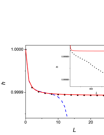
Figure 1: The differential entropy vs the length of words. The solid line is the analytical result, Eq. (22), for the correlation function $K(r)=0.01/r^{1.1}$ and $\bar{a}=1/2$, whereas the dots correspond to the direct evaluations of the same Eq. (22) for the numerically constructed sequence (of the length $M=10^{8}$ and the cut-off parameter $r_{c}=10^{4}$) by means of conditional probability function (14) and the numerically evaluated correlation function $K(r)$ of the constructed sequence. The dashed line is the differential entropy, Eqs. (15) and (16), plotted by using the numerical estimation of probability $P(a_{1},\ldots,a_{L})$ of the $L$-blocks occurring in the same sequence. The inset demonstrate the linear dependence of differential entropy at large $L$ governed by fluctuations of the correlation function.

In the main panel of Fig. 1 the deviation of numerical curve from analytical one is nearly absent. Nevertheless in the large scale, presented in the inset, a systematic linear deviation of numerical result from the analytical one is clearly seen. Explication of this phenomenon is given in the next section while discussing finite random sequences.

Our next illustration of applicability of the developed theory deals with the DNA sequence of the R3 chromosome of Drosophila melanogaster. In Fig. 2 the plot of the differential entropy versus the length $L$ is presented. We see that coincidence of the two approaches only holds for $L\lesssim 5-6$ units. It is difficult to do a single-valued conclusion of which factor, finiteness of the chain and violation of Eq. (2) or strength of correlations, is more important for discrepancy between two theories. Nevertheless, even observed coincidence between two curves seems rather astonishing.

Markov’s chains with step-wise memory functions and a larger class of permutable chains are invariant under decimation procedure UYa . Chains whose conditional probability functions are independent of the order of symbols in the $N$ word preceding a generated symbol are referred to as permutable. The decimation is a reduction of a random sequence by regular or random removing some part of symbols from the whole chain. It was shown in Refs. UYa ; highord that after decimation the correlation function of indicated classes of sequences is invariant up to the new reduced memory length $N^{*}=\lambda N$, where $\lambda$ is the relative non removed part of symbols in the chain. Hence, after decimation Eq. (21) does not change its form, but instead of $N$ we have only to put the new memory length $N^{*}$.

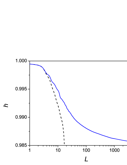
Figure 2: Differential entropy $h$ vs length $L$ for R3 chromosome of Drosophila melanogaster DNA of length $M\simeq 2.7\times 10^{7}$. The solid line is obtained by using Eq. (22) with numerically evaluated correlation function Eq. (12). The dashed line is the differential entropy, Eqs. (15) and (16), plotted by using the numerical estimation of probability $P(a_{1},\ldots,a_{L})$ of the $L$ blocks occurring in the same sequence.

V Finite random sequences

The relative average number of unities $\bar{a}$, correlation functions and other statistical characteristics of random sequences are deterministic quantities only in the limit of their infinite lengths. It is the direct consequence of the law of large numbers. If the length $M$ of the sequence is finite, the set of numbers $a_{1}^{M}$ cannot be considered anymore as ergodic sequence. In order to restore its status we have to introduce an ensemble of finite sequences $\{a_{1}^{M}\}_{p},p\in\mathbb{N}=0,1,2,...$. However, we would like to retain the right to examine finite sequences even if approximately by using a single finite chain. So, for a finite chain we have to replace definition (12) of the correlation function by the following one,

$$C_{M}(r)=\frac{1}{M-r}\sum_{i=0}^{M-r-1}(a_{i}-\bar{a})(a_{i+r}-\bar{a}),$$ (23)

$$\bar{a}=\frac{1}{M}\sum_{i=0}^{M-1}a_{i}.$$

Now the correlation functions and $\bar{a}$ are random quantities depending on a particular realization of the sequence $a_{1}^{M}$. Their fluctuations can contribute to the entropy of finite random chains even if the correlations in the random sequence are absent. It is well known that the order of relative fluctuations of additive random quantity (as, e.g. the correlation function Eq. (23)) is $1/\sqrt{M}$.

Below we give more rigorous justification of this explanation and show its applicability to our case. Let us present the correlation function $C_{M}(r)$ as the sum of two components,

$$C_{M}(r)=C(r)+C_{f}(r),$$ (24)

where the first summand $C(r)=\lim_{M\rightarrow\infty}C_{M}(r)$ is the correlation function determined by Eqs. (12) and (23), obtained by averaging over the sequence with respect to the index $i$, numbering the elements $a_{i}$ of the sequence $\mathbb{A}$; and the second one, $C_{f}(r)$, is a fluctuation–dependent contribution. The function $C(r)$ can be also presented as the ensemble average $C(r)=\langle C_{M}(r)\rangle$ due to ergodicity of the sequence.

Now we can find a connection between variances of $C_{M}(r)$ and $C_{f}(r)$. Taking into account that the correlations are weak and neglecting their contribution into $C_{f}(r)$ we have

$$\langle C^{2}_{M}(r)\rangle=C^{2}(r)+\langle C^{2}_{f}(r)\rangle.$$ (25)

In order to obtain the last equation we used Eq. (24) and the property of the function $\langle C_{f}(r)\rangle=0$ at $r\neq 0$. The mean fluctuation of the squared correlation function $C^{2}_{f}(r)$ is

$$\langle C^{2}_{f}(r)\rangle=\frac{1}{(M-r)^{2}}\sum_{n,m=0}^{M-r-1}\langle(a_{n}-\bar{a})(a_{n+r}-\bar{a})$$

$$\times(a_{m}-\bar{a})(a_{m+r}-\bar{a})\rangle.$$ (26)

Neglecting correlations between the elements $a_{n}$ and taking into account that only the terms with $n=m$ give nonzero contribution into the result we easily obtain

$$\langle K^{2}_{f}(r)\rangle=\frac{\langle C^{2}_{f}(r)\rangle}{C^{2}_{f}(0)},\,\,\langle K^{2}_{f}(r)\rangle=\frac{1}{M-r}\simeq\frac{1}{M}.$$ (27)

Note that Eq. (27) is obtained by means of averaging over the ensemble of chains. This is the shortest way to obtain the desired result. At the same time, for numerical simulations we used only averaging over the chain as is seen from Eq. (23), where summation over the sites $i$ of the chain plays the role of averaging.

Note also that different symbols $a_{i}$ in Eq. (V) are correlated. It is possible to show that contribution of their correlations to $\langle K^{2}_{f}(r)\rangle$ is of order $R_{c}/M^{2}\ll 1/M$.

The fluctuating part of entropy, proportional to $\sum_{r=1}^{L}K^{2}_{f}(r)$, should be subtracted from Eq. (22), which is only valid for the infinite chain. Thus, Eqs. (25) and (27) yield the differential entropy of the finite binary weakly correlated random sequences

$$h_{L}=h_{0}-\frac{1}{2\ln 2}\left[\sum_{r=1}^{L}K_{M}^{2}(r)-\log_{2}\frac{M}{M-L}\right].$$ (28)

It is clear that in the limit $M\rightarrow\infty$ this function transforms into Eq. (22). When $L\ll M$ the last term in Eq. (28) takes the form $L/M$ and describes the linear decreasing entropy in the inset of Fig. 1.

The squared correlation function $K^{2}_{M}(r)$ is usually a decreasing function of $r$, whereas the function $K^{2}_{f}(r)$ is an increasing one. Hence, the terms $\sum_{r=1}^{L}K_{M}^{2}(r)$ and $\log_{2}[M/(M-L]$ being concave and convex functions describe competitive contributions to the entropy. It is not possible to analyze all particular cases of their relationship. Therefore we indicate here the most interesting ones keeping in mind a monotonically decreasing correlation function. An example of such type of function, $K(r)=a/r^{b},\,a>0,\,b\geqslant 1$, was considered above.

If the correlations are extremely small and compared with the inverse length $M$ of the sequence, $K_{M}^{2}(1)\sim 1/M$, the fluctuating part of entropy exceeds the correlation one nearly for all values of $L>1$.

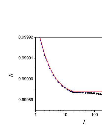
Figure 3: The differential entropy vs the length of words. The solid line is the analytical result for the correlation function $K(r)=0.01/r^{1.1}$, whereas the dots correspond to the direct numerical evaluations Eq. (22) for the numerically constructed sequence of the length $M=10^{8}$ and the cut-off parameter $r_{c}=20$. The dashed line is the differential entropy with fluctuation correction described by Eq. (28).

With increasing of $M$ (or correlations), when the inequality $K_{M}^{2}(1)>1/M$ is fulfilled, there is at list one point where the contribution of fluctuation and correlation parts of entropy are equal. For monotonically decreasing function $K(r)$ there is only one such point. Comparing the functions in square brackets in Eqs. (28) we find that they are equal at some $L=R_{s}$, which hereafter will be referred to as a stationarity length. If $L\ll R_{s}$, the fluctuations of the correlation function are negligibly small with respect to its magnitude, hence the finite sequence may be considered as quasi-stationary. At $L\sim R_{s}$ the fluctuations are of the same order as the genuine correlation function $K^{2}(r)$. Here we have to take into account the fluctuation correction due to finiteness of the random chain. At $L>R_{s}$ the fluctuating contribution exceeds the correlation one.

The other important parameter of the random sequence is the memory length $N$. If the length $N$ is less than $R_{s}$, we have no difficulties to calculate the entropy of finite sequence, which can be considered as quasi-stationary. This case is illustrated in Fig. 3. If the memory length exceeds the stationarity length $R_{s}\lesssim N$, we have to take into account the fluctuation correction to the entropy.

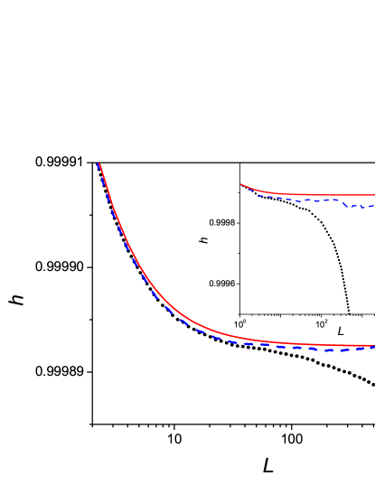
Figure 4: The differential entropy vs the length of words in $L$-axis log scale. The solid and dotted curves are the same as in the main panel of Fig. 1. The dashed line corresponds to the direct evaluations of Eq. (22) for the sequence numerically constructed by means of Eq. (14) with fluctuation correction (28) and the cut-off parameter $r_{c}=10^{4}$. The inset demonstrates the large $L$ region for the sequence of the length $M=10^{6}$.

In Fig. 4 the plot of the differential entropy versus the length of words is shown as an illustration of importance of this correction. Both numerical and analytical results are presented for the same power-law correlation function as in Figs. 1 and 3. Comparing sums of squared correlation function $K(r)=0.01/r^{1.1}$ with contribution (V), proportional to $\log_{2}[M/(M-L]$, we find that they are equal at $R_{s}\approx 10^{4}$. A graphical confirmation of this result is shown in the inset of Fig. 4. We can conclude that the dashed lines better approximate theoretical solid curves than dotted lines (till $L\approx 10^{4}$). The nonmonotone decrease of $h(L)$ is due to the fluctuation of random quantity, the entropy of the finite sequence.

VI Application to written texts

A theory of additive Markov chains with long-range memory was used for a description of correlation properties of literary texts MUYaG . The coarse-grained naturally written texts were shown to be strongly correlated sequences that possess anti-persistent properties at small distances (in the region $L\leq 300$ of grammatical rules action). At long distances (in the region $L\geq 300$ of semantic rules action) they manifest weak persistent power-law correlations. It is clear that our model of the additive Markov chain can only claim to describe the weak power-law part of entropy, proportional to $L^{-\gamma}$.

Ebeling and Nicolis EbelNic and Schürmann and Grassberger Schur suggested the empirical form of entropy for written texts

$$h_{L}=h+c\frac{\log_{2}L}{L^{\gamma}},\quad\gamma>0.$$ (29)

There emerges a natural question about the origin of this dependence. The partial answer to the question is as follows. The entropy of the Markov chain with step-wise memory function  (10) in the limit of strong correlations, $N\ln N(1-2\mu)\ll 4\mu$, was obtained in Ref. DMBUYa

$$h_{L}=h+c\frac{\log_{2}L}{L}.$$ (30)

After comparing the results of Eqs. (21) and (30) with that of Eq. (29), it becomes clear that the term $\log_{2}L$ describes strong short-range correlations and the power-law term $L^{-\gamma}$ is responsible for weak long-range correlations. So, we need a combined model that could unify two approaches of the additive Markov chain exposed above and the Markov chain with a step-wise memory function.

The answer to the question of which part of the correlation or memory function is responsible for the decimation invariance is still unsolvable.

VII Conclusion and perspectives

(i) The main result of the paper, the differential entropy of the stationary ergodic binary weakly correlated random sequence $\mathbb{A}$ is given by Eq. (22). The other important point of the work is the calculation of the fluctuation contribution to the entropy due to finiteness of random chains, the last term in Eq. (28).

(ii) In order to obtain Eq. (22) we used an assumption that the random sequence of symbols is the Markov chain. Nevertheless, the final result contains only the correlation function, does not contain the conditional probability function of the Markov chain. This allows us to suppose that result (22) and the region of its applicability is wider than the assumptions under which it is obtained Apost .

(iii) To obtain Eq. (22) we have supposed that correlations in the random chain are weak. This is not a very severe restriction. Many examples of such systems, described by means of the pair correlator are given in Ref. IzrKrMak . The randomly chosen example of DNA sequences supports this conclusion. The strongly correlated systems, which are opposed to weakly correlated chains, are nearly deterministic. For their description we need completely different approach. Their study is beyond the scope of this paper.

(iv) The developed theory opens a way for constructing a more consistent and sophisticated approach describing the systems with long-range correlations. Namely, Eq. (22) can be considered as expansion of the entropy in series with respect to the small parameter $\delta$, where the entropy $h_{0}$ of the non-correlated sequence is the zero approximation. Alternatively, for the zero approximation we can use the exactly solvable model of the $N$-step Markov chain with the conditional probability function of words occurring taken in the form of the step-wise function, Eq. (10). Another way to choose the zero approximation can be based on CPF obtained from probability of the bloc occurring Eq. (15).

(v) In this paper we have considered the random sequences with the binary space of states, but almost all results can be generalized to non-binary sequences and can be applied for describing natural written and DNA texts.

(vi) Our consideration can be generalized to the Markov chain with the infinite memory length $N$. In this case we have to impose a condition on the decreasing rate of the correlation function and the conditional probability function at $N\rightarrow\infty$.

Appendix A

Here we prove Eq. (19) using Eq. (14) as a starting point. It follows from definition (5) of the conditional probability function

$$P(1|a_{i-N+1}^{i-1})=\frac{P(a_{i-N+1}^{i-1},1)}{P(a_{i-N+1}^{i-1})}.$$ (31)

Adding the symbol $a_{i-N}$ to the string $(a_{i-N+1}^{i-1},1)$ we have

$$P(1|a_{i-N+1}^{i-1})=\frac{P(0,a_{i-N+1}^{i-1},1)+P(1,a_{i-N+1}^{i-1},1)}{P(a_{i-N+1}^{i-1})}.$$ (32)

Replacing here the probabilities $P(a_{i-N},a_{i-N+1}^{i-1},1)$ with the CPF $P(1|a_{i-N},a_{i-N+1}^{i-1})$ from equation similar to that of Eq. (31),

$$P(1|b,a_{i-N+1}^{i-1})=\frac{P(b,a_{i-N+1}^{i-1},1)}{P(b,a_{i-N+1}^{i-1})},\,\,b=(0,1),$$ (33)

after some algebraic manipulations, we get

$$P(1|a_{i-N+1}^{i-1})=\bar{a}+\sum_{r=1}^{N-1}F(r)(a_{i-r}-\bar{a})$$ (34)

$$+\frac{F(N)}{P(a_{i-N+1}^{i-1})}\left[(1-\overline{a})P(1,a_{i-N+1}^{i-1})-\overline{a}P(0,a_{i-N+1}^{i-1})\right].$$

From the compatibility condition for the Chapman-Kolmogorov equation (see, for example, Ref. gar ),

$$P(a_{i-N+1}^{i})=\sum_{a_{i-N}=0,1}P(a_{i-N}^{i-1}),P_{N}(a_{i}|a_{i-N}^{i-1}),$$ (35)

it follows that its solution is given by

$$P(k)=\overline{a}^{k}(1-\overline{a})^{N-k}+O(\delta).$$ (36)

Here $P(k)$ is the probability to have $k$ units and $(N-k)$ zeros at fixed sites of the $N$-word. Therefore, the last term in the square brackets of Eq. (34) vanishes in the main approximation, so that the difference $\left[(1-\overline{a})P(1,a_{i-N+1}^{i-1})-\overline{a}P(0,a_{i-N+1}^{i-1})\right]$ is of order of $\delta$. Hence, we have to neglect the third term in the right-hand side of Eq. (34) because it is of the second order in $\delta$. So, Eq. (19) is proven for $L=N-1$. By induction the equation can be written for arbitrary $L$.

References

- (1) P. Ehrenfest, T. Ehrenfest, Encyklopädie der Mathematischen Wissenschaften (Springer, Berlin, 1011), p. 742, Bd. II.
- (2) D. Lind and B. Marcus. An Introduction to Symbolic Dynamics and Coding (Cambridge University Press, Cambridge, 1995).
- (3) T. M. Cover, J. A. Thomas, Elements of Information Theory (Wiley, New York, 1991).
- (4) F. M. Izrailev, A. A. Krokhin, N. M. Makarov, Phys. Rep. 512, 125 (2012).
- (5) C. E. Shannon and W. Weaver, The Mathematical Theory of Communication (University of Illinois Press, Urbana, Illinois, 1949).
- (6) A. N. Shiryaev, Probability (Springer, New York, 1996).
- (7) S. S. Melnyk, O. V. Usatenko, V. A. Yampol’skii, Physica A 361, 405 (2006).
- (8) O. V. Usatenko, S. S. Apostolov, Z. A. Mayzelis, and S. S. Melnik, Random finite-valued dynamical systems: additive Markov chain approach (Cambridge Scientific Publisher, Cambridge, 2010).
- (9) S. S. Melnyk, O. V. Usatenko, V. A. Yampol’skii, V. A. Golick, Phys. Rev. E 72, 026140 (2005).
- (10) S. S. Apostolov, Z. A. Mayzelis, O. V. Usatenko, V. A. Yampol’skii, Int. J. Mod. Phys. B 22, 3841 (2008).
- (11) O. V. Usatenko, V. A. Yampol’skii, Phys. Rev. Lett. 90, 110601 (2003).
- (12) W. Ebeling and G. Nicolis, Europhys. Lett. 14, 191 (1991).
- (13) T. Schürmann and P. Grassberger, Chaos 6, 414 (1996).
- (14) S. Denisov, S. S. Melnik, A. A. Borisenko, O. V. Usatenko, and V. A. Yampolsky (unpublished).
- (15) C. W. Gardiner, Handbook of Stochastic Methods for Physics, Chemistry, and the Natural Sciences, Springer Series in Synergetics, Vol. 13 (Springer-Verlag, Berlin, 1985).
- (16) S.A. Apostiolov (private communication).