Acoustic integrated extinction

Abstract

The integrated extinction (IE) is defined as the integral of the scattering cross-section as a function of wavelength. Sohl et al. [1] derived an IE expression for acoustic scattering that is causal, i.e.  the scattered wavefront in the forward direction arrives later than the incident plane wave in the background medium. The IE formula was based on electromagnetic results, for which scattering is causal by default. Here we derive a formula for the acoustic IE that is valid for causal and non-causal scattering. The general result is expressed as an integral of the time dependent forward scattering function. The IE reduces to a finite integral for scatterers with zero long-wavelength monopole and dipole amplitudes. Implications for acoustic cloaking are discussed and a new metric is proposed for broadband acoustic transparency.

1 Introduction

The optical theorem, which relates the total scattering cross section of time harmonic waves to the forward scattering amplitude, is a well known and useful relation for acoustic, electromagnetic and elastic waves, e.g.  [2] derives the optical theorem for both acoustics and elastodynamics. Another powerful general identity is for the integrated extinction, (IE), an integral of the scattering cross-section over all wavelengths, which is a useful measure of the total scattering strength of an acoustic target. The concept of integrated extinction was introduced in 1969 by Purcell [3] in relation to optical scattering from interstellar grains. The IE is proportional to a linear combination of the monopole and dipole amplitudes if the scattering is causal [1], that is, the wavefront of the scattered response in the forward Fvers direction arrives after an equivalent plane wavefront in the background medium. Causal scattering is the default in electromagnetics since nothing travels faster than light in a vacuum; but there is no such limitation in acoustics. Many scattering situations of interest in acoustics are non-causal, such as metal objects in water or air, for which the IE expression of [1] does not apply.

Our objective in this paper is an expression for the acoustic integrated extinction that is valid under all circumstances, one that is not restricted to causal or non-causal scatterers. Previous forms of the causal identity for the IE have been cast in terms of the the frequency domain function that defines the forward scattering amplitude [1]. We find it more useful, particularly for non-causal scattering, to phrase results in terms of the time dependent forward scattering function which is the inverse Fourier transform of the frequency domain function. [4] considered EM forward scattering sum rules in the time domain, including the IE formula, however, the results are restricted to causal scattering and therefore not transferable to acoustics. Note: the adjective ”causal” is used here in the same sense as in [1]. Terms such as ”post-scattering”, ”subsonic” could be used; however ”causal” is preferred because of its connection with analytic properties of complex-valued functions, which will be used later.

The integrated extinction is a measure of total scattering strength over all frequencies which serves as a natural metric for measuring reduction in scattering using physical mechanisms [5, 6]. The general expressions for IE derived in this paper provide new interpretations for reduction of acoustic scattering. In contrast to the electromagnetic situation, it is possible to have the formal IE expression for causal acoustic scattering to become zero. We show that this is possible iff the acoustic scatterer is non-causal. An important example of such an acoustic scatterer is the neutral acoustic inclusion, which by definition has zero monopole and dipole scattered amplitudes. Based upon the IE results derived in this paper we explore the relationships between integrated extinction, neutral acoustic inclusions, cloaking and causality.

The outline of the paper is as follows. In §2 the scattering cross-section and integrated extinction are defined and the result of [1], originally given for 3-dimensional scattering is presented for causal acoustic scattering in one, two and three dimensions. The main result for the IE is derived in §3. Examples are given in §4 for scattering in a one dimensional system for which the IE can be found in explicit form.

2 Scattering cross section and integrated extinction

Let $p({\bf x})$ be the complex-valued acoustic pressure in a fluid of uniform density $\rho$ and compressibility $C$ (or its inverse the bulk modulus $K=C^{-1}$) outside of a finite region $\Omega$, the scatterer. It satisfies the Helmholtz equation

$$\nabla^{2}p+k^{2}p=0,\ \ {\bf x}\not\in\Omega,$$ (1)

where $k=\omega/c$, $\omega$ is frequency and $c=1/\sqrt{C\rho}$ is the sound speed. Time harmonic dependence is considered with the factor $e^{-i\omega t}$ understood and omitted. The system may be one, two or three-dimensional.

The total field is an incident plane wave plus the scattered pressure: $p=p_{0}e^{ikx}+p_{s}$ ($p_{0}$ constant). Introduce the far-field scattering amplitude $S(\theta,\omega)$ where $\theta$ defines the scattering direction, $\theta=0$ corresponding to the direction of incidence $\hat{\bf k}$, and

$$p_{s}({\bf x})=p_{0}\,S(\theta,\omega)\,\big{[}k/(i2\pi|{\bf x}|)\big{]}^{\frac{d-1}{2}}\,e^{ik|{\bf x}|},\ \ |{\bf x}|\to\infty$$ (2)

where $d=1$, $2$ or $3$ is the dimension. Equation (2) is exact in 1D $(d=1)$ for all ${\bf x}\not\in\Omega$ in which case $T=1+S(0,\omega)$ and $R=S(\pi,\omega)$ are the transmission and reflection coefficients, respectively, satisfying $|R|^{2}+|T|^{2}=1$. Define the total scattering cross section $\sigma$ (also known as the extinction)

$$\sigma(\omega)=|p_{0}|^{-2}\,\int|p_{s}|^{2}\operatorname{d}s$$ (3)

where the integral is around a closed surface enclosing the scatterer. Conservation of energy requires zero total energy flux across the closed surface, which implies the ”optical theorem” relating $\sigma$ to the forward scattering

$$\sigma=-2\,\operatorname{Re}S(\omega)\ \ \text{where}\ S(\omega)\equiv S(0,\omega).$$ (4)

Our focus is on the integrated extinction, defined as

$$\operatorname{\Sigma}\equiv\int_{0}^{\infty}\frac{\sigma(\omega)}{\omega^{2}}\,\operatorname{d}\omega.$$ (5)

This is clearly a measure of the total scattering strength over all frequencies. It is worth noting that $\sigma$ typically tends to a constant non-zero value as $\omega\to\infty$ while $\sigma={\cal O}(\omega^{2})$ for $\omega\to 0$ (although see the remark after eq (38)). Hence the only integer value $n$ for which the integral $\text{I}=\int_{0}^{\infty}\omega^{-n}\sigma\operatorname{d}\omega$ is bounded, and therefore meaningful, is $n=2$, i.e.  $\text{I}=\operatorname{\Sigma}$. The IE can also be expressed as an integral over wavelength $\lambda=2\pi c/\omega$,

$$\operatorname{\Sigma}=\frac{1}{2\pi c}\int_{0}^{\infty}\sigma\,\operatorname{d}\lambda.$$ (6)

Causality for the forward scatter is defined such that wave motion in the forward direction does not precede signals from the otherwise uniform medium. This implies that $S(\omega)$ is analytic in the upper half of the complex $\omega-$plane. The transform $f(\omega)$ of any such causal function satisfies the Sokhotski-Plemelj relations for real values of $\omega$ [7, eq. (1.6.11)]

$$f(\omega)=\frac{1}{i\pi}\mathchoice{{\vbox{\hbox{$\textstyle-$}}\kern-4.86108pt}}{{\vbox{\hbox{$\scriptstyle-$}}\kern-3.25pt}}{{\vbox{\hbox{$\scriptscriptstyle-$}}\kern-2.29166pt}}{{\vbox{\hbox{$\scriptscriptstyle-$}}\kern-1.875pt}}\!\int_{-\infty}^{\infty}\frac{f(\omega^{\prime})\operatorname{d}\omega^{\prime}}{\omega^{\prime}-\omega},$$ (7)

where $\mathchoice{{\vbox{\hbox{$\textstyle-$}}\kern-4.86108pt}}{{\vbox{\hbox{$\scriptstyle-$}}\kern-3.25pt}}{{\vbox{\hbox{$\scriptscriptstyle-$}}\kern-2.29166pt}}{{\vbox{\hbox{$\scriptscriptstyle-$}}\kern-1.875pt}}\!\int$ denotes principal value integral. Setting $f(\omega)=S(\omega)/\omega$, and using $\sigma(-\omega)=\sigma(\omega)$, it follows that

$$\operatorname{\Sigma}=\operatorname{\Sigma}_{\text{pc}}\ \ \text{where}\ \ \operatorname{\Sigma}_{\text{pc}}\equiv\pi\operatorname{Im}\left.\frac{S(\omega)}{\omega}\right|_{\omega=0}$$ (8)

and ”pc” is included to emphasize that this result is strictly limited to purely causal forward scattering. Equation (8), originally derived in [1] for 3D, is here generalized to include the 1D and 2D cases. We note that eq. (8) also follows from the fact that $-iS(\omega)$ is a Herglotz function [8].

The zero frequency limit in (8) allows us to interpret $\operatorname{\Sigma}_{\text{pc}}$ in terms of quasistatic properties. Thus, if the scatterer is a region of volume $V$ with uniform density $\rho^{\prime}$ and compressibility $C^{\prime}({\bf x})$, then [1]

$$\operatorname{\Sigma}_{\text{pc}}=\frac{\pi}{2c}\Big{(}\big{(}\frac{\langle C^{\prime}\rangle}{C}-1\big{)}V-\hat{\bf k}\cdot{\boldsymbol{\gamma}}\Big{(}\frac{\rho}{\rho^{\prime}}\Big{)}\cdot\hat{\bf k}\Big{)}$$ (9)

where ${\boldsymbol{\gamma}}$ is the polarizability dyadic [2] proportional to $V$ and $\langle C^{\prime}\rangle$ is the average compressibility.

As noted in [1], the identity (8) is only valid for causal scattering. Next, we show how to extend these results to non-causal scattering.

3 Integrated extinction for non-causal scattering

Assuming the forward scattering is non-causal, we may distinguish its causal and anti-causal components $s_{+}(t)$ and $s_{-}(t)$, respectively, as

$$s(t)\equiv\frac{1}{2\pi}\int_{-\infty}^{\infty}S(\omega)e^{-i\omega t}\operatorname{d}\omega=s_{-}(t)+s_{+}(t),\ \ s_{\pm}(t)=0\ \text{for}\ t^{<}_{>}0.$$ (10)

Thus, $s(t)=0$ for $t<0$ if the scattering is causal, while for non-causal scattering there is some finite time before $t=0$ for which $s(t)\neq 0$. The time dependent function $s(t)$ can be identified as a forward scattered “impulse-response” function corresponding to an incident delta pulse $p_{\text{inc}}(x,t)=p_{0}\delta(t-x/c)$. Subscripts $\pm$ denote functions that are causal/anti-causal, with Fourier transforms analytic in the upper and lower half planes, respectively. The frequency dependent forward scattering function decomposes as

$$S(\omega)=S_{-}(\omega)+S_{+}(\omega),$$ (11)

where

$$S_{\pm}(\omega)=\int_{0}^{\infty}s_{\pm}(\pm t)e^{\pm i\omega t}\operatorname{d}t.$$ (12)

Causal scattering corresponds to $s_{-}(t)=0$ $\Leftrightarrow$ $S_{-}(\omega)=0$; in the non-causal case both $s_{-}$ and $S_{-}$ are non-zero.

We note the generalization of the Sokhotski-Plemelj relations (7),

$$\big{(}\operatorname{Re}f_{\pm}(\omega),\,\operatorname{Im}f_{\pm}(\omega)\big{)}=\pm\frac{1}{\pi}\mathchoice{{\vbox{\hbox{$\textstyle-$}}\kern-4.86108pt}}{{\vbox{\hbox{$\scriptstyle-$}}\kern-3.25pt}}{{\vbox{\hbox{$\scriptscriptstyle-$}}\kern-2.29166pt}}{{\vbox{\hbox{$\scriptscriptstyle-$}}\kern-1.875pt}}\!\int_{-\infty}^{\infty}\big{(}\operatorname{Im}f_{\pm}(\omega^{\prime}),\,-\operatorname{Re}f_{\pm}(\omega^{\prime})\big{)}\frac{\operatorname{d}\omega^{\prime}}{\omega^{\prime}-\omega}$$ (13)

for $\omega$ real. Hence, using (11),

$$-\frac{1}{\pi}\mathchoice{{\vbox{\hbox{$\textstyle-$}}\kern-4.86108pt}}{{\vbox{\hbox{$\scriptstyle-$}}\kern-3.25pt}}{{\vbox{\hbox{$\scriptscriptstyle-$}}\kern-2.29166pt}}{{\vbox{\hbox{$\scriptscriptstyle-$}}\kern-1.875pt}}\!\int_{-\infty}^{\infty}\operatorname{Re}S(\omega)\frac{\operatorname{d}\omega}{\omega^{2}} =\left.\operatorname{Im}\frac{S_{+}(\omega)}{\omega}\right|_{\omega=0+i0}-\left.\operatorname{Im}\frac{S_{-}(\omega)}{\omega}\right|_{\omega=0-i0}$$

$$=\left.\operatorname{Im}\frac{S(\omega)}{\omega}\right|_{\omega=0}-\lim_{\epsilon\to 0}\operatorname{Im}\bigg{(}\frac{S_{-}(i\epsilon)}{i\epsilon}+\frac{S_{-}(-i\epsilon)}{-i\epsilon}\bigg{)}.$$ (14)

This gives us the first form of our main result:

$$\boxed{\operatorname{\Sigma}=\pi\operatorname{Im}\bigg{(}\left.\frac{S(\omega)}{\omega}\right|_{\omega=0}-2\frac{\operatorname{d}S_{-}}{\operatorname{d}\omega}(0)\bigg{)}.}$$ (15)

The second term involving $S_{-}$vanishes if the scattering is causal, recovering the results of [1]. The relationship (15) can be written in alternative form

$${\operatorname{\Sigma}=\pi\operatorname{Im}\bigg{(}\frac{\operatorname{d}S_{+}}{\operatorname{d}\omega}(0)-\frac{\operatorname{d}S_{-}}{\operatorname{d}\omega}(0)\bigg{)}}$$ (16)

emphasizing the similar contributions from the causal and non-causal components of the forward scattered response. With hindsight, the identity (16) follows more directly by noting that $\operatorname{\Sigma}$ may be defined

$$\operatorname{\Sigma}=\int_{0}^{\infty}\frac{\operatorname{d}\sigma}{\operatorname{d}\omega}\,\frac{\operatorname{d}\omega}{\omega},$$ (17)

which follows from (5) using the fact that $\lim_{\omega\to 0}\sigma/\omega=0$.

The identity (16) does not have an obvious interpretation in terms of quasi-static quantities, unlike its causal version eqs. (8) and (9). However, if we represent (16) in the time domain, which is easily done using the definition of the Fourier transform, we find

$$\boxed{\operatorname{\Sigma}=\pi\int_{-\infty}^{\infty}|t|\,s(t)\operatorname{d}t.}$$ (18)

This result applies for causal and non-causal scattering. Note the appearance of $|t|$ in (18). The same integral with $|t|$ replaced by $t$ is simply

$$\int_{-\infty}^{\infty}t\,s(t)\operatorname{d}t=\operatorname{Im}\left.\frac{S(\omega)}{\omega}\right|_{\omega=0}.$$ (19)

Hence, eqs. (8), (18) and (19) imply that the integrated extinction can be written

$$\boxed{\operatorname{\Sigma}=\operatorname{\Sigma}_{\text{pc}}-2\pi\int_{-\infty}^{0}t\,s(t)\operatorname{d}t.}$$ (20)

This particular form of the integrated extinction identity generalizes the causal-only result (8). Note that the non-causal response is zero for some $t_{-}<0$, i.e. $s(t)=0$, $t<t_{-}$, and hence the integral in (20) is only over a finite interval of time from $t_{-}$ to $0$.

4 Examples

4.1 Arbitrarily layered one dimensional medium

Consider a 1D system with non-uniform density and compressibility $\rho^{\prime}(x)$, $C^{\prime}(x)$ restricted to $\Omega=[0,a]$. The forward scattering amplitude is

$$S(\omega)=-1+2e^{-ika}/\big{(}M_{11}+M_{22}-zM_{12}-z^{-1}M_{21}\big{)}$$ (21)

where $z=\rho c$ is the background acoustic impedance and $M_{ij}$ are elements of the 2$\times$2 propagator matrix ${\bf M}(a)$, $\det{\bf M}=1$, the solution to

$$\frac{\operatorname{d}{\bf M}(x)}{\operatorname{d}x}=i\omega{\bf Q}{\bf M},\ \ {\bf M}(0)={\bf I},$$ (22)

with ${\bf I}$ the identity and

$${\bf Q}(x)=\begin{pmatrix}0&C^{\prime}(x)\\ \rho^{\prime}(x)&0\end{pmatrix}.$$ (23)

The solution (21) follows using standard methods for uni-dimensional systems. For our purposes, we note that at low frequency ${\bf M}(a)={\bf I}+i\omega a\langle{\bf Q}\rangle+...$ where $\langle\cdot\rangle$ denotes the average value in $\Omega$.

Define the non-dimensional travel time

$$\operatorname{T}=\frac{c}{a}\int_{0}^{a}\frac{\operatorname{d}x}{c^{\prime}(x)}$$ (24)

which is the ratio of the travel time across the inhomogeneous region to the travel time across an equivalent uniform slab. The slab has the same travel time as the equivalent uniform slab if $\operatorname{T}=1$; hence the scatterer is causal if $\operatorname{T}\geq 1$, and non-causal otherwise. Next, we consider the causal and non-causal cases separately.

For causal scattering ($\operatorname{T}\geq 1$) the integrated extinction is simply, using eq. (8),

$$\operatorname{\Sigma}_{\text{pc}}=\frac{\pi}{2}\frac{a}{c}\Big{(}\frac{\big{\langle}C^{\prime}\rangle}{C}+\frac{\langle\rho^{\prime}\rangle}{\rho}-2\Big{)}.$$ (25)

It is then a straightforward calculation to show that

$$\operatorname{\Sigma}_{\text{pc}}={\pi}\frac{a}{c}\bigg{(}\frac{1}{2}\Big{\langle}\frac{c}{c^{\prime}}\Big{(}\sqrt{\frac{z^{\prime}}{z}}-\sqrt{\frac{z}{z^{\prime}}}\Big{)}^{2}\Big{\rangle}+\operatorname{T}-1\bigg{)}$$ (26)

where $z^{\prime}=\rho^{\prime}c^{\prime}$ is the impedance. Since the scatterer is causal $(\operatorname{T}\geq 1)$ this means that $\operatorname{\Sigma}_{\text{pc}}\geq 0$ with equality iff $\operatorname{T}=1$ and the local impedance is constant and equal to the uniform impedance, i.e. $z^{\prime}=z$. In summary, it is possible that the total IE of eq. (25) can vanish, but only if the slab has (i) uniform impedance and (ii) travel time equivalent to the uniform medium. Condition (i) is expected, it guarantees no reflection/back-scattering, while (ii) ensures that the phase of the transmitted wave is the same as that for the uniform medium.

Note that the expression in the right hand side of (26) can vanish for a non-constant impedance if

$$\operatorname{T}=1-\frac{1}{2}\big{\langle}\Big{(}\big{(}\frac{\rho^{\prime}}{\rho}\big{)}^{1/2}-\big{(}\frac{C^{\prime}}{C}\big{)}^{1/2}\Big{)}^{2}\big{\rangle}\leq 1.$$ (27)

However, (26) no longer represents the IE in this case since the scattering is non-causal $(\operatorname{T}<1)$ and therefore $\operatorname{\Sigma}\neq\operatorname{\Sigma}_{\text{pc}}$. That is, satisfaction of (27) does not imply that the integrated extinction vanishes.

An expression for the IE under both causal and non-causal conditions can be found if the impedance is everywhere constant. The transmitted wave is then of unit amplitude with phase defined by $\operatorname{T}$ of (24), and therefore $S(\omega)=-1+e^{-ika}e^{ika\operatorname{T}}$. The split functions are $S_{+}(\omega)=S(\omega)$, $S_{-}(\omega)=0$ if $\operatorname{T}\geq 1$, and $S_{+}(\omega)=0$, $S_{-}(\omega)=S(\omega)$ if $\operatorname{T}<1$, from which the IE follows using eq. (16) as

$$\operatorname{\Sigma}={\pi}\frac{a}{c}\,|\operatorname{T}-1|\ \ \text{for constant impedance}.$$ (28)

4.2 A uniform layer

A layer with material properties $\rho^{\prime}$, $C^{\prime}$ occupies $x\in[0,a]$ in the otherwise uniform background. Then, setting $k^{\prime}=\omega/c^{\prime}$, $c^{\prime}=1/\sqrt{\rho^{\prime}C^{\prime}}$, $z^{\prime}=\rho^{\prime}c^{\prime}$,

$$S(\omega)=-1+4z{z^{\prime}}e^{-ika}\big{(}({z^{\prime}}+z)^{2}e^{-ik^{\prime}a}-({z^{\prime}}-z)^{2}e^{ik^{\prime}a}\big{)}^{-1}$$ (29)

from which the forward scattering impulse response is found

$$s(t)=-\delta(t)+\frac{4zz^{\prime}}{(z^{\prime}-z)^{2}}\sum_{n=1}^{\infty}\big{(}\frac{z^{\prime}-z}{z^{\prime}+z}\big{)}^{2n}\delta(t-t_{n}),\ \ t_{n}=(2n-1)\frac{a}{c^{\prime}}-\frac{a}{c}.$$ (30)

If the layer is non-causal, let $N\geq 1$ be the number of non-causal pulses, i.e. $t_{N}=$max$\,t_{n}$, $t_{n}<0$, then eqs. (11) and (30) yield

$$S_{-}(\omega)=\frac{4zz^{\prime}}{(z^{\prime}-z)^{2}}\sum_{n=1}^{N}\big{(}\frac{z^{\prime}-z}{z^{\prime}+z}\big{)}^{2n}\,e^{i\omega t_{n}}.$$ (31)

This may be summed to give

$$S_{-}(\omega)=\big{(}S(\omega)+1\big{)}\,\Big{(}1-\Big{[}\Big{(}\frac{z^{\prime}-z}{z^{\prime}+z}\Big{)}e^{i\omega\frac{a}{c^{\prime}}}\Big{]}^{2N}\Big{)}.$$ (32)

We now give three different expressions for the integrated extinction based on the equivalent identities (15), (18) and (20). The first formula for $\operatorname{\Sigma}$ corresponds to eqs.  (18) and it follows directly using eq. (30),

$$\operatorname{\Sigma}=\frac{4\pi zz^{\prime}}{(z^{\prime}-z)^{2}}\sum_{n=1}^{\infty}\big{(}\frac{z^{\prime}-z}{z^{\prime}+z}\big{)}^{2n}\,|t_{n}|.$$ (33)

The strictly causal expression for $\operatorname{\Sigma}$ is given by eq. (25), and the non-causal variant follows from the part of $s(t)$ of (30) that is non-zero for negative time, i.e. for $t_{n}<0$. Combining these yields an alternative expression for $\operatorname{\Sigma}$ corresponding to eq.  (20),

$$\operatorname{\Sigma}=\frac{\pi}{2}\bigg{(}\Big{(}\frac{z}{z^{\prime}}+\frac{z^{\prime}}{z}\Big{)}\frac{a}{c^{\prime}}-2\frac{a}{c}-16\frac{z}{z^{\prime}}\big{(}1-\frac{z}{z^{\prime}}\big{)}^{-2}\sum_{n=1}^{N}\Big{(}\frac{z^{\prime}-z}{z^{\prime}+z}\Big{)}^{2n}\,t_{n}\,H(-t_{1})\bigg{)}$$ (34)

where $H$ is the Heaviside step function. Finally, using eq. (32), the formula (15) becomes for this example

$$\operatorname{\Sigma}=\frac{\pi}{2}\Big{(}\Big{(}\frac{z}{z^{\prime}}+\frac{z^{\prime}}{z}+4N\Big{)}\frac{a}{c^{\prime}}-2\frac{a}{c}\Big{)}\Big{(}2\Big{(}\frac{z^{\prime}-z}{z^{\prime}+z}\Big{)}^{2N}-1\Big{)}+2\pi N\frac{a}{c^{\prime}}.$$ (35)

The three expressions (33), (34) and (35) for $\operatorname{\Sigma}$ are obviously equivalent, and are each valid whether the scattering is causal or non-causal. Equation (33) gives the integrated extinction as an infinite sum, eq. (34) replaces the infinite sum with a finite one, and eq. (35) provides the most compact version. Note that the simpler result for causal scattering, i.e. eq. (25), is evident from eqs. (34) and (35), corresponding to $N=0$ in the latter. The parameter $N$ is a positive integer for non-causal scattering. This might suggest that the expressions (34) and (35) behave discontinuously as a function of the slab speed $c^{\prime}$, which defines $N$. However, this is not the case as can be seen from the fact that as $N$ increases or decreases by unity, one additional value of $t_{n}$ is zero as it becomes negative or positive, respectively. The identities (33) and (34) are then clearly continuous functions of $c^{\prime}$, as must be eq. (35).

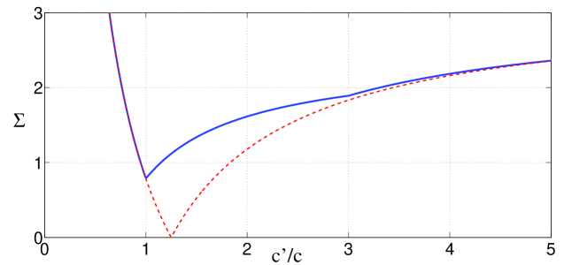
Figure 1: The solid curve shows $\operatorname{\Sigma}$ as a function of $c^{\prime}/c$ for a uniform slab $z^{\prime}/z=2$, $a/c=1$. The dashed curve shows the magnitude of the causal integrated extinction defined in (36).

4.3 Numerical example

The integrated extinction for a uniform slab with impedance twice the background value $(z^{\prime}=2z)$ is shown in Figure 1 as a function of the slab wave speed. Also shown is the magnitude of the purely causal IE (see eq. (25))

$$\operatorname{\Sigma}_{\text{pc}}=\frac{\pi a}{2c}\Big{(}\Big{(}\frac{z}{z^{\prime}}+\frac{z^{\prime}}{z}\Big{)}\frac{c}{c^{\prime}}-2\Big{)}.$$ (36)

Clearly, $\operatorname{\Sigma}=\operatorname{\Sigma}_{\text{pc}}$ for $c^{\prime}\leq c$ as expected. However, it is also evident that $\operatorname{\Sigma}\approx-\operatorname{\Sigma}_{\text{pc}}$ for $c^{\prime}>3c$ with the approximation better as $c^{\prime}$ becomes larger. The reason for this can be understood from the mathematical form of $\operatorname{\Sigma}$ in eq. (35). The number $N$ increases approximately linearly with the slab speed $c^{\prime}$when all other slab parameters are held fixed. The quantity $(\frac{z^{\prime}-z}{z^{\prime}+z})^{2N}$ therefore decreases with increasing $c^{\prime}$, so that $\operatorname{\Sigma}\to-\operatorname{\Sigma}_{\text{pc}}$ as this quantity tends to zero.

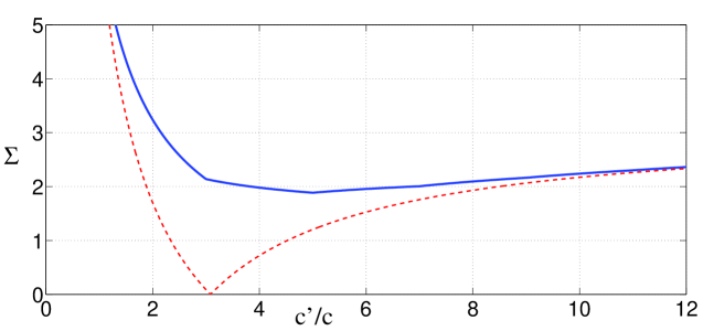
Figure 2: The curves are the same as in Figure 1 except that the slab impedance is $z^{\prime}=6z$.

Figure 2 shows the same phenomenon for a larger slab impedance $(z^{\prime}/z=6)$. The limiting behavior $\operatorname{\Sigma}\approx-\operatorname{\Sigma}_{\text{pc}}$ is again observed, this time at larger values of $c^{\prime}$ since the quantity $(\frac{z^{\prime}-z}{z^{\prime}+z})^{2N}$ decreases less rapidly than for Figure 1. Note that the same curves are obtained in Figures 1 and 2 for $z/z^{\prime}=2$ and $z/z^{\prime}=6$, respectively, since eq. (35) is unchanged for $\frac{z^{\prime}}{z}\leftrightarrow\frac{z}{z^{\prime}}$.

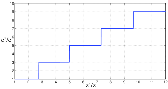
Figure 3: The curve shows the value of slab wave speed $c^{\prime}$ which minimizes the integrated extinction of eq. (35) for given values of slab impedance $z^{\prime}\geq z$, and fixed slab thickness.

The simple form of the expression for the purely causal IE in eq. (36) indicates that for a given value of the slab impedance, $z^{\prime}$, the minimum value of $\operatorname{\Sigma}_{\text{pc}}$ for all possible slab wave speeds $c^{\prime}\leq c$ is achieved at $c^{\prime}=c$. Conversely, for a given value of $c^{\prime}<c$, the minimum value of $\operatorname{\Sigma}_{\text{pc}}$ is achieved at $z^{\prime}=z$. The location of the minimizing values of the dual parameter at the edges $c^{\prime}=c$, $z^{\prime}=z$ suggest that these IE values are not necessarily the global minima. Figure 3 shows, as expected, that the global minimum of IE for a given slab impedance is achieved by a non-causal slab wave speed. The minimizing value of $c^{\prime}/c$ is an odd integer greater than or equal to unity, the value of which is a discontinuous function of $z^{\prime}/z$ that increases monotonically in a roughly linear manner. The complicated nature of this function is displayed in Figure 4 which shows the minimizing value of the slab density as a function of slab impedance.

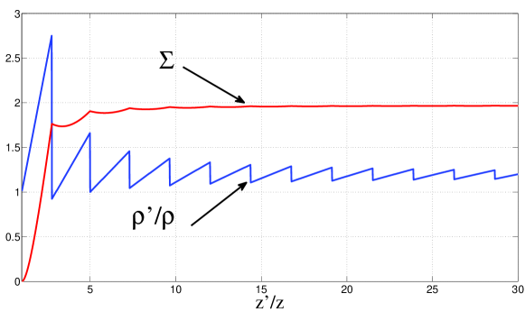
Figure 4: For given values of slab impedance $z^{\prime}\geq z$ and $a/c=1$, the blue curve shows the value of slab density $\rho^{\prime}$ which minimizes the integrated extinction of eq. (35). The red curve is the corresponding minimal value of $\operatorname{\Sigma}$.

4.4 Two and three dimensions

Consider plane wave incidence on a uniform circular $(d=2)$ or spherical $(d=3)$ inhomogeneity of radius $a$ and properties $C^{\prime}$, $\rho^{\prime}$. The low frequency expansion of the forward scattering amplitude follows, using standard methods, as

$$S(\omega)=i\omega\pi\frac{(d-1)}{d}\,\frac{a^{d}}{c}\Big{[}\frac{C^{\prime}}{C}-1+\frac{d\big{(}\frac{\rho^{\prime}}{\rho}-1\big{)}}{(d-1)\frac{\rho^{\prime}}{\rho}+1}\Big{]}+{\cal O}(\omega^{2}).$$ (37)

The IE for causal scattering then follows from eqs. (8) and (37) as

$$\operatorname{\Sigma}_{\text{pc}}=\pi^{2}\frac{(d-1)}{d}\,\frac{a^{d}}{c}\,\frac{\rho}{\rho^{\prime}}\bigg{(}\frac{\big{(}\frac{\rho^{\prime}}{\rho}-1\big{)}^{2}}{(d-1)\frac{\rho^{\prime}}{\rho}+1}+\operatorname{T}^{2}-1\bigg{)}$$ (38)

where $\operatorname{T}=(\rho^{\prime}C^{\prime})^{1/2}/c$ is the ratio of travel times. It is interesting to compare this with the analogous 1D result eq. (26). Since $\operatorname{T}\geq 1$ for causal scattering, eq. (38) shows that $\operatorname{\Sigma}_{\text{pc}}$ vanishes iff $\rho^{\prime}=\rho$, $C^{\prime}=C$, implying that there is no combination of $\rho^{\prime}$, $C^{\prime}$ that is transparent except for the trivial case when the scatterer is identical with the background acoustic fluid.

The causal IE of eq. (38) tends to infinity as the compressibility $C^{\prime}$ of the scatterer becomes infinite. This limit can be identified with pressure release boundary conditions: $p=0$ on $r=a$, for which the scattering cross-section of the sphere tends to a non-zero constant as $\omega\to 0$, specifically $\sigma=4\pi a^{2}\big{[}1+\frac{1}{3}(ka)^{2}+{\cal O}\big{(}(ka)^{4}\big{)}\big{]}$ [9]. The IE as defined in eq. (5) is not integrable at $\omega=0$ and therefore not applicable to scatterers with pressure-release boundaries. However, such boundary conditions are not strictly physical since a fluid with a pressure-release inclusion is not stable under static pressure perturbation: the hole collapses. This non-physical limit is apparent in the finite scattering cross-section of the sphere at zero frequency.

5 Discussion

5.1 The limiting cases $\operatorname{\Sigma}=\operatorname{\Sigma}_{\text{pc}}$ and $\operatorname{\Sigma}\approx-\operatorname{\Sigma}_{\text{pc}}$

The above results suggest separation of the integrated extinction as distinct contributions

$$\operatorname{\Sigma}^{(+)} =\pi\int_{0}^{\infty}t\,s(t)\operatorname{d}t=\pi\operatorname{Im}\frac{\operatorname{d}S_{+}}{\operatorname{d}\omega}(0),$$ (39)

$$\operatorname{\Sigma}^{(-)} =-\pi\int_{-\infty}^{0}t\,s(t)\operatorname{d}t=-\pi\operatorname{Im}\frac{\operatorname{d}S_{-}}{\operatorname{d}\omega}(0).$$

$\operatorname{\Sigma}^{(+)}$ and $\operatorname{\Sigma}^{(-)}$ can be considered as causal and non-causal parts of the IE, respectively, through the relation of the IE to the forward scattering. Their connection with the general and the purely causal expressions for the IE follow from eqs. (16), (18) and (20),

$$\operatorname{\Sigma} =\operatorname{\Sigma}^{(+)}+\operatorname{\Sigma}^{(-)},$$ (40)

$$\operatorname{\Sigma}_{\text{pc}} =\operatorname{\Sigma}^{(+)}-\operatorname{\Sigma}^{(-)}.$$

The IE can be expressed in the suggestive forms

$$\operatorname{\Sigma} =\operatorname{\Sigma}_{\text{pc}}+2\operatorname{\Sigma}^{(-)}$$ (41)

$$=-\operatorname{\Sigma}_{\text{pc}}+2\operatorname{\Sigma}^{(+)}.$$

The identity of Sohl et al. [1] in eq. (8) for purely causal scattering follows from the first of these with $\operatorname{\Sigma}^{(-)}=0$. A major point of this paper is that the scattering can be mainly non-causal in the sense of the examples in Figures 1 and 2. This can occur in one, two or three dimensions if the scatterer supports very fast waves relative to the background, e.g.  metallic scatterers in air. If the non-causal scattering predominates then most of the incident energy is scattered before $t=0$, implying $|\operatorname{\Sigma}^{(-)}|\gg|\operatorname{\Sigma}^{(+)}|$ and therefore

$$\operatorname{\Sigma}\approx-\operatorname{\Sigma}_{\text{pc}}.$$ (42)

Relation (42) is essentially the opposite of the causal identity (8). Introduce a new quantity, $\operatorname{\Sigma}_{\text{pnc}}\equiv-\operatorname{\Sigma}_{\text{pc}}$, then it is clear that $\operatorname{\Sigma}_{\text{pnc}}$ is the IE for purely non-causal scattering. It should be borne in mind that the approximation (42) becomes precise only in the limit that the scatterer supports waves of infinite speed, which is not possible in acoustics because it requires either zero material density or compressibility. Of course, infinite wave speed is prohibited in electromagnetics, although for a different reason.

5.2 Neutral acoustic inclusions and cloaking

For purely causal scattering, as in electromagnetics, the IE must be positive definite and hence the forward scattering amplitude on the right hand side of (9) must be positive. This constraint does not apply in acoustics. The multipole expansion of the scattering function $S(\theta,\omega)$ at low frequency (long wavelength) is a power series in $\omega$, hence the low frequency limit of the forward scatter is necessarily defined by the first few multipole terms. A neutral acoustic inclusion by definition has zero monopole and dipole scattered amplitudes. The two terms in the expression (9) for $\operatorname{\Sigma}_{\text{pc}}$ correspond to the monopole and dipole contribution to the forward scatter. Specifically, the monopole amplitude is proportional to $\big{(}\frac{\langle C^{\prime}\rangle}{C}-1\big{)}V$ while the dipole amplitude depends on the polarizability tensor ${\boldsymbol{\gamma}}$. Both terms are identically zero for a neutral acoustic inclusion, implying that $\operatorname{\Sigma}_{\text{pc}}=0$.

Hence, a neutral acoustic inclusion is a non-causal scatterer. By definition

$$\int_{-\infty}^{\infty}t\,s(t)\operatorname{d}t=0\ \ \text{for a neutral acoustic inclusion},$$ (43)

which follows from eqs. (8) and (19). Combining eqs. (18) and (43) yields

$$\operatorname{\Sigma}=-2\pi\int_{-\infty}^{0}t\,s(t)\operatorname{d}t\ \ \text{for a neutral acoustic inclusion}.$$ (44)

The integrated extinction of a neutral acoustic inclusion is therefore defined completely by the non-causal part of the forward scatter.

The concept of neutral inclusions is quasistatic: from this point of view a neutral inclusion inserted in a matrix containing a uniform applied field does not disturb the field outside [10, pp. 113-142]. Arrays of neutral inclusions therefore have effective static moduli that can be determined exactly. Coated spheres or cylinders provide the simplest examples of neutral inclusions. The acoustic equivalent of the quasistatic definition is that the monopole and dipole amplitudes vanish in the long wavelength limit for plane wave incidence in any direction. The vanishing of the monopole and dipole amplitudes leads to reduced scattering in the low frequency range, resulting in increased transparency. This connection with invisibility was noted as early as 1975 by Kerker [11]. Neutral inclusions have been proposed as models for transparency of EM waves by [12] with many subsequent developments. Thus, [13] examined acoustic transparency for a multilayered sphere; [14] consider applications in electromagnetic shielding. The analogous elastic problem was considered by [15]. Cylindrical elastic shells in water [16] provide a practical design for neutral acoustic inclusions: the shell thickness can be adjusted to give the appropriate effective compliance, $\langle C^{\prime}\rangle=C$, while simultaneously matching the effective density so that ${\boldsymbol{\gamma}}=0$. The shell then has reduced total-scattering cross section in the long-wavelength regime [16].

The neutral acoustic inclusion conditions reduce to the following constraints on the compressibility and density of the scatterer:

$$\langle C^{\prime}\rangle=C,\ \ \langle\rho^{\prime}\rangle=\rho.$$ (45)

These conditions guarantee that the forward scattering quantity $\operatorname{\Sigma}_{\text{pc}}$ vanishes for every direction of incidence, leading to reduced low frequency scattering, or increased transparency. The notion of causality, or relative signal speed, is not contained in the quasistatic definition of neutral inclusions. The above finding that neutral acoustic inclusions must be non-causal scatterers is therefore remarkable in that a quasistatic effect implies a necessary dynamic property.

Transparency over a wide range of frequencies, known as cloaking, demands at the very least that the object be transparent in the long wavelength regime, which may be achieved by making the cloak and the object being cloaked together satisfy (45). We therefore conclude that low frequency acoustic cloaking requires non-causal scattering. However, if the object+cloak is a non-causal scatterer then the first arrival, i.e.  the high frequency forward scatter, is non-zero and hence the IE is non-zero and the cloaking is imperfect. Conversely, if the forward scatter first arrival is at $t=0$ then the IE integral (44) is zero and the cloaking is perfect. This means that in order to achieve perfect cloaking one only needs (i) to satisfy the low frequency cloaking conditions (45), and (ii) have the forward signal arrive at $t=0$ for all directions of incidence. The adverb ”only” is in italics to emphasize that it is not clear whether or not these conditions can be simultaneously satisfied in 2D and 3D except in the trivial case $C^{\prime}=C$, $\rho^{\prime}=\rho$. By comparison, $\operatorname{\Sigma}=0$ is possible for non-trivial $C^{\prime}$, $\rho^{\prime}$ in 1D, as shown in eq. (28). The condition (ii) is similar to the ”eikonal” condition, a weak form of transformation acoustics; the latter is a pointwise mapping of the wave equation while the former only maps rays [17]. From a physical point of view, as compared with a purely mathematical one, it can be argued that condition (ii) is unattainable because the cloaking material must contain microstructure which sets an upper limit on frequency.

Despite the impossibility of acoustic invisibility at all frequencies, the present results for IE provide a new means of characterizing broadband transparency. Let us identify IE as a metric of acoustic transparency, since perfect transparency/invisibility corresponds to $\operatorname{\Sigma}=0$. A first step towards achieving broadband transparency is to convert the target into a neutral acoustic inclusion, by surrounding it with a “low frequency cloak” or otherwise. Further improvement in broadband transparency is then equivalent to minimizing the integral (44). The significance is that (44) is an integral over a finite time span, from the (negative) time of the first arrival in the forward direction until $t=0$. This provides a new time-domain based metric for broadband transparency that depends only on the part of the signal that arrives before the background wave. The benefit of this approach is that it is restricted to a finite length time domain signal, while it provides a scalar measure of the complete broadband scattering properties. The challenge is to understand the dependence of the IE of eq. (44) on design parameters, such as cloak properties.

6 Conclusion

We have derived a relation between the integrated extinction and the forward response that is valid for non-causal scatterers, generalizing the known strictly causal identity [1]. The result can be expressed in terms of frequency dependent functions, eqs. (15) and (16), or using time dependent forward scattering functions, eqs. (18) and (20). The time dependent representation, which is quite different from previous frequency-based formulae for the IE, leads to interesting implications for the acoustic transparency and cloaking. The connection is through the IE expression for purely causal scattering, $\operatorname{\Sigma}_{\text{pc}}$ of eq. (9). This quantity can vanish for a wide variety of scatterers, including those we call neutral acoustic inclusions. These are acoustically transparent in the long wavelength limit, an example of low frequency cloaking. We have shown here that neutral acoustic inclusions are necessarily non-causal scatterers with IE given by the finite integral (44). This expression for the IE involves only the part of the forward scattered signal arriving before $t=0$ and as such is a new metric for improving cloaking starting with an effective low frequency neutral acoustic inclusion. One possible approach would be to vary cloaking parameters to minimize the integral (44) and thereby improve the bandwidth of the low frequency cloak.

The examples of §4 for 1D systems show that the IE can be found in explicit form for causal scattering from an arbitrary region of inhomogeneity, eq. (26). Three distinct but equivalent forms of the IE are given in eqs. (33) to (35) for scattering from a uniform region of inhomogeneity, causal or non-causal. This is the first time that an expression for the IE has been presented for non-causal scattering. Future studies will consider 2D and 3D examples.

References

- [1] Sohl, C, Gustafsson, M, & Kristensson, G, 2007 The integrated extinction for broadband scattering of acoustic waves. J. Acoust. Soc. Am. 122, 3206–3210. doi:10.1121/1.2801546.
- [2] Dassios, G & Kleinman, R, 2000 Low frequency scattering. Oxford: Oxford University Press.
- [3] Purcell, EM, 1969 On the absorption and emission of light by interstellar grains. Astrophys. J. 158, 433–440.
- [4] Gustafsson, M, 2010 Time-domain approach to the forward scattering sum rule. Proc. R. Soc. A 466, 3579–3592. doi:10.1098/rspa.2009.0680.
- [5] Sohl, C, Gustafsson, M, & Kristensson, G, 2007 Physical limitations on broadband scattering by heterogeneous obstacles. J. Phys. A: Math. Theor. 40, 11,165–11,182. doi:10.1088/1751-8113/40/36/015.
- [6] Monticone, F & Alù, A, 2013 Do cloaked objects really scatter less? Phys. Rev. X 3, 041,005+. doi:10.1103/PhysRevX.3.041005.
- [7] Nussenzveig, HM, 1972 Causality and dispersion relations. Academic, London.
- [8] Gustafsson, M, Sjoberg, D, Bernland, A, Kristensson, G, & Sohl, C, 2010 Sum rules and physical bounds in electromagnetic theory. In Electromagnetic Theory (EMTS), 2010 URSI International Symposium on. IEEE, pages 37–40. doi:10.1109/ursi-emts.2010.5637030.
- [9] Athanasiadis, C, Martin, PA, & Stratis, IG, 2001 On spherical-wave scattering by a spherical scatterer and related near-field inverse problems. IMA J. Appl. Math. 66, 539–549. doi:10.1093/imamat/66.6.539.
- [10] Milton, GW, 2001 The Theory of Composites. Cambridge University Press, 1st edition.
- [11] Kerker, M, 1975 Invisible bodies. J. Opt. Soc. Am. 65, 376–379. doi:10.1364/josa.65.000376.
- [12] Alù, A & Engheta, N, 2005 Achieving transparency with plasmonic and metamaterial coatings. Phys. Rev. E 72, 016,623+. doi:10.1103/PhysRevE.72.016623.
- [13] Zhou, X & Hu, G, 2007 Acoustic wave transparency for a multilayered sphere with acoustic metamaterials. Phys. Rev. E 75, 046,606. doi:10.1103/PhysRevE.75.046606.
- [14] Liu, LP, 2010 Neutral shells and their applications in the design of electromagnetic shields. Proc. R. Soc. A 466, 3659–3677. doi:10.1098/rspa.2010.0163.
- [15] Zhou, X, Hu, G, & Lu, T, 2008 Elastic wave transparency of a solid sphere coated with metamaterials. Phys. Rev. B 77, 024,101. doi:10.1103/PhysRevB.77.024101.
- [16] Titovich, AS & Norris, AN, 2014 Tunable cylindrical shell as an element in acoustic metamaterial. J. Acoust. Soc. Am. 136, 1601–1609. doi:10.1121/1.4894723.
- [17] Norris, AN, 2008 Acoustic cloaking theory. Proc. R. Soc. A 464, 2411–2434. doi:10.1098/rspa.2008.0076.