Projected Multilevel Monte Carlo Method for PDE with Random Input Data

Abstract.

The order of convergence of the Monte Carlo method is $1/2$ which means that we need quadruple samples to decrease the error in half in the numerical simulation. Multilevel Monte Carlo methods reach the same order of error by spending less computational time than the Monte Carlo method. To reduce the computational complexity further, we introduce a projected multilevel Monte Carlo method. Numerical experiments validate our theoretical results.

1. Introduction

The partial differential equation (PDE) with random input data [19, 20, 26, 30, 37] takes a part of the stochastic partial differential equation (SPDE) which describes the problem with uncertain inputs [22, 38, 39] as follows

$$\left\{\begin{array}[]{l}{\mathcal{L}}(x;{\omega})u(x;{\omega})={\mathcal{F}}(x;{\omega}),\quad x\in D,\quad{\omega}\in{\Omega},\\ \\ {\mathcal{B}}(x;{\omega})u(x;{\omega})={\mathcal{G}}(x;{\omega}),\quad x\in\partial D,\quad{\omega}\in{\Omega}.\end{array}\right.$$ (1)

Here, ${\mathcal{L}}$, ${\mathcal{B}}$, ${\mathcal{F}}$, and ${\mathcal{G}}$ are the stochastic partial differential operator, boundary operator, forcing term, and boundary value term in the spatial domain $D$ with its boundary $\partial D$ and the range ${\Omega}$ of input uncertainties, see [7, 8] for the stochastic formulation of elliptic boundary value problems. To ensure the regularity of the solution of (1), Babuška et al. [7, 8] assume that the diffusion coefficients in $C^{1}(D)$ are bounded, uniformly coercive in the convex domain $D$ and their first derivatives are bounded almost surely for stochastic elliptic PDEs. We represent the uncertainties of the problem by a random variable ${\omega}$, which follows some known or unknown distribution of the probability. We can regard a SPDE as a problem depending on some parameters which take certain values in finite ranges. In this parametrization context, (1) is a parametrized PDE (P²DE) [2, 9, 11, 32] and one wants to simulate faster for a sequence of input data using the information on solutions at specially chosen parameters [10, 35, 43]. Both views have their own benefits to carry on and difficulties to cope with. We adopt the view of a SPDE, which means that we need to find out the mean of many solutions corresponding to samples. Note that the total cost of the computation is the number of samples times the cost of solving a PDE with fixed inputs after proper discretization, see [18] for a detailed description on the cost to compute one sample.

A simple method to obtain the mean of solutions is the Monte Carlo (MC) method, which requires quadruple samples to reduce the current error in half. To reduce the cost while keeping the almost same order of convergence, variance reduction techniques are suggested and studied, see [25] for many variants of them, like control variate, antithetic variate, and so on. Among them, the control variate introduces a variate whose mean is known. When the correlation between the solution and the variate is good enough, the optimal multiplier to reduce the variance is estimated by a few samples. In the two level MC method, the selected variate is the difference between the solutions at fine and coarse grids. The multiplier is just one. This can be extended to the case with more levels by observing that the telescoping sum of differences between two consecutive solutions makes the finest solution. In this sense, the method gets its name, the Multilevel Monte Carlo (MLMC) method. Note that we use the same sample to obtain the difference of approximations at two consecutive grids, see [28] for the idea and the error estimation of the MLMC method applied to the parametric integration. There are many results on MLMC methods applied to path simulations [23], elliptic PDEs with random coefficients [13, 15, 18], stochastic elliptic multiscale PDEs [1], parabolic SPDEs [12]. An extension of the MLMC method is derived by Giles et al. [24] using the antithetic variate method, which is successfully applied to eliminate Lévy area simulation during the estimation of the payoff using the first order Milstein approximation.

Stochastic collocation (SC) methods [5, 6, 40, 41] are similar to MC methods except that their sample points are determined in the parameter space ${\Omega}$, and an interpolant, for example, global Lagrange type polynomials as in [5, 6]. In SC methods [41, 49], they use the tensor product spaces for many random variables, which deteriorates the convergence rate and leads to the explosion of computation since the number of collocation points in a tensor grid grows exponentially. Smolyak [45] proposes sparse tensor product spaces to reduce the number of collocation points when the number of random variables is moderately large. The sparse tensor product grids are constructed by either Clenshaw-Curtis [17] or Gaussian abscissas. Recently, Teckentrup et al. [47] introduce the Multilevel Stochastic Collocation (MLSC) approach for reducing the cost of the SC method. Inspired by multigrid solvers for linear equations, the MLSC method uses a hierarchical sequence of spatial approximations combined with stochastic discretization to minimize computational cost under the conditions of finite dimensional noise and bounded random fields with uniformly bounded and coercive coefficients, see [47] for more details on the conditions.

In the MLMC application to SPDEs, there are two main tasks such that we take sample from the input random field, and form a spatial discretization of the PDE for a fixed sample parameter and solve it, following the algorithm shown in [18]. The former is the usual step for MC methods. The latter causes an extra burden to implement the MLMC algorithm, like storing elements and corresponding building blocks for the stiffness matrix at the coarse grid. In this paper, we propose a new MLMC estimator for PDE with random coefficients, based on the original idea of the MLMC method in [28], which approximates the solution at the fixed sample in two consecutive levels and takes the difference of them. We solve the problem for a given sample at the fine grid, take the projection of it to the corresponding coarse grid and regard the projected solution as the approximation at the coarse grid. Obviously, this procedure does not need to solve a problem at the coarse grid which leads to the reduction of the computational cost. This replacement suggests us a name for this method, that is, the Projected Multilevel Monte Carlo (PMLMC) method coming from the projection procedure of the method. In the PMLMC method, we project the solution at a fine grid into the solution space at a coarse grid. The projection takes less time than the solving a problems at the coarse grid. We provide the theorems on the order of convergence for the PMLMC method and the optimal number of samples at corresponding levels.

In this paper, we consider the following model problem, for $d=1,2$,

$$-\nabla\cdot{\left({k(x;{\omega})\nabla u(x)}\right)}=0,\quad x\in D=(0,1)^{d},\quad{\omega}\in{\Omega}.$$ (2)

In 1D, we apply the Dirichlet boundary condition as the boundary condition

$$u(0)=1,\quad u(1)=0,$$

and introduce additional Neumann boundary conditions in 2D, for $x=(x_{1},x_{2})$

$$u(0,x_{2})=1,\quad u(1,x_{2})=0,\quad\frac{\partial u}{\partial n}(x_{1},0)=\frac{\partial u}{\partial n}(x_{1},1)=0.$$

Here, an uncertain hydraulic coefficient of the Darcy flow is based on a certain mean and covariance structure inferred from the data describing the situation in the subsurface structure, see [18] for details. There are several ways to represent the random variable $k$ in (2) by using a Karhunen-Loève (KL) [22, 33, 34, 46] a polynomial chaos [27, 48, 50, 51] and a wavelet expansion [13]. Since the coefficient in ground water flow can vary very largely, we can express them in a logarithmic scale [5, 6, 21, 29]. In this case, we can apply any expansion for the logarithm of the coefficient, instead of the coefficient itself, which leads to an exponential dependence of the coefficient on the random variable ${\omega}$ and its second moment might be unbounded [5, 6]. For simplicity, we expand the logarithm of the random conductivity in 1D through the KL expansion as Cliffe et al. [18],

$$\log k(x;\omega)={\mathbb{E}}{\left({\log k(x;\cdot)}\right)}+\sum_{n=1}^{\infty}\sqrt{\theta_{n}}\xi_{n}({\omega})\phi_{n}(x).$$

Here, ${\left\{{\xi_{n}}\right\}}_{n=1}^{\infty}$ is a set of zero mean random variables uncorrelated to each other. The eigenvalues ${\left\{{\theta_{n}}\right\}}_{n=1}^{\infty}$ and normalized eigenvectors ${\left\{{\phi_{n}}\right\}}_{n=1}^{\infty}$ are generated from the covariance operator defined by

$$C(x,y)=\sigma^{2}\exp{\left({-\frac{{\left\|{x-y}\right\|}_{p}}{\lambda}}\right)},\quad x,y\in D,$$ (3)

where $\sigma^{2}$ is the variance, $\lambda$ is the correlation length and ${\left\|{\cdot}\right\|}_{p}$ is the usual $p$-norm. By the choice of $p=1$, $\sigma^{2}\geq 1$ and $\lambda\leq\operatorname*{diam}D$, the coefficient $k$ is homogeneous and from Kolmogorov’s theorem in [44], it belongs to $C^{0,\eta}(D)$ almost surely with $\eta<1/2$.

A theoretical analysis of elliptic PDEs with random coefficients such as (2) is done in [13] under the condition that coefficient fields in $W^{1,\infty}(D)$ are bounded uniformly from above and away from zero. Charrier et al. [15] analyze when the coefficient is not uniformly bounded and only in $C^{0,\eta}(D)$ with $\eta<1/2$. We follow the covariance relation in [18] and show the results on the estimation of ${\mathbb{E}}{\left[{u}\right]}$ of the solutions of (2) with respect to the realizations of the randomness. We use the same condition in Cliffe et al. [18] to prove the order of convergence and the optimal number of samples for the PMLMC method.

This paper has the following structure. In Section 2, we provide all the preliminaries on probability and Bochner integrals. We analyze the order of convergence and optimal number of samples for MC, MLMC, and PMLMC methods in Section 3. The analysis on the variance of the projection is also provided in Section 3 with a corollary for a hierarchical grid structure. In Section 4, numerical results of (2) are illustrated on the order of convergence and cost savings.

2. Preliminaries

Let ${\left({{\Omega},{\mathcal{H}},{\mathbb{P}}}\right)}$ be a probability space where ${\Omega}$ is the sample space and its elements ${\omega}\in{\Omega}$ are outcomes, ${\mathcal{H}}\subset 2^{\Omega}$ is the grand history of $\sigma$-algebra and its elements $H\in{\mathcal{H}}$ are events, and ${\mathbb{P}}:{\mathcal{H}}\to[0,1]$ is the probability measure. For a measurable space ${\left({E,{\mathcal{E}}}\right)}$ with the $\sigma$-algebra ${\mathcal{E}}\subset 2^{E}$, a mapping $X:{\Omega}\to E$ satisfying $X^{-1}A\in{\mathcal{H}}$ for any $A\in{\mathcal{E}}$, is an $E$-valued random variable. The image $\mu_{X}$ of ${\mathbb{P}}$ under an $E$-valued random variable $X$,

$$\mu_{X}{\left({A}\right)}={\mathbb{P}}{\left[{X^{-1}{\left({A}\right)}}\right]}={\mathbb{P}}{\left[{X\in A}\right]},\quad{}^{\forall}A\in{\mathcal{E}},$$

is a probability measure on ${\left({E,{\mathcal{E}}}\right)}$, called the distribution of $X$. If ${\left({F,{\mathcal{F}}}\right)}$ is measurable, $E$-valued and $F$-valued random variables $X$ and $Y$ are independent if their joint distribution $\mu_{X,Y}$ is the product measure $\mu_{X}\times\mu_{Y}$ on ${\left({E\times F,{\mathcal{E}}\otimes{\mathcal{F}}}\right)}$, where $\mu_{X}$ and $\mu_{Y}$ are the marginal distributions of $X$ and $Y$ respectively. A simple $E$-valued random variable $X$ attains only a finite number of distinct values ${\left\{{x_{n}}\right\}}_{n=1}^{N}\subset E$, and has the form $X=\sum_{n=1}^{N}x_{n}\,1_{A_{n}}$ where the $A_{n}\in{\mathcal{H}}$ are disjoint and $1_{A_{n}}$ is the indicator function of $A_{n}$, see [14] for more details.

Let $V$ be a separable Banach space with the norm ${\left\|{\cdot}\right\|}_{V}$, its topological dual $V^{\prime}$ and the Borel $\sigma$-algebra ${\mathcal{B}}{\left({V}\right)}$ for the measurable space ${\left({V,{\mathcal{B}}{\left({V}\right)}}\right)}$. If there exists a sequence ${\left\{{X_{n}}\right\}}$ of simple $V$-valued random variables such that $X_{n}{{\xrightarrow{\text{a.s.}}}}X$, that is,

$${\mathbb{P}}{\left[{\lim_{n\to\infty}{\left\|{X_{n}-X}\right\|}_{V}=0}\right]}=1,$$

then $X$ is said to be strongly measurable. From [44], a $V$-valued random variable has a sequence ${\left\{{X_{n}}\right\}}$ of simple $V$-valued random variables such that, for arbitrary ${\omega}\in{\Omega}$, the sequence ${\left\{{{\left\|{X{\left({{\omega}}\right)}-X_{n}{\left({{\omega}}\right)}}\right\|}_{V}}\right\}}$ is monotonically decreasing to $0$. This means that ${\left\{{\lim_{n\to\infty}{\left\|{X-X_{n}}\right\|}_{V}=0}\right\}}={\Omega}$ or ${\mathbb{P}}{\left[{\lim_{n\to\infty}{\left\|{X_{n}-X}\right\|}_{V}=0}\right]}=1$, i.e., $X_{n}{{\xrightarrow{\text{a.s.}}}}X$. Thus any $V$-valued random variable is strongly measurable if $V$ is separable.

For a simple $V$-valued random variable $X=\sum_{n=1}^{N}x_{n}\,1_{A_{n}}$, if ${\mathbb{P}}{\left[{A_{n}}\right]}$ is finite whenever $x_{n}\neq 0$, then $X$ is integrable and its integral, called the Bochner integral ${\mathbb{E}}{\left[{X}\right]}$ of $X$, is

$${\mathbb{E}}{\left[{X}\right]}=\int_{\Omega}X\,d{\mathbb{P}}=\int_{\Omega}X{\left({{\omega}}\right)}\,{\mathbb{P}}{\left({d{\omega}}\right)}=\sum_{n=1}^{N}x_{n}\,{\mathbb{P}}{\left[{A_{n}}\right]}.$$

As in [44], the real valued random variable ${\left\|{X{\left({\cdot}\right)}}\right\|}_{V}$ is measurable for any $V$-valued random variable $X$. Then a $V$-valued random variable $X$ is Bochner integrable if

$${\mathbb{E}}{\left[{{\left\|{X}\right\|}_{V}}\right]}=\int_{\Omega}{\left\|{X}\right\|}_{V}\,d{\mathbb{P}}=\int_{\Omega}{\left\|{X{\left({{\omega}}\right)}}\right\|}_{V}\,{\mathbb{P}}{\left({d{\omega}}\right)}<\infty.$$

Since a $V$-valued random variable $X$ is strongly measurable, there is a sequence ${\left\{{X_{n}}\right\}}$ of simple $V$-valued random variables such that $X_{n}{{\xrightarrow{\text{a.s.}}}}X$, then

$$Y_{n}{\left({{\omega}}\right)}=\left\{\begin{array}[]{ll}X_{n}{\left({{\omega}}\right)},&\mbox{if }{\left\|{X_{n}{\left({{\omega}}\right)}}\right\|}_{V}\leq\frac{3}{2}{\left\|{X{\left({{\omega}}\right)}}\right\|}_{V},\\ \\ 0,&\mbox{otherwise},\end{array}\right.$$

forms a sequence ${\left\{{Y_{n}}\right\}}$ of simple $V$-valued random variables such that ${\left\|{Y_{n}}\right\|}_{V}\leq\frac{3}{2}{\left\|{X}\right\|}_{V}$ and $Y_{n}{{\xrightarrow{\text{a.s.}}}}X$. Since ${\left\|{X}\right\|}_{V}$ is integrable, by Dominated Convergence Theorem,

$$\lim_{n\to\infty}{\mathbb{E}}{\left[{{\left\|{X-Y_{n}}\right\|}_{V}}\right]}={\mathbb{E}}{\left[{\lim_{n\to\infty}{\left\|{X-Y_{n}}\right\|}_{V}}\right]}=0,$$

holds, and ${\left\{{{\mathbb{E}}{\left[{Y_{n}}\right]}}\right\}}$ is a Cauchy sequence in $V$. Then the Bochner integral of $X$ is

$${\mathbb{E}}{\left[{X}\right]}=\int_{\Omega}X\,d{\mathbb{P}}=\lim_{n\to\infty}\int_{\Omega}Y_{n}\,d{\mathbb{P}}=\lim_{n\to\infty}{\mathbb{E}}{\left[{Y_{n}}\right]},$$

and the limit is the same for any sequence ${\left\{{X_{n}}\right\}}$ of simple $V$-valued random variables satisfying $\lim_{n\to\infty}{\mathbb{E}}{\left[{{\left\|{X-X_{n}}\right\|}_{V}}\right]}=0$.

Let $L^{p}{\left({{\Omega};V}\right)}$ be the Bochner space of Bochner integrable, $V$-valued random variables $X$ such that the corresponding norm

$${\left\|{X}\right\|}_{L^{p}{\left({{\Omega};V}\right)}}=\left\{\begin{array}[]{ll}{\left({\,{\mathbb{E}}{\left[{{\left\|{X}\right\|}^{p}_{V}}\right]}\,}\right)}^{\frac{1}{p}},&\quad 1\leq p<\infty,\\ \\ \operatorname*{ess\,sup}_{{\omega}\in{\Omega}}{\left\|{X{\left({{\omega}}\right)}}\right\|}_{V},&\quad p=\infty,\end{array}\right.$$

is finite, where $X$ is the equivalence class with respect to the equivalence relation $X\sim Y$ if and only if $X=Y$ almost surely.

If $V$ is a separable Hilbert space with the inner product ${\left({{\cdot},{\cdot}}\right)_{V}}$, then the Bochner integral of the inner product of two independent $V$-valued random variables $X$ and $Y$ equals the inner product of their Bochner integrals,

$${\mathbb{E}}{\left[{{\left({{X},{Y}}\right)_{V}}}\right]} = \int_{V\times V}{\left({{x},{y}}\right)_{V}}\,\mu_{X,Y}{\left({dx,dy}\right)}=\int_{V\times V}{\left({{x},{y}}\right)_{V}}\,\mu_{X}{\left({dx}\right)}\,\mu_{Y}{\left({dy}\right)}$$ (4)

$$= \int_{{\Omega}\times{\Omega}}{\left({{X{\left({{\omega}_{1}}\right)}},{Y{\left({{\omega}_{2}}\right)}}}\right)_{V}}\,{\mathbb{P}}{\left({d{\omega}_{1}}\right)}\,{\mathbb{P}}{\left({d{\omega}_{2}}\right)}$$

$$= \int_{{\Omega}}{\left[{\int_{{\Omega}}{\left({{X{\left({{\omega}_{1}}\right)}},{Y{\left({{\omega}_{2}}\right)}}}\right)_{V}}\,{\mathbb{P}}{\left({d{\omega}_{2}}\right)}}\right]}{\mathbb{P}}{\left({d{\omega}_{1}}\right)}$$

$$= \int_{{\Omega}}{\left[{{\left({{X{\left({{\omega}_{1}}\right)}},{\int_{{\Omega}}Y{\left({{\omega}_{2}}\right)}\,{\mathbb{P}}{\left({d{\omega}_{2}}\right)}}}\right)_{V}}}\right]}{\mathbb{P}}{\left({d{\omega}_{1}}\right)}$$

$$= {\left({{\int_{{\Omega}}X{\left({{\omega}_{1}}\right)}\,{\mathbb{P}}{\left({d{\omega}_{1}}\right)}},{\int_{{\Omega}}Y{\left({{\omega}_{2}}\right)}\,{\mathbb{P}}{\left({d{\omega}_{2}}\right)}}}\right)_{V}}$$

$$= {\left({{{\mathbb{E}}{\left[{X}\right]}},{{\mathbb{E}}{\left[{Y}\right]}}}\right)_{V}}.$$

Here the classical Fubini theorem and Proposition 1.6 in Chapter 1 of [44] are used as well as the property of the independence. Finally, the variance of a $V$-valued random variable is

$${{\mathbb{V}}}{\left[{X}\right]} = {\mathbb{E}}{\left[{{\left\|{X-{\mathbb{E}}{\left[{X}\right]}}\right\|}_{V}^{2}}\right]}={\mathbb{E}}{\left[{{\left\|{X}\right\|}_{V}^{2}-2{\left({{X},{{\mathbb{E}}{\left[{X}\right]}}}\right)_{V}}+{\left\|{{\mathbb{E}}{\left[{X}\right]}}\right\|}_{V}^{2}}\right]}$$

$$= {\mathbb{E}}{\left[{{\left\|{X}\right\|}_{V}^{2}}\right]}-2{\left\|{{\mathbb{E}}{\left[{X}\right]}}\right\|}_{V}^{2}+{\mathbb{E}}{\left[{{\left\|{{\mathbb{E}}{\left[{X}\right]}}\right\|}_{V}^{2}}\right]}$$

$$= {\mathbb{E}}{\left[{{\left\|{X}\right\|}_{V}^{2}}\right]}-{\left\|{{\mathbb{E}}{\left[{X}\right]}}\right\|}_{V}^{2},$$

which coincides with the usual definition of the variance.

3. Order of Convergence and Complexity

When $\lim_{N\to\infty}{\mathbb{E}}{\left[{X_{N}}\right]}={\mathbb{E}}{\left[{X}\right]}$ for some random variable $X$ and its approximation $X_{N}$, the order of convergence is $p$ if ${\left\|{{\mathbb{E}}{\left[{X_{N}-X}\right]}}\right\|}\leq CN^{-p}$, where $C$ is independent of $N$ and ${\left\|{\cdot}\right\|}$ is the proper norm under the given context of convergence, see [18].

The computational cost ${{\mathcal{C}}}({\widehat{X}}_{N})$ is the number of floating point operations to compute ${\widehat{X}}_{N}$ which is the realization of $X_{N}$. Implicitly, ${\widehat{X}}_{N}$ should satisfy some criteria of convergence, for example, the error between ${\widehat{X}}_{N}$ and $X_{N}$ is less than or equal to the given number ${\varepsilon}$. This means that the trivial choice of ${\widehat{X}}_{N}$ should be excluded.

Let $V=H^{1}_{0}(D)$ be a separable Hilbert space with the inner product ${\left({{\cdot},{\cdot}}\right)_{V}}$ and its associated norm ${\left\|{\cdot}\right\|}_{V}$ such that

$${\left({{u},{v}}\right)_{V}}=\int_{D}{\left({\nabla u\cdot\nabla v+uv}\right)}\,dx,\quad{\left\|{u}\right\|}_{V}=\sqrt{{\left({{u},{u}}\right)_{V}}}.$$

3.1. Monte Carlo Method

Let ${\left\{{u_{k}}\right\}}_{k=1}^{N}\subset V$ be solution samples corresponding to $N$ independent, identically distributed realizations of random input data, and ${E^{\scriptsize\mbox{MC}}_{N}}(u)$ the mean of them by the Monte Carlo (MC) method defined as

$${E^{\scriptsize\mbox{MC}}_{N}}(u)=\frac{1}{N}\sum_{k=1}^{N}u_{k}\in V.$$

The MC estimator satisfies the unbiased property as follows

$${\mathbb{E}}{\left[{{E^{\scriptsize\mbox{MC}}_{N}}(u)}\right]}=\frac{1}{N}\sum_{k=1}^{N}{\mathbb{E}}{\left[{u_{k}}\right]}=\frac{1}{N}\sum_{k=1}^{N}{\mathbb{E}}{\left[{u}\right]}={\mathbb{E}}{\left[{u}\right]},$$

since ${\left\{{u_{k}}\right\}}_{k=1}^{N}$ are independently chosen following the identical distribution. And the variance of the MC estimator is

$${{\mathbb{V}}}{\left[{{E^{\scriptsize\mbox{MC}}_{N}}(u)}\right]}={\mathbb{E}}{\left[{{\left\|{{E^{\scriptsize\mbox{MC}}_{N}}(u)-{\mathbb{E}}{\left[{{E^{\scriptsize\mbox{MC}}_{N}}(u)}\right]}}\right\|}_{V}^{2}}\right]}={\mathbb{E}}{\left[{{\left\|{{E^{\scriptsize\mbox{MC}}_{N}}(u)-{\mathbb{E}}{\left[{u}\right]}}\right\|}_{V}^{2}}\right]}.$$

The error ${e}^{\scriptsize\mbox{MC}}_{N}(u)$ between ${E^{\scriptsize\mbox{MC}}_{N}}(u)$ and ${\mathbb{E}}{\left[{u}\right]}\in V$,

$${e}^{\scriptsize\mbox{MC}}_{N}(u)={E^{\scriptsize\mbox{MC}}_{N}}(u)-{\mathbb{E}}{\left[{u}\right]}=\frac{1}{N}\sum_{k=1}^{N}u_{k}-{\mathbb{E}}{\left[{u}\right]}=\frac{1}{N}\sum_{k=1}^{N}{\left({u_{k}-{\mathbb{E}}{\left[{u}\right]}}\right)}$$

has independent terms $u_{k}-{\mathbb{E}}{\left[{u}\right]}$. Using (4), we know that the Bochner integral of the inner product between mutually independent terms $u_{k}-{\mathbb{E}}{\left[{u}\right]}$ and $u_{j}-{\mathbb{E}}{\left[{u}\right]}$ for $k\neq j$, becomes

$${\mathbb{E}}{\left[{{\left({{u_{k}-{\mathbb{E}}{\left[{u}\right]}},{u_{j}-{\mathbb{E}}{\left[{u}\right]}}}\right)_{V}}}\right]}={\left({{{\mathbb{E}}{\left[{u_{k}-{\mathbb{E}}{\left[{u}\right]}}\right]}},{{\mathbb{E}}{\left[{u_{j}-{\mathbb{E}}{\left[{u}\right]}}\right]}}}\right)_{V}}=0,$$

since ${\mathbb{E}}{\left[{u_{k}-{\mathbb{E}}{\left[{u}\right]}}\right]}={\mathbb{E}}{\left[{u_{k}}\right]}-{\mathbb{E}}{\left[{u}\right]}=0$ from the unbiased property of the MC method. Then the mean square error is

$${\left\|{{e}^{\scriptsize\mbox{MC}}_{N}(u)}\right\|}^{2} = {\mathbb{E}}{\left[{{\left\|{{E^{\scriptsize\mbox{MC}}_{N}}(u)-{\mathbb{E}}{\left[{u}\right]}}\right\|}_{V}^{2}}\right]}={{\mathbb{V}}}{\left[{{E^{\scriptsize\mbox{MC}}_{N}}(u)}\right]}$$ (5)

$$= {\frac{1}{N^{2}}{\mathbb{E}}{\left[{{\left\|{\sum_{k=1}^{N}{\left({u_{k}-{\mathbb{E}}{\left[{u}\right]}}\right)}}\right\|}^{2}_{V}}\right]}}={\frac{1}{N^{2}}\sum_{k=1}^{N}{\mathbb{E}}{\left[{{\left\|{u_{k}-{\mathbb{E}}{\left[{u}\right]}}\right\|}^{2}_{V}}\right]}}$$

$$= {\frac{1}{{N}}{{\mathbb{E}}{\left[{{\left\|{u-{\mathbb{E}}{\left[{u}\right]}}\right\|}^{2}_{V}}\right]}}}={\frac{1}{{N}}{{\mathbb{V}}{\left[{u}\right]}}}\leq{\frac{1}{N}{{\mathbb{E}}{\left[{{\left\|{u}\right\|}^{2}_{V}}\right]}}}=\frac{1}{{N}}{{\left\|{u}\right\|}}^{2},$$

where ${\left\|{\cdot}\right\|}={\left\|{\cdot}\right\|}_{L^{2}{\left({{\Omega};V}\right)}}$ is the norm of $L^{2}{\left({{\Omega};V}\right)}$. Thus, the relative error of the MC method is less than or equal to $1/\sqrt{N}$, that is, the order of convergence of the MC method is $1/2$. Precisely, let ${\varepsilon}$ be the desired error bound for the MC estimator, i.e., $\|{{e}_{N}^{\scriptsize\mbox{MC}}{\left({u}\right)}}\|\leq{\left\|{u}\right\|}/{\sqrt{N}}={\varepsilon}$, then $N={{{\left\|{u}\right\|}}^{2}{\varepsilon}^{-2}}$ is the best choice to attain the desired error. That is, we must increase the number of samples fourfold to decrease the error by half.

3.2. Single Level Monte Carlo Method

Let ${\mathcal{T}}_{l}$ be the triangulation of $D$ into simplices with a mesh size $h_{l}$ for $l\in{\mathbb{N}}$, and nodes in ${\mathcal{T}}_{l-1}$ belong to those in ${\mathcal{T}}_{l}$ which ensures the hierarchical structure of triangulation. Let $V_{l}$ be the space of piecewise linear functions on $D$, i.e.,

$$V_{l}={\left\{{v\in V\,:\,v\big{|}_{K}\in{\mathcal{P}}_{1}(K),\,{}^{\forall}K\in{\mathcal{T}}_{l}}\right\}},$$

where ${\mathcal{P}}_{1}(K)$ is a linear polynomial space on a triangle $K\in{\mathcal{T}}_{l}$. Let $\{u_{l,k}\}_{k=1}^{N_{l}}\subset V_{l}$ be Galerkin Finite Element approximations in $V_{l}$ corresponding to the realizations of the random coefficient. Then the Single Level Monte Carlo Finite Element approximation ${E^{\scriptsize\mbox{MC}}_{l,N_{l}}}(u)$ in $V_{l}$ is defined by

$${E^{\scriptsize\mbox{MC}}_{l,N_{l}}}(u)={E^{\scriptsize\mbox{MC}}_{N_{l}}}(u_{l})=\frac{1}{N_{l}}\sum_{k=1}^{N_{l}}u_{l,k}\in L^{2}{\left({{\Omega};V_{l}}\right)}.$$

From the equality relation of (5), the variance of ${E^{\scriptsize\mbox{MC}}_{l,N_{l}}}(u)$ is

$${{\mathbb{V}}}{\left[{{E^{\scriptsize\mbox{MC}}_{l,N_{l}}}(u)}\right]}={{\mathbb{V}}}{\left[{{E^{\scriptsize\mbox{MC}}_{N_{l}}}(u_{l})}\right]}=\frac{1}{N_{l}}{{\mathbb{V}}}{\left[{u_{l}}\right]}.$$

Let ${e}^{\scriptsize\mbox{MC}}_{l,N_{l}}(u)$ be the error between ${E^{\scriptsize\mbox{MC}}_{l,N_{l}}}(u)$ and ${\mathbb{E}}{\left[{u}\right]}$,

$${e}^{\scriptsize\mbox{MC}}_{l,N_{l}}(u)={E^{\scriptsize\mbox{MC}}_{l,N_{l}}}(u)-{\mathbb{E}}{\left[{u}\right]}={E^{\scriptsize\mbox{MC}}_{l,N_{l}}}(u)-{\mathbb{E}}{\left[{{E^{\scriptsize\mbox{MC}}_{l,N_{l}}}(u)}\right]}+{\mathbb{E}}{\left[{u_{l}}\right]}-{\mathbb{E}}{\left[{u}\right]}.$$

Then we expand the mean square error ${\left\|{{e}^{\scriptsize\mbox{MC}}_{l,N_{l}}(u)}\right\|}^{2}$ as follows

$${\left\|{{e}^{\scriptsize\mbox{MC}}_{l,N_{l}}(u)}\right\|}^{2} = {{\mathbb{E}}{\left[{{\left\|{{E^{\scriptsize\mbox{MC}}_{l,N_{l}}}(u)-{\mathbb{E}}{\left[{{E^{\scriptsize\mbox{MC}}_{l,N_{l}}}(u)}\right]}+{\mathbb{E}}{\left[{u_{l}}\right]}-{\mathbb{E}}{\left[{u}\right]}}\right\|}^{2}_{V}}\right]}}$$

$$= {{\mathbb{E}}{\left[{{\left\|{{E^{\scriptsize\mbox{MC}}_{l,N_{l}}}(u)-{\mathbb{E}}{\left[{{E^{\scriptsize\mbox{MC}}_{l,N_{l}}}(u)}\right]}}\right\|}^{2}_{V}}\right]}+{\mathbb{E}}{\left[{{\left\|{{\mathbb{E}}{\left[{u_{l}}\right]}-{\mathbb{E}}{\left[{u}\right]}}\right\|}^{2}_{V}}\right]}}$$

$$+ 2{\big{(}{{\mathbb{E}}{\left[{{\left({{{E^{\scriptsize\mbox{MC}}_{l,N_{l}}}(u)-{\mathbb{E}}{\left[{{E^{\scriptsize\mbox{MC}}_{l,N_{l}}}(u)}\right]}},{{\mathbb{E}}{\left[{u_{l}}\right]}-{\mathbb{E}}{\left[{u}\right]}}}\right)_{V}}}\right]}}\big{)}}$$

$$= {{\mathbb{V}}}{\left[{{E^{\scriptsize\mbox{MC}}_{l,N_{l}}}(u)}\right]}+{{\left\|{{\mathbb{E}}{\left[{u_{l}}\right]}-{\mathbb{E}}{\left[{u}\right]}}\right\|}^{2}}=\frac{1}{N_{l}}{{\mathbb{V}}}{\left[{u_{l}}\right]}+{{\left\|{{\mathbb{E}}{\left[{u_{l}-u}\right]}}\right\|}^{2}}.$$

Here, the Bochner integrals of inner products between different deviations are zero due to the unbiased property of the MC method and the relation (4) for two independent random variables. The computational cost of the estimator by the Single Level Monte Carlo method is

$${{\mathcal{C}}}{\left({{E^{\scriptsize\mbox{MC}}_{l,N_{l}}}(u)}\right)}=N_{l}{{\mathcal{C}}}_{l},$$

where ${{\mathcal{C}}}_{l}$ is the mean computational complexity at level $l$ by the finite element method. The main difference to the MC method is the use of the finite space to approximate a solution for a realization of the randomness, which results the approximation error.

3.3. Multilevel Monte Carlo Method

Set $u_{0}=0$, and $w_{l}=u_{l}-u_{l-1}$ for $l=1,\ldots,L$, where $L$ is the maximum level. Clearly, $u_{L}=\sum_{l=1}^{L}{\left({u_{l}-u_{l-1}}\right)}$ and further we have

$${\mathbb{E}}{\left[{u_{L}}\right]}=\sum_{l=1}^{L}{\mathbb{E}}{\left[{u_{l}-u_{l-1}}\right]}=\sum_{l=1}^{L}{\mathbb{E}}{\left[{w_{l}}\right]}={\mathbb{E}}{\left[{u_{1}}\right]}+\sum_{l=2}^{L}{\mathbb{E}}{\left[{w_{l}}\right]}.$$

From the above observation, the Multilevel Monte Carlo (MLMC) Finite Element approximation ${E^{\scriptsize\mbox{ML}}_{L}}(u)$ is defined by

$${E^{\scriptsize\mbox{ML}}_{L}}(u)=\sum_{l=1}^{L}{E^{\scriptsize\mbox{MC}}_{N_{l}}}{\left({w_{l}}\right)}={E^{\scriptsize\mbox{MC}}_{N_{1}}}{\left({u_{1}}\right)}+\sum_{l=2}^{L}{E^{\scriptsize\mbox{MC}}_{N_{l}}}{\left({w_{l}}\right)}.$$

Since ${\mathbb{E}}{\left[{{E^{\scriptsize\mbox{MC}}_{N_{l}}}(w_{l})}\right]}={\mathbb{E}}{\left[{w_{l}}\right]}$ by the unbiased property of the MC method, we have

$${\mathbb{E}}{\left[{{E^{\scriptsize\mbox{ML}}_{L}}(u)}\right]}=\sum_{l=1}^{L}{\mathbb{E}}{\left[{{E^{\scriptsize\mbox{MC}}_{N_{l}}}{\left({w_{l}}\right)}}\right]}=\sum_{l=1}^{L}{\mathbb{E}}{\left[{w_{l}}\right]}={\mathbb{E}}{\left[{u_{L}}\right]}.$$

The variance of the MLMC estimator is

$${{\mathbb{V}}}{\left[{{E^{\scriptsize\mbox{ML}}_{L}}(u)}\right]} = {\mathbb{E}}{\left[{{\left\|{{E^{\scriptsize\mbox{ML}}_{L}}(u)-{\mathbb{E}}{\left[{{E^{\scriptsize\mbox{ML}}_{L}}(u)}\right]}}\right\|}_{V}^{2}}\right]}$$

$$= {\mathbb{E}}{\left[{{\left\|{\sum_{l=1}^{L}{\left({{E^{\scriptsize\mbox{MC}}_{N_{l}}}{\left({w_{l}}\right)}-{\mathbb{E}}{\left[{w_{l}}\right]}}\right)}}\right\|}_{V}^{2}}\right]}$$

$$= \sum_{l=1}^{L}{\mathbb{E}}{\left[{{\left\|{{E^{\scriptsize\mbox{MC}}_{N_{l}}}{\left({w_{l}}\right)}-{\mathbb{E}}{\left[{w_{l}}\right]}}\right\|}_{V}^{2}}\right]}$$

$$+ 2{\left({\sum_{l\neq k}{\left({{{E^{\scriptsize\mbox{MC}}_{N_{l}}}{\left({w_{l}}\right)}-{\mathbb{E}}{\left[{w_{l}}\right]}},{{E^{\scriptsize\mbox{MC}}_{N_{k}}}{\left({w_{k}}\right)}-{\mathbb{E}}{\left[{w_{k}}\right]}}}\right)_{V}}}\right)}$$

$$= \sum_{l=1}^{L}{{\mathbb{V}}}{\left[{{E^{\scriptsize\mbox{MC}}_{N_{l}}}{\left({w_{l}}\right)}}\right]}=\sum_{l=1}^{L}\frac{1}{N_{l}}{{\mathbb{V}}}{\left[{w_{l}}\right]}=\sum_{l=1}^{L}\frac{1}{N_{l}}{{\mathbb{V}}}{\left[{u_{l}-u_{l-1}}\right]},$$

since the deviations ${E^{\scriptsize\mbox{MC}}_{N_{l}}}{\left({w_{l}}\right)}-{\mathbb{E}}{\left[{w_{l}}\right]}$ are mutually independent due to different samples. Let ${e}^{\scriptsize\mbox{ML}}_{L}(u)$ be the error between ${E^{\scriptsize\mbox{ML}}_{L}}(u)$ and ${\mathbb{E}}{\left[{u}\right]}$

$${e}^{\scriptsize\mbox{ML}}_{L}(u)={E^{\scriptsize\mbox{ML}}_{L}}(u)-{\mathbb{E}}{\left[{u}\right]}={E^{\scriptsize\mbox{ML}}_{L}}(u)-{\mathbb{E}}{\left[{{E^{\scriptsize\mbox{ML}}_{L}}(u)}\right]}+{\mathbb{E}}{\left[{u_{L}}\right]}-{\mathbb{E}}{\left[{u}\right]}.$$

The mean square error becomes

$${\left\|{{e}^{\scriptsize\mbox{ML}}_{L}(u)}\right\|}^{2} = {\mathbb{E}}{\left[{{\left\|{{E^{\scriptsize\mbox{ML}}_{L}}(u)-{\mathbb{E}}{\left[{{E^{\scriptsize\mbox{ML}}_{L}}(u)}\right]}+{\mathbb{E}}{\left[{u_{L}}\right]}-{\mathbb{E}}{\left[{u}\right]}}\right\|}_{V}^{2}}\right]}$$

$$= {\mathbb{E}}{\left[{{\left\|{{E^{\scriptsize\mbox{ML}}_{L}}(u)-{\mathbb{E}}{\left[{{E^{\scriptsize\mbox{ML}}_{L}}(u)}\right]}}\right\|}_{V}^{2}}\right]}+{\mathbb{E}}{\left[{{\left\|{{\mathbb{E}}{\left[{u_{L}}\right]}-{\mathbb{E}}{\left[{u}\right]}}\right\|}_{V}^{2}}\right]}$$

$$+ 2{\mathbb{E}}{\left[{{\left({{{E^{\scriptsize\mbox{ML}}_{L}}(u)-{\mathbb{E}}{\left[{{E^{\scriptsize\mbox{ML}}_{L}}(u)}\right]}},{{\mathbb{E}}{\left[{u_{L}}\right]}-{\mathbb{E}}{\left[{u}\right]}}}\right)_{V}}}\right]}$$

$$= {{\mathbb{V}}}{\left[{{E^{\scriptsize\mbox{ML}}_{L}}(u)}\right]}+{\left\|{{\mathbb{E}}{\left[{u_{L}}\right]}-{\mathbb{E}}{\left[{u}\right]}}\right\|}^{2}$$

$$= \sum_{l=1}^{L}\frac{1}{N_{l}}{{\mathbb{V}}}{\left[{u_{l}-u_{l-1}}\right]}+{\left\|{{\mathbb{E}}{\left[{u_{L}-u}\right]}}\right\|}^{2}.$$

The computational cost ${{\mathcal{C}}}({{E^{\scriptsize\mbox{ML}}_{L}}(u)})$ of the MLMC estimator is

$${{\mathcal{C}}}{\left({{E^{\scriptsize\mbox{ML}}_{L}}(u)}\right)}=\sum_{l=1}^{L}N_{l}{\left({{{\mathcal{C}}}_{l}+{{\mathcal{C}}}_{l-1}}\right)}=N_{L}{{\mathcal{C}}}_{L}+\sum_{l=1}^{L-1}{\left({N_{l}+N_{l+1}}\right)}{{\mathcal{C}}}_{l},\quad{{\mathcal{C}}}_{0}=0,$$

where ${{\mathcal{C}}}_{l}$ contains the mean complexity at level $l$ including differencing cost. Cliffe et al. [18] discuss the cost saving in the decay tendency of the variances, compared to the MC method.

3.4. Projected Multilevel Monte Carlo Method

Let $P_{l}$ be the projection from $V_{l}$ into $V_{l-1}$, i.e.,

$${\left({{P_{l}u_{l}},{v}}\right)_{V}}={\left({{u_{l}},{v}}\right)_{V}},\quad{}^{\forall}v\in V_{l-1},$$ (6)

and $P_{1}=0$. Set $w_{l}={\left({I-P_{l}}\right)}u_{l}$, then the Projected Multilevel Monte Carlo (PMLMC) Finite Element approximation ${E^{\scriptsize\mbox{P}}_{L}}(u)$ is

$${E^{\scriptsize\mbox{P}}_{L}}(u)=\sum_{l=1}^{L}{{E^{\scriptsize\mbox{MC}}_{N_{l}}}({\left({I-P_{l}}\right)}u_{l})}=\sum_{l=1}^{L}{{E^{\scriptsize\mbox{MC}}_{N_{l}}}(w_{l})}={E^{\scriptsize\mbox{MC}}_{N_{1}}}(u_{1})+\sum_{l=2}^{L}{{E^{\scriptsize\mbox{MC}}_{N_{l}}}(w_{l})}.$$

Note that we replace ${E^{\scriptsize\mbox{MC}}_{N_{l}}}(u_{l-1})$ in the MLMC method by the projection $P_{l}{E^{\scriptsize\mbox{MC}}_{N_{l}}}(u_{l})$ of ${E^{\scriptsize\mbox{MC}}_{N_{l}}}(u_{l})$ in order to simplify the computational complexity. Using the unbiased property of the MC method, we have

$${\mathbb{E}}{\left[{{E^{\scriptsize\mbox{P}}_{L}}(u)}\right]}=\sum_{l=1}^{L}{{\mathbb{E}}{\left[{{E^{\scriptsize\mbox{MC}}_{N_{l}}}(w_{l})}\right]}}=\sum_{l=1}^{L}{\mathbb{E}}{\left[{w_{l}}\right]}={\mathbb{E}}{\left[{u_{1}}\right]}+\sum_{l=2}^{L}{\mathbb{E}}{\left[{w_{l}}\right]}.$$

Since ${\mathbb{E}}[{{E^{\scriptsize\mbox{MC}}_{N_{l}}}(w_{l})}]={\mathbb{E}}{\left[{w_{l}}\right]}$, the variance of the PMLMC estimator is

$${{\mathbb{V}}}{\left[{{E^{\scriptsize\mbox{P}}_{L}}(u)}\right]} = {\mathbb{E}}{\left[{{\left\|{{E^{\scriptsize\mbox{P}}_{L}}(u)-{\mathbb{E}}{\left[{{E^{\scriptsize\mbox{P}}_{L}}(u)}\right]}}\right\|}_{V}^{2}}\right]}$$

$$= {\mathbb{E}}{\left[{{\left\|{\sum_{l=1}^{L}{\left({{E^{\scriptsize\mbox{MC}}_{N_{l}}}(w_{l})-{\mathbb{E}}{\left[{w_{l}}\right]}}\right)}}\right\|}_{V}^{2}}\right]}$$

$$= \sum_{l=1}^{L}{\mathbb{E}}{\left[{{\left\|{{\left({{E^{\scriptsize\mbox{MC}}_{N_{l}}}(w_{l})-{\mathbb{E}}{\left[{w_{l}}\right]}}\right)}}\right\|}_{V}^{2}}\right]}$$

$$+ 2{\left({\sum_{l\neq k}{\mathbb{E}}{\left[{{\left({{{E^{\scriptsize\mbox{MC}}_{N_{l}}}(w_{l})-{\mathbb{E}}{\left[{w_{l}}\right]}},{{E^{\scriptsize\mbox{MC}}_{N_{k}}}(w_{k})-{\mathbb{E}}{\left[{w_{k}}\right]}}}\right)_{V}}}\right]}}\right)}$$

$$= \sum_{l=1}^{L}{{\mathbb{V}}}{\left[{{E^{\scriptsize\mbox{MC}}_{N_{l}}}(w_{l})}\right]}=\sum_{l=1}^{L}\frac{1}{N_{l}}{{\mathbb{V}}}{\left[{w_{l}}\right]}=\sum_{l=1}^{L}\frac{1}{N_{l}}{{\mathbb{V}}}{\left[{u_{l}-P_{l}u_{l}}\right]},$$

since we use different samples at each level, in other words, the deviations are independent to each other. The error of the PMLMC estimator is defined by

$${e}^{\scriptsize\mbox{P}}_{L}(u)={E^{\scriptsize\mbox{P}}_{L}}(u)-{\mathbb{E}}{\left[{u}\right]}.$$

Then the mean square error is

$${\left\|{{e}^{\scriptsize\mbox{P}}_{L}(u)}\right\|}^{2} = {\mathbb{E}}{\left[{{\left\|{{E^{\scriptsize\mbox{P}}_{L}}(u)-{\mathbb{E}}{\left[{{E^{\scriptsize\mbox{P}}_{L}}(u)}\right]}+{\mathbb{E}}{\left[{{E^{\scriptsize\mbox{P}}_{L}}(u)}\right]}-{\mathbb{E}}{\left[{u}\right]}}\right\|}_{V}^{2}}\right]}$$

$$= {\mathbb{E}}{\left[{{\left\|{{E^{\scriptsize\mbox{P}}_{L}}(u)-{\mathbb{E}}{\left[{{E^{\scriptsize\mbox{P}}_{L}}(u)}\right]}}\right\|}_{V}^{2}}\right]}+{\mathbb{E}}{\left[{{\left\|{{\mathbb{E}}{\left[{{E^{\scriptsize\mbox{P}}_{L}}(u)}\right]}-{\mathbb{E}}{\left[{u}\right]}}\right\|}_{V}^{2}}\right]}$$

$$+ 2{\big{(}{{\mathbb{E}}{\left[{{\left({{{E^{\scriptsize\mbox{P}}_{L}}(u)-{\mathbb{E}}{\left[{{E^{\scriptsize\mbox{P}}_{L}}(u)}\right]}},{{\mathbb{E}}{\left[{{E^{\scriptsize\mbox{P}}_{L}}(u)}\right]}-{\mathbb{E}}{\left[{u}\right]}}}\right)_{V}}}\right]}}\big{)}}$$

$$= {{\mathbb{V}}}{\left[{{E^{\scriptsize\mbox{P}}_{L}}(u)}\right]}+{{\left\|{{\mathbb{E}}{\left[{{E^{\scriptsize\mbox{P}}_{L}}(u)}\right]}-{\mathbb{E}}{\left[{u}\right]}}\right\|}^{2}}$$

$$= \sum_{l=1}^{L}\frac{1}{N_{l}}{{\mathbb{V}}}{\left[{u_{l}-P_{l}u_{l}}\right]}+{{\left\|{{\mathbb{E}}{\left[{{E^{\scriptsize\mbox{P}}_{L}}(u)-u}\right]}}\right\|}^{2}}.$$

Using the regular triangulation condition briefly stated in Section 3.5, see [4, 16, 31, 52] for various conditions, we can bound the first variance term as follows.

Lemma 1.

Let ${\mathcal{T}}_{l}$ be a triangulation of $D$ to form an approximate space $V_{l}$, and $\{{{a}}_{i}\}_{i=1}^{3}$ the set of vertices of a triangle $K\in{\mathcal{T}}_{l-1}$. For a fine grid solution $u_{l}\in V_{l}$, the bound of the variance of $u_{l}-P_{l}u_{l}$ is

$${{\mathbb{V}}}{\left[{u_{l}-P_{l}u_{l}}\right]}\leq C{\left({{h}_{l-1}^{2}+1}\right)}\sum_{K\in{\mathcal{T}}_{l-1}}\sum_{i=1}^{3}{{\mathbb{V}}}{\left[{{\left({u_{l}-P_{l}u_{l}}\right)}({{m}}_{i}(K);\cdot)}\right]},$$

where $C$ is a constant related to the regular triangulation, ${h}_{l-1}$ is the maximum of diameters of triangles, ${\left\{{{{m}}_{i}(K)}\right\}}_{i=1}^{3}$ are mid points on edges of the triangle, and variances ${{\mathbb{V}}}{\left[{{\left({u_{l}-P_{l}u_{l}}\right)}({{m}}_{i}(K);\cdot)}\right]}$ are usual variances for discrete values..

Proof.

We can expand the variance of $u_{l}-P_{l}u_{l}$ as follows

$${{\mathbb{V}}}{\left[{u_{l}-P_{l}u_{l}}\right]} = {\mathbb{E}}{\left[{{\left\|{u_{l}-P_{l}u_{l}-{\mathbb{E}}{\left[{u_{l}-P_{l}u_{l}}\right]}}\right\|}_{V}^{2}}\right]}$$

$$= {\mathbb{E}}{\left[{{\left\|{v}\right\|}_{L^{2}(D)}^{2}}\right]}+{\mathbb{E}}{\left[{{\left\|{\nabla\,v}\right\|}_{L^{2}(D)^{2}}^{2}}\right]},$$

by introducing an auxiliary deviation $v=u_{l}-P_{l}u_{l}-{\mathbb{E}}{\left[{u_{l}-P_{l}u_{l}}\right]}$. We obtain the bound in Section 3.5 using the regular triangulation condition. ∎

Now, we want to bound the error with respect to the approximation error.

Theorem 2.

The error ${e}^{\scriptsize\mbox{P}}_{L}(u)$ is bounded by

$${\left\|{{e}^{\scriptsize\mbox{P}}_{L}(u)}\right\|}\leq c_{0}{\left\|{u}\right\|}+\sum_{l=1}^{L}c_{l}{\left\|{u-u_{l}}\right\|},$$ (7)

where the constants $c_{l}$ are dependent on numbers of samples as

$$\left\{\begin{array}[]{l}c_{0}={{N_{1}}^{-\frac{1}{2}}+2\sum_{l=2}^{L}N_{l}^{-\frac{1}{2}}},\\ c_{1}=1+N_{1}^{-\frac{1}{2}}+2N_{2}^{-\frac{1}{2}},\\ c_{l}=2+2{{N_{l}}^{-\frac{1}{2}}}+2{{N_{l+1}}^{-\frac{1}{2}}},\mbox{ for }l=2,\ldots,L-1,\\ c_{L}=2+2{{N_{L}}^{-\frac{1}{2}}}.\end{array}\right.$$

Proof.

The difference between $P_{l}{E^{\scriptsize\mbox{MC}}_{N_{l}}}(u_{l})$ and ${E^{\scriptsize\mbox{MC}}_{N_{l}}}(u_{l-1})$ is

$$P_{l}{E^{\scriptsize\mbox{MC}}_{N_{l}}}(u_{l})-{E^{\scriptsize\mbox{MC}}_{N_{l}}}(u_{l-1})$$

$$= P_{l}{E^{\scriptsize\mbox{MC}}_{N_{l}}}(u_{l})-P_{l}{\mathbb{E}}{\left[{u_{l}}\right]}+P_{l}{\mathbb{E}}{\left[{u_{l}}\right]}-{\mathbb{E}}{\left[{u_{l-1}}\right]}+{\mathbb{E}}{\left[{u_{l-1}}\right]}-{E^{\scriptsize\mbox{MC}}_{N_{l}}}(u_{l-1})$$

$$= -P_{l}{e}^{\scriptsize\mbox{MC}}_{N_{l}}(u_{l})+P_{l}{\mathbb{E}}{\left[{u_{l}-u_{l-1}}\right]}+{e}^{\scriptsize\mbox{MC}}_{N_{l}}(u_{l-1})$$

for $l=2,\ldots,L$ since $P_{l}=I$ on $V_{l-1}$. Then the norm $\|{{E^{\scriptsize\mbox{ML}}_{L}}(u)-{E^{\scriptsize\mbox{P}}_{L}}(u)}\|$ can be bounded by

$${\left\|{{E^{\scriptsize\mbox{ML}}_{L}}(u)-{E^{\scriptsize\mbox{P}}_{L}}(u)}\right\|} = {\left\|{\sum_{l=2}^{L}{\left({P_{l}{E^{\scriptsize\mbox{MC}}_{N_{l}}}(u_{l})-{E^{\scriptsize\mbox{MC}}_{N_{l}}}(u_{l-1})}\right)}}\right\|}$$

$$\leq \sum_{l=2}^{L}{\left({{\left\|{{e}^{\scriptsize\mbox{MC}}_{N_{l}}(u_{l})}\right\|}+{\left\|{{\mathbb{E}}{\left[{u_{l}-u_{l-1}}\right]}}\right\|}+{\left\|{{e}^{\scriptsize\mbox{MC}}_{N_{l}}(u_{l-1})}\right\|}}\right)}$$

$$\leq \sum_{l=2}^{L}{\left({{\left\|{{e}^{\scriptsize\mbox{MC}}_{N_{l}}(u_{l})}\right\|}+{\left\|{{u_{l}-u_{l-1}}}\right\|}+{\left\|{{e}^{\scriptsize\mbox{MC}}_{N_{l}}(u_{l-1})}\right\|}}\right)},$$

and the error ${e}^{\scriptsize\mbox{P}}_{L}(u)$ can be bounded by

$${\left\|{{e}^{\scriptsize\mbox{P}}_{L}(u)}\right\|} \leq {{\left\|{{\mathbb{E}}{\left[{u}\right]}-{E^{\scriptsize\mbox{ML}}_{L}}(u)}\right\|}+{\left\|{{E^{\scriptsize\mbox{ML}}_{L}}(u)-{E^{\scriptsize\mbox{P}}_{L}}(u)}\right\|}}$$

$$\leq {\left\|{{u-u_{L}}}\right\|}+\sum_{l=1}^{L}\frac{1}{\sqrt{N_{l}}}{{\left\|{u_{l}-u_{l-1}}\right\|}}$$

$$+ \sum_{l=2}^{L}{\left\{{\frac{1}{\sqrt{N_{l}}}{\left({{\left\|{u_{l}}\right\|}+{\left\|{u_{l-1}}\right\|}}\right)}+{\left\|{{u_{l}-u_{l-1}}}\right\|}}\right\}}$$

$$\leq c_{0}{\left\|{u}\right\|}+\sum_{l=1}^{L}c_{l}{\left\|{u-u_{l}}\right\|},$$

in terms of ${\left\|{u}\right\|}$, ${\left\|{u-u_{l}}\right\|}$ and ${\left\|{u-u_{l-1}}\right\|}$ from expansions of ${\left\|{u_{l}}\right\|}={\left\|{u_{l}-u+u}\right\|}$ and ${\left\|{{u_{l}-u_{l-1}}}\right\|}={\left\|{{u_{l}-u+u-u_{l-1}}}\right\|}$. ∎

When ${\left\|{u}\right\|}$ is a little bit large, its effect can be negated by increasing the total number of samples as shown in $c_{0}$ in Theorem 2, since it depends only on the number of samples at each level. On the other hand, we can decrease the error only when the approximation error at each level has a good order of convergence from the constant dependence on ${\left\|{u-u_{l}}\right\|}$. Furthermore, if $u_{l}$ converges to $u$ in mean square, then ${{\mathbb{V}}}{\left[{w_{l}}\right]}={{\mathbb{V}}}{\left[{{\left({I-P_{l}}\right)}u_{l}}\right]}$ converges to zero as the level $l$ increases, and fewer samples are needed on finer levels to estimate ${\mathbb{E}}{\left[{w_{l}}\right]}$. Compared to the error bound of the MLMC method, that of the PMLMC method has more dependence on numbers of samples $N_{l}$ for $l>1$ to control the error ${\left\|{u}\right\|}$. The approximate property at the level next to the finest grid should be better to ensure good rate of convergence.

The computational cost ${{\mathcal{C}}}({{E^{\scriptsize\mbox{P}}_{L}}(u)})$ of the PMLMC estimator ${E^{\scriptsize\mbox{P}}_{L}}(u)$ is

$${{\mathcal{C}}}{\left({{E^{\scriptsize\mbox{P}}_{L}}(u)}\right)}=\sum_{l=1}^{L}N_{l}{{\mathcal{C}}}_{l},$$

where ${{\mathcal{C}}}_{l}$ is the mean computational cost at level $l$ including the projection cost. After rearranging (7) according to $N_{l}$, we obtain the following theorem.

Theorem 3.

For given ${\varepsilon}>0$, the optimal $N_{l}$ and the computational cost by the PMLMC method are

$$\left\{\begin{array}[]{l}N_{1}={{\eta^{2}}{{\tilde{\varepsilon}}^{-2}}}{\left({{\left\|{{u-u_{1}}}\right\|}+{\left\|{u}\right\|}}\right)}^{\frac{2}{3}}{{{\mathcal{C}}}_{1}}^{-\frac{2}{3}},\\ \\ N_{l}={{\eta^{2}}{{\tilde{\varepsilon}}^{-2}}}{\left\{{2{\left({{\left\|{u-u_{l}}\right\|}+{\left\|{{u-u_{l-1}}}\right\|}+{\left\|{u}\right\|}}\right)}}\right\}}^{\frac{2}{3}}{{{\mathcal{C}}}_{l}}^{-\frac{2}{3}},\quad l=2,\ldots,L,\\ \\ {{\mathcal{C}}}{\left({{E^{\scriptsize\mbox{P}}_{L}}(u)}\right)}={{\eta^{3}}{{\tilde{\varepsilon}}^{-2}}}.\end{array}\right.$$ (8)

Here, the auxiliary variable ${\tilde{\varepsilon}}={\varepsilon}-{{\left\|{u-u_{1}}\right\|}}-2\sum_{l=2}^{L}{{\left\|{u-u_{l}}\right\|}}$ should be positive and another auxiliary variable $\eta$ is

$$\eta={\left({{\left\|{{u-u_{1}}}\right\|}+{\left\|{u}\right\|}}\right)}^{\frac{2}{3}}{{{\mathcal{C}}}_{1}}^{\frac{1}{3}}+\sum_{l=2}^{L}{\left\{{2{\left({{\left\|{u-u_{l}}\right\|}+{\left\|{{u-u_{l-1}}}\right\|}+{\left\|{u}\right\|}}\right)}}\right\}}^{\frac{2}{3}}{{{\mathcal{C}}}_{l}}^{\frac{1}{3}}.$$

Proof.

We can rearrange (7) with respect to $N_{l}$ as follows

$${\left\|{{e}^{\scriptsize\mbox{P}}_{L}(u)}\right\|} \leq {{\left\|{u-u_{1}}\right\|}}+2\sum_{l=2}^{L}{{\left\|{u-u_{l}}\right\|}}+N_{1}^{-\frac{1}{2}}{\left({{\left\|{u}\right\|}+{\left\|{u-u_{1}}\right\|}}\right)}$$

$$+ 2\sum_{l=2}^{L}N_{l}^{-\frac{1}{2}}{\left({{\left\|{u-u_{l}}\right\|}+{\left\|{u-u_{l-1}}\right\|}+{\left\|{u}\right\|}}\right)}\equiv g{\left({N_{1},\ldots,N_{L}}\right)}.$$

Set $f{\left({N_{1},\ldots,N_{L}}\right)}=\sum_{l=1}^{L}N_{l}{{\mathcal{C}}}_{l}$. The Lagrange’s multiplier method [3] for $f$ under the constraint $g={\varepsilon}$, gives us the result. ∎

From the condition on ${\tilde{\varepsilon}}$, the natural inequalities ${\left\|{u-u_{l}}\right\|}<{\varepsilon}$ must hold for all $l=1,\ldots,L$. We can give a concrete version of Theorem 3 by specifying the finite element space as follows.

Corallary 4.

Let $V_{l}$ have only linear elements, i.e, ${\left\|{u-u_{l}}\right\|}={\mathcal{O}}(h_{l})$, or ${\left\|{u-u_{l}}\right\|}\leq Ch_{l}$, and $h_{l}=2h_{l+1}$ for $l=1,\ldots,L-1$, where $C$ is independent of $h_{l}$. Under the condition $h_{1}<{C^{-1}}{{\varepsilon}}$, we can make the following estimation

$${{\mathcal{C}}}{\left({{\mathbb{E}}_{L}^{\scriptsize\mbox{P}}(u)}\right)}\leq 4^{1+d}{\varepsilon}^{-2(1+d)}C^{2d}C^{\prime}{\left[{{\left({\frac{{\varepsilon}}{2}+{\left\|{u}\right\|}}\right)}^{\frac{2}{3}}+\sum_{l=2}^{L}{\left({\frac{3{\varepsilon}}{2^{l}}+{\left\|{u}\right\|}}\right)}^{\frac{2}{3}}2^{\frac{2(1+ld)}{3}}}\right]}^{3},$$

where the mean complexity at level $l$ is ${{\mathcal{C}}}_{l}\leq C^{\prime}h_{l}^{-2d}$ for another constant $C^{\prime}$ different from $C$ and the space dimension $d=1,2$. Thus the complexity increases in proportion to the power $2+2d$ of the inverse of the desired error ${\varepsilon}$.

Proof.

Since ${\left\|{u-u_{1}}\right\|}<{\varepsilon}$ should hold, the maximum mesh size $h_{1}$ at the coarsest grid would satisfy $h_{1}<{C^{-1}}{{\varepsilon}}$, i.e., $h_{L}<2^{1-L}{C^{-1}}{{\varepsilon}}$. Choose $h_{L}=2^{-L}{C^{-1}}{{\varepsilon}}$, or $h_{1}=2^{-1}{C^{-1}}{{\varepsilon}}$, then the resulting matrix to solve the problem is sparse. Inserting these values into (8) completes the proof. ∎

3.5. Completion of Lemma 1 using Variance from Linear Interpolation

Let $K$ be a triangle in a triangulation ${\mathcal{T}}_{l-1}$ to form a piecewise linear approximation space $V_{l-1}$. We make ${\mathcal{T}}_{l}$ by making 4 sub-triangles ${\left\{{K_{i}}\right\}}_{i=1}^{4}$ from vertices ${\left\{{{{a}}_{i}}\right\}}_{i=1}^{3}$ and mid points ${\left\{{{{m}}_{i}}\right\}}_{i=1}^{3}$ on edges of the triangle $K$ as shown in Fig. 1. Here, mid points are defined by

$${{m}}_{k}=\frac{{{a}}_{i}+{{a}}_{j}}{2},\quad k\neq i,\,i\neq j,\,j\neq k.$$

Any point $x$ in the triangle $K$ is expressed by

$$x=\sum_{i=1}^{3}{{w}}_{i}(x)\,{{a}}_{i},\quad\sum_{i=1}^{3}{{w}}_{i}(x)=1,$$

where ${\left\{{{{w}}_{i}(x)}\right\}}_{i=1}^{3}\subset{\mathbb{R}}$ are weights at $x$ in $K$, called barycentric coordinates, determined by proportional lengths as illustrated in Fig. 1.

Figure 1. In Left, vertices ${\left\{{{{a}}_{i}}\right\}}_{i=1}^{3}$ and mid points ${\left\{{{{m}}_{i}}\right\}}_{i=1}^{3}$ on edges of a triangle $K$ in ${\mathcal{T}}_{l-1}$ and sub-triangles ${\left\{{K_{i}}\right\}}_{i=1}^{4}\subset{\mathcal{T}}_{l}$ are shown in black and red dots. In Right, weights ${\left\{{{{w}}_{i}}\right\}}_{i=1}^{3}$ are drawn as proportional lengths for a point $x$ with an auxiliary point $\bar{x}$ on the opposite edge to the vertex ${{a}}_{1}$.

For $u(\cdot;{\omega})\in V_{l}$, its linear projection $Pu(\cdot;{\omega})\in V_{l-1}$ on a triangle $K\in{\mathcal{T}}_{l-1}$ is

$$Pu\big{|}_{K}(x;{\omega})=\sum_{i=1}^{3}{{w}}_{i}(x)u({{a}}_{i};{\omega}),$$ (9)

by the definition (6). Since $u$ is piecewise linear, we can express $u$ on $K$ as

$$u\big{|}_{K}(x;{\omega})=\sum_{j=1}^{4}u\big{|}_{K_{j}}(x;{\omega})=\sum_{j=1}^{4}\sum_{i=1}^{3}{{w}}_{ij}(x)u({{a}}_{ij};{\omega})$$

using ${\left\{{K_{i}}\right\}}_{i=1}^{4}$ in Fig. 1, with ordered points $\{{{a}}_{ij}\}$ and weights $\{{{w}}_{ij}\}$

$${\left[{{{a}}_{ij}}\right]}=\left[\begin{array}[]{cccc}{{a}}_{1}&{{m}}_{3}&{{m}}_{2}&{{m}}_{1}\\ {{m}}_{3}&{{a}}_{2}&{{m}}_{1}&{{m}}_{2}\\ {{m}}_{2}&{{m}}_{1}&{{a}}_{3}&{{m}}_{3}\end{array}\right],\quad{\left[{{{w}}_{ij}}\right]}=\left[\begin{array}[]{cccc}{{w}}_{11}&{{w}}_{12}&{{w}}_{13}&{{w}}_{14}\\ {{w}}_{21}&{{w}}_{22}&{{w}}_{23}&{{w}}_{24}\\ {{w}}_{31}&{{w}}_{32}&{{w}}_{33}&{{w}}_{34}\end{array}\right].$$

Note that orientations of sub-triangles are determined by ${{a}}_{ij}$ and weights ${{w}}_{ij}$ have supports not on the whole $K$, but only on $K_{j}$, which are, for $i,j=1,2,3$,

$${{w}}_{ij}(x)={\left[{2{{w}}_{i}(x)-\delta_{ij}}\right]}\,\chi_{j}(x),\quad{{w}}_{i4}(x)={\left[{1-2{{w}}_{i}(x)}\right]}\,\chi_{4}(x),$$

where $\delta_{ij}$ is the Kronecker delta and $\chi_{j}(x)$ is the characteristic function on $K_{j}$. Using $\chi_{j}$, we express $Pu|_{K}$ as

$$Pu\big{|}_{K}(x;{\omega})=\sum_{j=1}^{4}\sum_{i=1}^{3}{{w}}_{i}(x)\chi_{j}(x)u({{a}}_{i};{\omega}).$$

The deviation $v$ of the difference $u-Pu$ and its mean ${\mathbb{E}}{\left[{u-Pu}\right]}$ has the form

$${v}\big{|}_{K}(x;{\omega})={\left({u-Pu-{\mathbb{E}}{\left[{u-Pu}\right]}}\right)}\big{|}_{K}(x;{\omega})=\sum_{j=1}^{4}v\big{|}_{K_{j}}(x;{\omega}),$$

where $v|_{K_{j}}$ are

$$v\big{|}_{K_{i}} = 2{\left({{\eta_{j}}{{w}}_{k}+{\eta_{k}}{{w}}_{j}}\right)},\quad i\neq j,\,j\neq k,\,k\neq i,$$

$$v\big{|}_{K_{4}} = \sum_{i=1}^{3}{\left[{\eta_{i}-{2\eta_{i}}{{w}}_{i}}\right]},$$

for $i,j,k=1,2,3$ and deviations $\eta_{i}$ of mid point values of $u(\cdot;{\omega})$ defined by

$$\eta_{i}=u({{m}}_{i};{\omega})-Pu({{m}}_{i};{\omega})-{\mathbb{E}}{\left[{u({{m}}_{i};\cdot)-Pu({{m}}_{i};{\omega})}\right]},\quad i=1,2,3,$$

since $u({{a}}_{i};{\omega})=Pu({{a}}_{i};{\omega})$ by the property of $Pu$ from (9). We have

$$\int_{K}v^{2}\,dx=\sum_{j=1}^{4}\int_{K_{j}}v^{2}\,dx$$

where

$$\int_{K_{i}}v^{2}\,dx = {\left|{K_{i}}\right|}\times\frac{1}{6}{\left({\eta_{j}^{2}+{\eta_{k}}^{2}+{\eta_{j}}{\eta_{k}}}\right)},\quad i\neq j,\,j\neq k,\,k\neq i,$$

$$\int_{K_{4}}v^{2}\,dx = {\left|{K_{4}}\right|}\times\frac{1}{6}{\left({\sum_{i=1}^{3}{\eta_{i}}^{2}+\sum_{i<j}\eta_{i}\eta_{j}}\right)},$$

for $i,j,k=1,2,3$. Here, ${\left|{K_{i}}\right|}$ denotes the area of $K_{i}$ and has the same value, a quarter of ${\left|{K}\right|}$ by mid point rule. For $H^{1}(D)$ norm, we calculate $\nabla v$ on $K_{i}$ as

$$\nabla v\big{|}_{K_{i}} = 2{\left({\eta_{j}\nabla{{w}}_{k}+\eta_{k}\nabla{{w}}_{j}}\right)},\quad i\neq j,\,j\neq k,\,k\neq i,$$

$$\nabla v\big{|}_{K_{4}} = -2\sum_{i=1}^{3}{\eta_{i}}\nabla{{w}}_{i},$$

for $i,j,k=1,2,3$. Their integrals are computed by

$$\int_{K_{i}}{\left|{\nabla{{w}}_{j}}\right|}^{2}\,dx = \frac{{\left|{K_{i}}\right|}}{4{\left|{K}\right|}^{2}}\,l_{j}^{2}$$

$$\int_{K_{i}}\nabla{{w}}_{j}\cdot\nabla{{w}}_{k}\,dx = -\frac{{\left|{K_{i}}\right|}}{4{\left|{K}\right|}^{2}}\,l_{j}l_{k}\cos\theta_{l},\quad j\neq k,\,k\neq l,\,l\neq j,$$

where $l_{i}$ is the length of the edge opposite to the vertex ${{a}}_{i}$ and $\theta_{i}$ is the angle at ${{a}}_{i}$ in $K$ for $j,k,l=1,2,3$. After arranging the summation, we obtain the following

$$\int_{K}v^{2}\,dx \leq \frac{5}{24}{\left|{K}\right|}\sum_{i=1}^{3}{\eta_{i}^{2}}\leq C\,{h}^{2}\sum_{i=1}^{3}{\eta_{i}^{2}},$$

$$\int_{K}{\left|{\nabla v}\right|}^{2}\,dx \leq \frac{1}{{\left|{K}\right|}}\sum_{i=1}^{3}l_{i}^{2}\,\sum_{i=1}^{3}{\eta_{i}^{2}}\leq C\sum_{i=1}^{3}{\eta_{i}^{2}}.$$

Here, $C\geq 5/{48}$ is a constant for the regular triangulation such that the diameter ${\rho}$ of the incircle and the longest side ${h}$ of $K$ satisfy a relation ${{h}}/{{\rho}}\leq C/6$ for all $K\in{\mathcal{T}}_{l-1}$, see Zlámal’s minimal angle condition [52], Ciarlet’s inscribed ball condition [16], and the maximum angle condition by Babuška et al. [4] and Jamet [31]. Now, the expectation of the square of $H^{1}(D)$-norm of the deviation is

$${\mathbb{E}}{\left[{{\left\|{v}\right\|}_{V}^{2}}\right]} = {\mathbb{E}}{\left[{{\left\|{v}\right\|}_{L^{2}(D)}^{2}+{\left\|{\nabla v}\right\|}_{L^{2}(D)^{2}}^{2}}\right]}$$

$$\leq C{\left({{h}^{2}+1}\right)}\sum_{K\in{\mathcal{T}}_{l-1}}\sum_{i=1}^{3}{\mathbb{E}}{\left[{\eta_{i}^{2}}\right]}$$

$$= C{\left({{h}^{2}+1}\right)}\sum_{K\in{\mathcal{T}}_{l-1}}\sum_{i=1}^{3}{{\mathbb{V}}}{\left[{{\left({u-Pu}\right)}({{m}}_{i};\cdot)}\right]}.$$

Note that the left-hand side is the variance of $u-Pu$ and variances at the right-hand side are usual variances for discrete values. The proof of Lemma 1 is done by replacing ${h}$, $u-Pu$ and ${{m}}_{i}$ with ${h}_{l-1}$, $u_{l}-P_{l}u_{l}$ and ${{m}}_{i}(K)$, respectively.

4. Numerical Simulations

We use the finite element method in the piecewise linear function space to approximate the Darcy flow (2) with a fixed coefficient. We examine the performance of MLMC and PMLMC methods in computing the mean values of pressure fields of the Darcy flow (2) in $D=(0,1)^{d}$ for $d=1,2$. As [18], we use the covariance operator (3) to make the logarithm of the coefficient $k$ in (2) by the KL expansion for the case $\lambda=0.1$ and $\sigma^{2}=1$.

4.1. Results in 1D

For the KL expansion, we use ${\Delta x}=1/8192$ to generate eigenvalues and eigenfunctions up to $1000$ modes. We use the mesh size $h=1/4096$ for the fine grid and $h=1/2048$ for the coarse grid. The mean of $200000$ samples by the MC method is regarded as ${\mathbb{E}}{\left[{u}\right]}$ for the comparison of MLMC and PMLMC methods.

We measure the actual CPU time in seconds on a $3.07$ GHz Intel Core i7 processor with 12 GB of RAM using a Matlab [36] code. It takes about 2 days and 14 hours in CPU time for the calculation of $200000$ sample solutions. We observe that the PMLMC method speeds up the correction step at the fine grid by at least $12\%$ compared to the MLMC method as tabulated in Left of Table 1 and depicted in Fig. 2. The PMLMC method keeps the almost same order of errors as shown in Right of Table 1. We use a fixed number of samples at the fine grid for MLMC and PMLMC methods as described in the caption of Right of Table 1 and illustrate the results in Fig. 3.

Table 1. In Left, CPU time (sec) versus $N_{2}$ (number of samples at the fine grid) for MLMC and PMLMC methods in 1D. In Right, $H^{1}(D)$ error versus $N$ (total number of samples) for MC, MLMC and PMLMC methods in 1D. The number of samples at the fine grid is fixed as $N_{2}=50$ for MLMC and PMLMC methods.

CPU Time (sec)
$N_{2}$	MLMC	PMLMC
50	57	49
200	227	198
800	904	780
3200	3626	3154
12800	14495	12574

$H^{1}(D)$ error
$N$	MC	MLMC	PMLMC
100	$9.0261\times 10^{-2}$	$1.2547\times 10^{-1}$	$1.2548\times 10^{-1}$
250	$7.5006\times 10^{-2}$	$7.6602\times 10^{-2}$	$7.6599\times 10^{-2}$
850	$3.3139\times 10^{-2}$	$3.2706\times 10^{-2}$	$3.2708\times 10^{-2}$
3250	$2.1194\times 10^{-2}$	$2.2330\times 10^{-2}$	$2.2328\times 10^{-2}$
12850	$8.5928\times 10^{-3}$	$9.3939\times 10^{-3}$	$9.3952\times 10^{-3}$

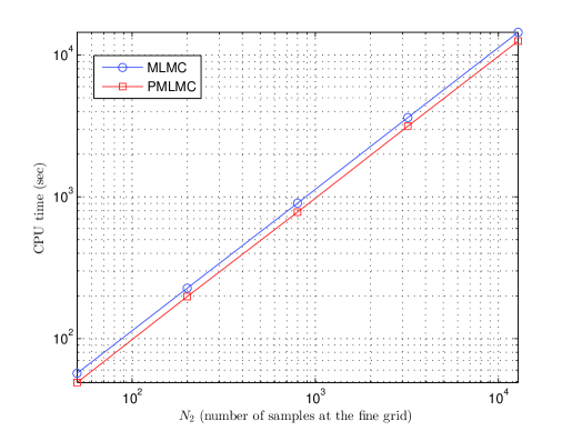
Figure 2. CPU time (sec) versus $N_{2}$ (number of samples at the fine grid) for MLMC and PMLMC methods in 1D corresponding to Left of Table 1.

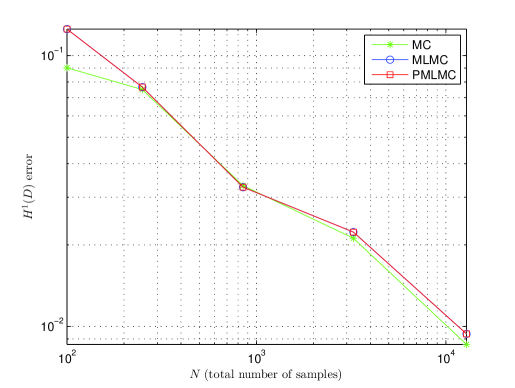
Figure 3. $H^{1}(D)$ error versus $N$ (total number of samples) for MC, MLMC and PMLMC methods in 1D corresponding to Right of Table 1. The number of samples at the fine grid is fixed as $N_{2}=50$ for MLMC and PMLMC methods.

4.2. Results in 2D

We make eigenvalues in 2D from the tensor products of those in 1D, see Cliffe et al. [18] for details. We re-order eigenvalues in magnitude and truncate them up to $1000$ modes in the rectangular grid of size $1/128$.

We use the triangular mesh to compute approximations. The coarse grid is generated by DistMesh [42] with a mesh size $h=0.0442$. The fine mesh is made from the coarse grid using the mid point rule, and has a mesh size $h=0.0221$. The fine and coarse mesh grids form a hierarchical mesh system and make it possible to reduce the error by decreasing the unmatched node points between coarse and fine grids. Numbers of elements and nodes are $2934$, $1262$ at the coarse grid and $9576$, $4917$ at the fine grid, which means the fine grid has more than triple elements and nodes compared to those in the coarse grid.

We use the same machine with a Matlab code in 2D. It takes 6 days and 15 hours in CPU time for the calculation of $30000$ sample solutions. The PMLMC method speeds up at the fine grid by at least $18\%$ as tabulated in Left of Table 2 and depicted in Fig. 4. In Right of Table 2, we doubles numbers of samples at the fine grid while quadruples those at the coarse grid. We illustrate the results in Fig. 5. The main reason to increase $N_{2}$ is due to the slow convergence rate. We expect that we can fix $N_{2}$ when the mesh size is small enough as in the case of 1D.

Table 2. In Left, CPU time (sec) versus $N_{2}$ (number of samples at the fine grid) for MLMC and PMLMC methods in 2D. In Right, $H^{1}(D)$ error versus $N$ (total number of samples) for MC, MLMC and PMLMC methods in 2D. $N_{2}$ are $50,100,200,400,800$ for MLMC and PMLMC methods.

CPU Time (sec)
$N_{2}$	MLMC	PMLMC
50	1179	957
200	4728	3838
800	18911	15351
3200	75644	61405
12800	302577	245615

$H^{1}(D)$ error
$N$	MC	MLMC	PMLMC
100	$6.7379\times 10^{-2}$	$9.1351\times 10^{-2}$	$9.1353\times 10^{-2}$
300	$5.5589\times 10^{-2}$	$6.2854\times 10^{-2}$	$6.2687\times 10^{-2}$
1000	$2.4383\times 10^{-2}$	$3.7902\times 10^{-2}$	$3.7713\times 10^{-2}$
3600	$1.0850\times 10^{-2}$	$3.0330\times 10^{-2}$	$3.0255\times 10^{-2}$
13600	$5.2386\times 10^{-3}$	$2.9398\times 10^{-2}$	$2.9226\times 10^{-2}$

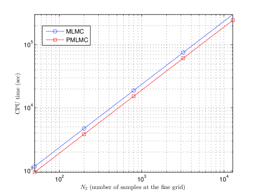
Figure 4. CPU time (sec) versus $N_{2}$ (number of samples at the fine grid) for MLMC and PMLMC methods in 2D corresponding to Left of Table 2.

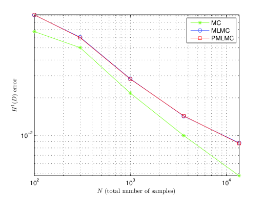
Figure 5. $H^{1}(D)$ error versus $N$ (total number of samples) for MC, MLMC and PMLMC methods in 2D corresponding to Right of Table 2. $N_{2}$ are $50,100,200,400,800$ for MLMC and PMLMC methods.

4.3. Cost Savings

For comparison of CPU time, we tabulate CPU times for MC, MLMC and PMLMC methods in Table 3. We illustrate the results in Fig. 6 and Fig. 7 for 1D and 2D, respectively. In 1D, the computational cost savings by the PMLMC method are constant, since the projection occurs only $50$ times.

In the fine grid, the PMLMC method spends almost same time as the MC method does, while the MLMC method does 14 % in 1D and 20 % in 2D more time than the MC method does, as tabulated in Left of Table 1 and Table 2 for 1D and 2D, respectively. We can say that the PMLMC method saves the computational cost further than the MLMC method. This is due to the solution procedure for the MLMC method in the coarse grid. To the contrary, the PMLMC method uses the projection, a cheaper procedure compared to the MLMC method in the view of cost savings.

Table 3. CPU time (sec) versus $N$ (total number of samples) for MC, MLMC and PMLMC methods in 1D (Left) and 2D (Right). The number of samples at the fine grid is fixed as $N_{2}=50$ for MLMC and PMLMC methods.

CPU Time (sec) in 1D
$N$	MC	MLMC	PMLMC
100	$99$	$68$	$60$
250	$246$	$100$	$93$
850	$837$	$227$	$218$
3250	$3201$	$734$	$726$
12850	$12729$	$3103$	$3091$

CPU Time (sec) in 2D
$N$	MC	MLMC	PMLMC
100	$1918$	$1409$	$1188$
300	$5754$	$3263$	$2825$
1000	$19187$	$8425$	$7508$
3600	$68995$	$24100$	$22243$
13600	$262352$	$77108$	$73220$

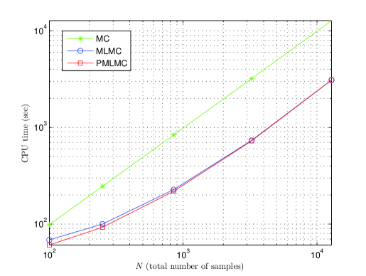
Figure 6. CPU time (sec) versus $N$ (total number of samples) for MC, MLMC and PMLMC methods in 1D corresponding to Left of Table 3. The number of samples at the fine grid is fixed as $N_{2}=50$.

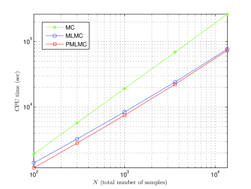
Figure 7. CPU time (sec) versus $N$ (total number of samples) for MC, MLMC and PMLMC methods in 2D corresponding to Right of Table 3. $N_{2}$ are $50,100,200,400,800$ for MLMC and PMLMC methods.

5. Conclusion

From the error estimations in Section 3, we confirm that the order of convergence of the MC method is $1/2$ which means that we need quadruple samples to decrease the error in half in the numerical simulation. MLMC and PMLMC methods are faster than the MC method and show the same order of convergence $1/2$. When the most computation occurs at the coarse grid, the computational cost due to the increase of samples does not increase, rather decreases proportional to the ratio of the number of samples at the coarse grid to that at the fine grid. In the PMLMC method, we use the projection from the fine grid to the coarse grid to replace the approximation at the coarse grid in the MLMC method, which results in the reduction of the computational cost further than the MLMC method.

The PMLMC method upgrades values at mid points of edges in the coarse grid when we use a hierarchical grid structure under mid point refinement scheme. This means that we can use small number of samples during the correction procedure in the fine grid, since the main structure of the mean value is estimated at the coarse grid by illustration of convergence of error in Fig. 3 and Fig. 5. Non-conforming finite element methods can be used for the PMLMC method since the PMLMC method does not require the inclusion of two consecutive approximate spaces.

The variance analysis and optimal number of samples with illustrations of them through numerical simulations in 1D and 2D are shown for the completeness of the paper. In the near future, we would present the results on MLMC and PMLMC methods combined with conforming and non-conforming finite elements applied to the Helmholtz equation with a random coefficient and wave equation with a white noise.

References

• [1] Abdulle, A., Barth, A., Schwab, C.: Multilevel Monte Carlo methods for stochastic elliptic multiscale PDEs. Multiscale Model. Simul. 11(4), 1033–1070 (2013)
• [2] Almroth, B.O., Stern, P., Brogan, F.A.: Automatic choice of global shape functions in structural analysis. AIAA J. 16, 525–528 (1978)
• [3] Arfken, G.: Mathematical Methods for Physicists, 3rd edn. Academic Press (1985)
• [4] Babuška, I., Aziz, A.K.: On the angle condition in the finite element method. SIAM J. Numer. Anal. 13, 214–226 (1976)
• [5] Babuška, I., Nobile, F., Tempone, R.: A stochastic collocation method for elliptic partial differential equations with random input data. SIAM J. Numer. Anal. 45(3), 1005–1034 (2007)
• [6] Babuška, I., Nobile, F., Tempone, R.: A stochastic collocation method for elliptic partial differential equations with random input data. SIAM Rev. 52(2), 317–355 (2010)
• [7] Babuška, I., Tempone, R., Zouraris, G.E.: Galerkin finite element approximations of stochastic elliptic partial differential equations. SIAM J. Numer. Anal. 42(2), 800–825 (2004)
• [8] Babuška, I., Tempone, R., Zouraris, G.E.: Solving elliptic boundary value problems with uncertain coefficients by the finite element method: the stochastic formulation. Comput. Methods Appl. Mech. Engrg. 194, 1251–1294 (2005)
• [9] Balmes, E.: Parametric families of reduced finite element models: theory and applications. Mech. Syst. Signal. Process. 10(4), 381–394 (1996)
• [10] Barrault, M., Maday, Y., Nguyen, N.C., Patera, A.T.: An ‘empirical interpolation’ method: application to efficient reduced basis discretization of partial differential equations. C. R. Math. Acad. Sci. Paris 339, 667–672 (2004)
• [11] Barrett, A., Reddien, G.: On the reduced basis method. Z. Angew. Math. Mech. 75(7), 543–549 (1995)
• [12] Barth, A., Lang, A., Schwab, C.: Multilevel Monte Carlo method for parabolic stochastic partial differential equations. BIT Numer. Math. 53, 3–27 (2013)
• [13] Barth, A., Schwab, C., Zollinger, N.: Multi-level Monte Carlo finite element method for elliptic PDEs with stochastic coefficients. Numer. Math. 119, 123–161 (2011)
• [14] Çinlar, E.: Probability and Stochastics, vol. XIV. Springer (2011)
• [15] Charrier, J., Scheichl, R., Teckentrup, A.L.: Finite element error analysis of elliptic PDEs with random coefficients and its application to multilevel Monte Carlo methods. SIAM J. Numer. Anal. 51(1), 322–352 (2013)
• [16] Ciarlet, P.G.: The Finite Element Method for Elliptic Problems. North-Holland, Amsterdam (1978)
• [17] Clenshaw, C.W., Curtis, A.R.: A method for numerical integration on an automatic computer. Numer. Math. 2, 197–205 (1960)
• [18] Cliffe, K.A., Giles, M.B., Scheichl, R., Teckentrup, A.L.: Multilevel Monte Carlo methods and applications to elliptic PDEs with random coefficients. Comput. Visual. Sci. 14, 3–15 (2011)
• [19] Eiermann, M., Ernst, O.G., Ullmann, E.: Computational aspects of the stochastic finite element method. Comput. Vis. Sci. 10, 3–15 (2007)
• [20] Frauenfelder, P., Schwab, C., Todor, R.A.: Finite elements for elliptic problems with stochastic coefficients. Comput. Methods Appl. Mech. Engrg. 194, 205–228 (2005)
• [21] Ghanem, R., Dham, S.: Stochastic finite element analysis for multiphase flow in heterogeneous porous media. Transport Porous Med. 32, 239–262 (1998)
• [22] Ghanem, R.G., Spanos, P.D.: Stochastic Finite Elements: A Spectral Approach. Springer-Verlag (1991)
• [23] Giles, M.B.: Multilevel Monte Carlo path simulation. Oper. Res. 56(3), 607–617 (2008)
• [24] Giles, M.B., Szpruch, L.: Antithetic multilevel Monte Carlo estimation for multi-dimensional SDEs without Lévy area simulation. Ann. Appl. Probab. 24(4), 1585–1620 (2014)
• [25] Glasserman, P.: Monte Carlo Methods in Financial Engineering, Applications of Mathematics, vol. 53. Springer (2003)
• [26] Gunzburger, M.D., Webster, C.G., Zhang, G.: Stochastic finite element methods for partial differential equations with random input data. Acta Numer. 23, 521–650 (2014)
• [27] Hamption, J., Doostan, A.: Compressive sampling of polynomial chaos expansions: convergence analysis and sampling strategies (2014). ArXiv:1408.4157v3 [math.PR]
• [28] Heinrich, S.: Multilevel Monte Carlo Methods, Lecture Notes in Comput. Sci., vol. 2179, pp. 58–67. Springer, Berlin (2001)
• [29] Hoeksema, R.J., Kitanidis, P.K.: Analysis of the spatial structure of properties of selected aquifers. Water Resour. Res. 21, 536–572 (1985)
• [30] Hou, T.Y., Liu, P.: A heterogeneous stochastic fem framework for elliptic PDEs. J. Comput. Phys. 281, 942–969 (2015)
• [31] Jamet, P.: Estimations d’erreur pour des elements finis droits presque degeneres. R.A.I.R.O. Anal. Numer. 10, 43–61 (1976)
• [32] Khoromskij, B.N., Schwab, C.: Tensor-structured galerkin approximation of parametric and stochastic elliptic PDEs. SIAM J. Sci. Comput. 33(1), 364–385 (2011)
• [33] Loève, M.: Probability Theory. I, Grad. Texts in Math., vol. 45, 4th edn. Springer-Verlag, New York (1977)
• [34] Loève, M.: Probability Theory. II, Grad. Texts in Math., vol. 46, 4th edn. Springer-Verlag, New York (1978)
• [35] Maday, Y., Patera, A.T., Turinici, G.: A priori convergence theory for reduced-basis approximations of single-parametric elliptic partial differential equations. J. Sci. Comput. 17, 437–446 (2002)
• [36] MATLAB: version 8.0.0.783 (R2012b). The MathWorks Inc., Natick, Massachusetts (2012)
• [37] Matthies, H.G., Keese, A.: Galerkin methods for linear and nonlinear elliptic stochastic partial differential equations. Comput. Methods Appl. Mech. Engrg. 194, 1295–1295 (2005)
• [38] Migliorati, G., Nobile, F., von Schwerin, E., Tempone, R.: Approximation of quantities of interest in stochastic PDEs by the random discrete ${L}^{2}$ projection on polynomial spaces. SIAM J. Sci. Comput. 35(3), A1440–A1460 (2013)
• [39] Migliorati, G., Nobile, F., von Schwerin, E., Tempone, R.: Analysis of discrete ${L}^{2}$ projection on polynomial spaces with random evaluations. Found. Comput. Math. 14, 419–456 (2014)
• [40] Nobile, F., Tempone, R., Webster, C.G.: An anisotropic sparse grid stochastic collocation method for partial differential equations with random input data. SIAM J. Numer. Anal. 46(5), 2411–2442 (2008)
• [41] Nobile, F., Tempone, R., Webster, C.G.: A sparse grid stochastic collocation method for partial differential equations with random input data. SIAM J. Numer. Anal. 46(5), 2309–2345 (2008)
• [42] Persson, P.O., Strang, G.: A simple mesh generator in matlab. SIAM Rev. 46(2), 329–345 (2004)
• [43] Pomplun, J., Schmidt, F.: Accelerated a posteriori error estimation for the reduced basis method with application to 3d electromagnetic scattering problems. SIAM J. Sci. Comput. 32(2), 498–520 (2010)
• [44] Prato, G.D., Zabczyk, J.: Stochastic equations in infinite dimensions, Encyclopedia of Mathematics and its Applications, vol. 44. Cambridge University Press (1992)
• [45] Smolyak, S.A.: Quadrature and interpolation formulas for tensor products of certain classes of functions. Dokl. Akad. Nauk SSSR 4, 240–243 (1963)
• [46] Stefanou, G.: The stochastic finite element method: Past, present and future. Comput. Methods Appl. Mech. Engrg. 198, 1031–1051 (2009)
• [47] Teckentrup, A.L., Jantsch, P., Webster, C.G., Gunzburger, M.: A multilevel stochastic collocation method for partial differential equations with random input data (2014). ArXiv:1404.2647v2 [math.NA]
• [48] Xiu, D.: Numerical methods for stochastic computations: a spectral method approach. Princeton University Press (2010)
• [49] Xiu, D., Hesthaven, J.S.: High-order collocation methods for differential equations with random inputs. SIAM J. Sci. Comput. 27(3), 1118–1139 (2005)
• [50] Xiu, D., Karniadakis, G.E.: The wiener-askey polynomial chaos for stochastic differential equations. SIAM J. Sci. Comput. 24, 619–644 (2002)
• [51] Xiu, D., Karniadakis, G.E.: Modeling uncertainty in flow simulations via generalized polynomial chaos. J. Comput. Phys. 187, 137–167 (2003)
• [52] Zlámal, M.: On the finite element method. Numer. Math. 12, 394–409 (1968)