Long-range order and pinning of charge-density waves in competition with superconductivity

Abstract

Recent experiments show that charge-density wave correlations are prevalent in underdoped cuprate superconductors. The correlations are short-ranged at weak magnetic fields but their intensity and spatial extent increase rapidly at low temperatures beyond a crossover field. Here we consider the possibility of long-range charge-density wave order in a model of a layered system where such order competes with superconductivity. We show that in the clean limit, low-temperature long-range order is stabilized by arbitrarily weak magnetic fields. This apparent discrepancy with the experiments is resolved by the presence of disorder. Like the field, disorder nucleates halos of charge-density wave, but unlike the former it also disrupts inter-halo coherence, leading to a correlation length that is always finite. Our results are compatible with various experimental trends, including the onset of longer range correlations induced by inter-layer coupling above a characteristic field scale.

I Introduction

The pseudogap state of the cuprate high-temperature superconductors (HTSCs) harbors various fluctuating electronic orders.intertwined In particular, recent nuclear magnetic resonance (NMR) NMR-nature ; NMR-nature-comm ; NMR-arxiv and x-ray scattering Ghiringhelli ; Chang ; Achkar1 ; Blackburn13 ; Achkar2 ; Comin1 ; daSilva ; Le-Tacon ; Hucker ; Blanco-Canosa ; Tabis ; Croft ; SilvaNeto ; Comin3 ; Comin-symmetry ; Gerber measurements have found evidence of charge-density wave (CDW) fluctuations across this family of materials. The observed strength of the CDW fluctuations is anti-correlated with superconductivity (SC) in the sense that the intensity of the CDW scattering peak grows as the temperature is reduced towards the superconducting transition temperature, $T_{c}$, and then decreases or saturates upon entering the SC phase. In addition, the CDW signal is enhanced when a magnetic field is used to quench SC, while the effect of a magnetic field above $T_{c}$ is negligible. Finally, optical excitation of apical oxygen vibrations promotes transient superconducting signatures in YBa₂Cu₃O_6+x,Hu ; Kaiser resembling similar results in La_1.675Eu_0.2Sr_0.125CuO₄,Fausti where they were conjectured to be a consequence of the melting of charge stripe order.Forst

Motivated by these findings, Hayward et al.  Hayward1 ; Hayward2 proposed a phenomenological non-linear sigma model (NLSM), which formulates the competition between fluctuating SC and CDW order parameters. Similar models emerge also from more microscopic considerations.Metlitski ; Efetov ; Meier ; Einenkel-vortex Using Monte-Carlo simulations, Hayward et al.  calculated the temperature dependence of the x-ray structure factor in the absence of a magnetic field and showed that it exhibits a maximum slightly above the Berezinskii-Kosterlitz-Thouless temperature, $T_{BKT}$, of their two-dimensional model. The fact that a similar peak appears in zero-field x-ray scattering from YBa₂Cu₃O_6+xGhiringhelli ; Chang ; Achkar1 and La_2-xSr_xCuO₄,Croft was taken as an encouraging sign that the NLSM is able to capture salient features of the data. The situation, however, is more complicated and the structure factor of HgBa₂CuO_4+δTabis shows no such peak. It is therefore interesting to explore the extent to which one can reproduce and understand the various trends revealed by experiments from the perspective of a simple model of competing orders. In particular, we would like to ask this question with regard to the transition from short-range correlations at low magnetic fields to longer range order at high fields, as detected by NMRNMR-nature-comm , ultrasoundultrasound and most recently x-ray scatteringGerber measurements.

To this end we incorporate into the NLSM of Ref. Hayward1, three additional ingredients that are important for comparison with experiments, namely, inter-layer couplings, a magnetic field and random pinning potentials. We analyze their effects on CDW signatures and ordering tendencies via a large-$N$ approximation, previously used by us to study the consequences of thermally excited vortices in the NLSM.nlsm-vortex Averages over disorder are calculated with the replica method, and emphasis is put on the low-temperature SC phase where the effects of the additional factors are significant. We also present complementary results of Monte-Carlo simulations, which we use to study the model beyond the limits of our analytical approach.

We show that in a clean system, without a magnetic field, the competition with SC establishes a threshold inter-layer coupling for the stabilization of long-range CDW order. On the other hand, in the presence of a magnetic field, any small inter-layer coupling suffices to induce long-range order between the CDW regions which nucleate around the cores of the Abrikosov vortices. These results are also reflected in the low-temperature CDW structure factor of weakly coupled layers. While it vanishes linearly with decreasing temperature in the field-free system, it diverges when a field is present. Both behaviors are inconsistent with the x-ray data.

In contrast, qualitative agreement with the experimental phenomenology is obtained when the effects of a random pinning potential are taken into account. Since favorable disorder configurations nucleate CDW regions that survive the competition with SC down to zero temperature, the structure factor attains a non-zero finite value in this limit. This value grows with magnetic field, which adds vortices as CDW nucleation centers, but true long-range phase order between the CDW regions, predicted by mean-field theory, is avoided due to the Imry-Ma argument.Imry-Ma Nevertheless, we find that as the field is increased through the failed mean-field transition, the correlation length is significantly enhanced by the effects of inter-layer couplings. At higher temperatures the structure factor exhibits a maximum close to $T_{c}$, which is washed away by both magnetic field and stronger disorder strength, while at even higher temperatures it becomes magnetic field-independent. The crossover field changes little until somewhat below $T_{c}$, where it diverges. However, the increase in the correlation length across it diminishes with temperature. The reflection of these trends in experiments indicates that both order competition and disorder are crucial elements in understanding the physics of underdoped cuprates.

In the next section we introduce the model and lay out our findings while moving up in complexity from the single clean layer to a disordered system of coupled layers. The technical derivations of the results are relegated to the appendices. In the final section we discuss our work in view of experiments done in underdoped cuprates.

II Model and Results

II.1 The clean, single layer NLSM

We begin with the model considered by Hayward et al. ,Hayward1 for a real 6-dimensional order parameter, equivalent to a complex SC field $\Psi=n_{1}+in_{2}$ and two complex CDW fields, $\Phi_{x}=n_{3}+in_{4}$ and $\Phi_{y}=n_{5}+in_{6}$. Here, for the sake of simplicity, we disregard quartic and anisotropic CDW terms, which appear in Ref. Hayward1, , and follow our previous strategynlsm-vortex of using a saddle-point approximation for the CDW fields, which is formally justified when their number is large. Thus, we analyze a system described by a complex SC field $\{\psi,\psi^{*}\}$, and $N-2$ real CDW fields $\{n_{\alpha}\}$, where $\alpha=1\dots N-2$, whose Hamiltonian is

$$H_{0}[\psi,n_{\alpha}] = \frac{1}{2}\rho_{s}\int d^{2}r\,\Big{\{}|(\bm{\nabla}+2ie{\bf A})\psi|^{2}$$ (1)

$$\qquad+\sum_{\alpha=1}^{N-2}\left[\lambda(\bm{\nabla}n_{\alpha})^{2}+gn_{\alpha}^{2}\right]\Big{\}},$$

where $\rho_{s}$ is the stiffness of the SC order, $\lambda\rho_{s}$ is the corresponding quantity for the CDW components, and $g\rho_{s}$ is the energy density penalty for CDW ordering. We assume that some type of order (SC or CDW) is always locally present, in the sense of its amplitude, but that the different order parameters compete, as expressed by the constraint

$$|\psi|^{2}+\sum_{\alpha=1}^{N-2}n_{\alpha}^{2}=1.$$ (2)

The free energy $F_{0}$ is given by

$$e^{-\beta F_{0}} = \int\mathcal{D}\psi^{*}\mathcal{D}\psi\mathcal{D}n\,\delta\left(|\psi|^{2}+\sum_{\alpha=1}^{N-2}n_{\alpha}^{2}-1\right)e^{-\beta H_{0}}$$ (3)

$$= \int\mathcal{D}\psi^{*}\mathcal{D}\psi\mathcal{D}n\mathcal{D}\bar{\sigma}\,e^{-\beta H_{0}}$$

$$\qquad\qquad\times e^{\frac{1}{2}\beta\rho_{s}\int d^{2}r\,i\bar{\sigma}\left(|\psi|^{2}+\sum_{\alpha}n_{\alpha}^{2}-1\right)},$$

where $\beta=1/T$ is the inverse temperature. In the limit $N\to\infty$ we integrate over $n_{\alpha}$ while assuming that the Lagrange multiplier field, $\bar{\sigma}$, attains its saddle-point configuration, $\bar{\sigma}=i\sigma$. Since we are focusing on signatures of the CDW deep inside the SC phase, $T\ll T_{BKT}$, we also assume that the SC fields $\psi,\psi^{*}$ take their saddle-point configurations. Within this approximationfn-Demler , the free energy of the clean layer is given by

$$\beta F_{0} = \frac{N-2}{2}{\rm Tr}\ln\left[\frac{1}{2}\beta\rho_{s}\left(-\lambda\nabla^{2}+g+\sigma\right)\right]$$

$$+\frac{1}{2}\beta\rho_{s}\int d^{2}r\left[|(\bm{\nabla}+2ie{\bf A})\psi|^{2}+\sigma\left(|\psi|^{2}-1\right)\right],$$

where the fields $\psi,\psi^{*}$ and $\sigma$ are determined by the coupled saddle-point equations

$$\frac{\delta\,\beta F_{0}}{\delta\psi^{*}({\bf r})}=\frac{1}{2}\beta\rho_{s}\left[-(\bm{\nabla}+2ie{\bf A})^{2}+\sigma\right]\psi=0,$$ (5)

and

$$\frac{\delta\,\beta F_{0}}{\delta\sigma({\bf r})} = \frac{N-2}{2}{\rm Tr}\left[\left(-\lambda\nabla^{2}+g+\sigma\right)^{-1}\delta_{\bf r}\right]$$ (6)

$$+\frac{1}{2}\beta\rho_{s}\left(|\psi|^{2}-1\right)=0,$$

with $\delta_{\bf r}({\bf r}^{\prime},{\bf r}^{\prime\prime})=\delta({\bf r}^{\prime}-{\bf r})\delta({\bf r}^{\prime\prime}-{\bf r})$.

We first consider the case of zero magnetic field, where the SC field assumes a uniform configuration, $\psi({\bf r})=\psi_{0}$, and $\sigma=0$. By substituting this solution in equation (6) we find that

$$|\psi_{0}|^{2}=1-\frac{T}{T_{MF}},$$ (7)

where the mean-field transition temperature is given by

$$\frac{\rho_{s}}{T_{MF}} = \frac{N-2}{\lambda}{\rm Tr}\left[\left(-\nabla^{2}+g/\lambda\right)^{-1}\delta_{{\bf r}}\right]$$ (8)

$$\simeq \frac{N-2}{4\pi\lambda}\ln\left(\frac{32\lambda}{ga^{2}}\right).$$

To obtain the last expression we regularized the theory by putting it on a square lattice of spacing $a$, and assumed $ga^{2}/\lambda\ll 1$. The CDW structure factor, is defined by

$$S({\bf q})=\frac{1}{L^{2}}\int d^{2}r\,d^{2}r^{\prime}\,e^{-i{\bf q}\cdot({\bf r}-{\bf r}^{\prime})}\braket{n_{\alpha}({\bf r})n_{\alpha}({\bf r}^{\prime})},$$ (9)

where ${\bf q}$ is measured from the ordering wavevector of $n_{\alpha}$, $L^{2}$ is the layer’s area, and $\braket{\cdots}$ denotes thermal averaging. We will concentrate on the peak value $S_{CDW}\equiv S({\bf q}=0)$, deferring the ${\bf q}$ dependence to Appendix A. Here, the uniformity of $\psi$ and $\sigma$ readily leads to the result

$$S_{CDW}=\frac{T}{g\rho_{s}},$$ (10)

which vanishes as $T\to 0$.

The situation changes upon applying a magnetic field, $B$. The solution of the saddle-point equations (5,6) is expected to take the form of an Abrikosov lattice of vortices, whose density is determined by the magnetic field. Far away from the vortex cores, $\sigma=0$ and $\psi=\psi_{0}$, just as in the zero field case. However, close to the center of each vortex, $\psi$ vanishes linearly with the distance from the vortex center, and $\sigma$ becomes negative. As a result, there is a trapped CDW mode inside each core, in addition to a continuum of scattering modes, which exists also without a magnetic field. Using a tight-binding approximation (see Appendix A) for these trapped modes in equation (6), we can estimate their contribution to $S_{CDW}$. The result depends on the order of limits. At a low but non-zero temperature, and $B\to 0$ (more precisely, when $t\sim ge^{-c_{1}\sqrt{g\phi_{0}/B}}\ll gT/\rho_{s}$), we find that

$$S_{CDW}=\frac{T}{g\rho_{s}}+A_{1}\left[1-\left(\frac{A_{2}}{\rho_{s}}+\frac{1}{T_{MF}}\right)T\right]\frac{B}{g^{2}\phi_{0}},$$ (11)

where $\phi_{0}=\pi\hbar c/e$ is the flux quantum. Here, and throughout the paper, we denote by $A_{i}$,$b_{i}$, and $c_{i}$ various numerical constants. In the other limit, of a finite magnetic field and $T\to 0$ (when $t\gg gT/\rho_{s}$), we obtain

$$S_{CDW}=A_{3}\frac{T}{t\rho_{s}}\frac{B}{g\phi_{0}}e^{c_{2}(t/g)\rho_{s}(1/T-1/T_{MF})}.$$ (12)

Therefore, the structure factor diverges at low temperatures in the presence of a magnetic field.

In order to go beyond our mean-field results, we performed Monte-Carlo (MC) simulations of the NLSM, incorporating the effects of a uniform magnetic field, as appropriate for an extreme type-II superconductor. We used standard Metropolis updating to study systems on a square $L\times L$ lattice, with $L$ ranging from 32 to 200 sites, and cylindrical boundary conditions. We present here MC results for the experimentally relevant case, $N=6$, and additionally set $\lambda=1$ and $ga^{2}=0.3$. For these parameters, $T_{BKT}/\rho_{s}=0.345$. To facilitate comparison with the results of Ref. Hayward1, , we present in Fig. 1a the structure factor $S_{\Phi_{x}}/a^{2}=2S_{CDW}/a^{2}$ as a function of $T$ in a clean layer with and without a magnetic field. For $B=0$, $S_{\Phi_{x}}$ vanishes linearly as $T$ approaches zero in agreement with equation (10), but diverges at low $T$ for finite $B>0$, as in equation (12). Our results are generally independent of the system size, except for the $B>0,T\to 0$ limit, where the diverging $S_{\Phi_{x}}$ increases with $L$.

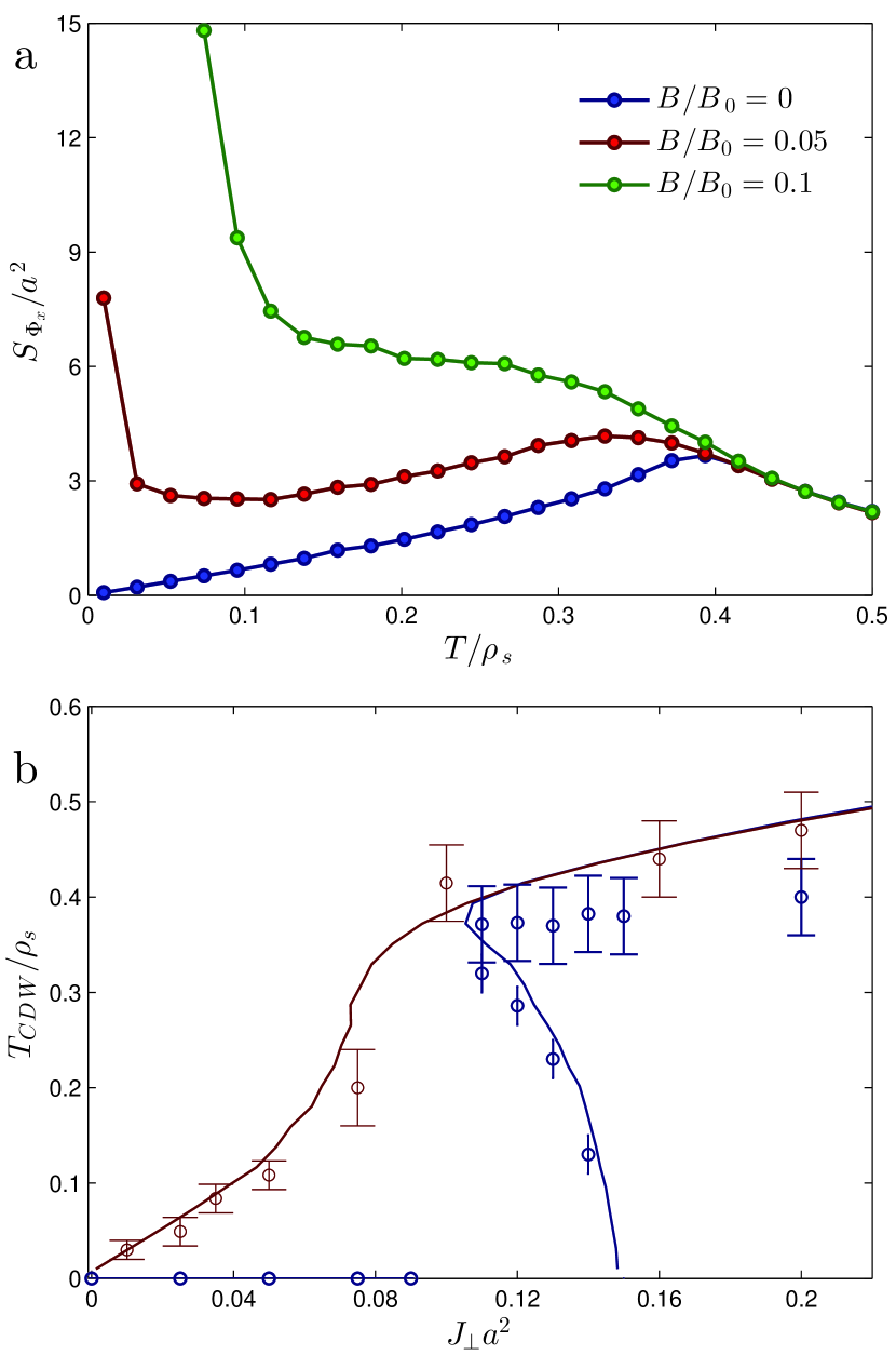
Figure 1: Onset of long-range CDW order in the clean system. (a) The structure factor of a clean $48\times 48$ layer with $\lambda=1$ and $ga^{2}=0.3$, as function of $T$ for three values of $B/B_{0}$, where $B_{0}=\phi_{0}/2\pi a^{2}$. (b) The CDW ordering temperature, estimated from a $32\times 32\times 8$ multi-layer with the same parameters, at $B=0$ and $B=0.05B_{0}$. The lines depict the solution of the interlayer mean-field condition, equation (14).

II.2 Clean coupled layers

Next, we would like to ask whether a weak interlayer CDW coupling is sufficient to stabilize long-range CDW order. First, let us note that the diverging SC susceptibility of each layer at $T_{BKT}$ implies that any weak interlayer Josephson coupling of the form $-\rho_{s}J_{SC}\int d^{2}r\sum_{i}\left[\psi^{*}_{i}\psi_{i+1}+{\rm H.c.}\right]$, where $i$ is the layer index, induces long-range SC order. However, for weak $J_{SC}$ the SC transition at $T_{c}=T_{BKT}\left[1+b_{1}/\ln^{2}(b_{2}\,g/J_{SC})\right]$, (see Appendix B), has only a small effect on $|\psi|$ and thus on the amplitude and ordering tendencies of $n$. Consequently, we concentrate on the following multi-layer Hamiltonian

$$H=\sum_{i}H_{0}[\psi_{i},n_{\alpha,i}]-\rho_{s}J_{\perp}\int d^{2}r\sum_{\alpha,i}n_{\alpha,i}n_{\alpha,i+1}.$$ (13)

CDWs on different layers are coupled capacitively. The small amplitude of the charge modulation associated with the CDW, and its $d$-wave natureComin-symmetry ; Fujita-symmetry imply a weak CDW coupling with a complicated real-space structure. We defer the study of the consequences of such structure to a future publication and instead treat here the simplest model interaction, as expressed in Eq. (13). In the following we choose $J_{\perp}>0$, although a purely repulsive interaction corresponds to $J_{\perp}<0$. However, the two cases are related by the transformation $n_{\alpha,i}\rightarrow(-1)^{i}n_{\alpha,i}$, which reverses the sign of $J_{\perp}$ but leaves $H_{0}$ unchanged. Consequently, our conclusions regarding the presence of long-range CDW order hold for both attractive and repulsive interactions, with the only difference being a change in the $c$-axis ordering wave-vector from 0 to $\pi/a$.

To estimate the effect of $J_{\perp}$ we use the interlayer mean-field approximationinterMF ; striped (see Appendix B) which in the absence of a field yields the following condition for the putative CDW ordering transition

$$1=2\rho_{s}J_{\perp}\chi(T_{CDW}),$$ (14)

expressed in terms of the in-plane CDW susceptibility $\chi(T)$. For a clean system $\chi(T)=S_{CDW}(T)/T$ and equation (10) implies that condition (14) can be fulfilled only if $J_{\perp}\geq g/2$. When this happens uniform CDW order is established, and the interlayer coupling term in equation (13) leads to the effective modification $g\rightarrow g-2J_{\perp}\langle n_{\alpha}\rangle^{2}/\langle n_{\alpha}^{2}\rangle$. Hence, for $J_{\perp}\geq g/2$ and $T\rightarrow 0$ the effective $g$ turns negative, SC disappears and the system becomes purely CDW ordered.

In the presence of a weak magnetic field and at low temperatures, the right hand side of the mean-field condition (14) acquires an additional factor which scales as $B/g\phi_{0}$. However, more important for establishing the qualitative difference compared to the field-free case is the low-$T$ divergence of $S_{CDW}$, equation (12). This means that even for $J_{\perp}\rightarrow 0$, long-range order between the CDW regions around the vortex cores does set in at $T_{CDW}=c_{2}t\rho_{s}/[g\ln(c_{3}t/J_{\perp})]$, and coexists with long-range SC order.

Fig. 1b depicts $T_{CDW}$ obtained from the onset temperature of the order parameter $\sum_{\alpha}\langle\sum_{i}\int d^{2}r\,n_{\alpha,i}\rangle^{2}$ in a clean $32\times 32\times 8$ layered system, as a function of the interlayer CDW coupling $J_{\perp}a^{2}$. As expected from the above mean-field considerations, we find a transition for $J_{\perp}>g/2$ and $B=0$, and down to the lowest accessible values of $J_{\perp}$ when $B>0$. In addition, however, for $J_{\perp}$ slightly below $g/2$ and $B=0$, we observe a transition to an ordered phase which vanishes at a lower critical temperature. This behavior can be traced to a maximum, $\chi_{\rm max}$, in $\chi=S_{CDW}/T$, which gives two solutions to equation (14) in the range $1/2\rho_{s}\chi_{\rm max}<J_{\perp}<g/2$.

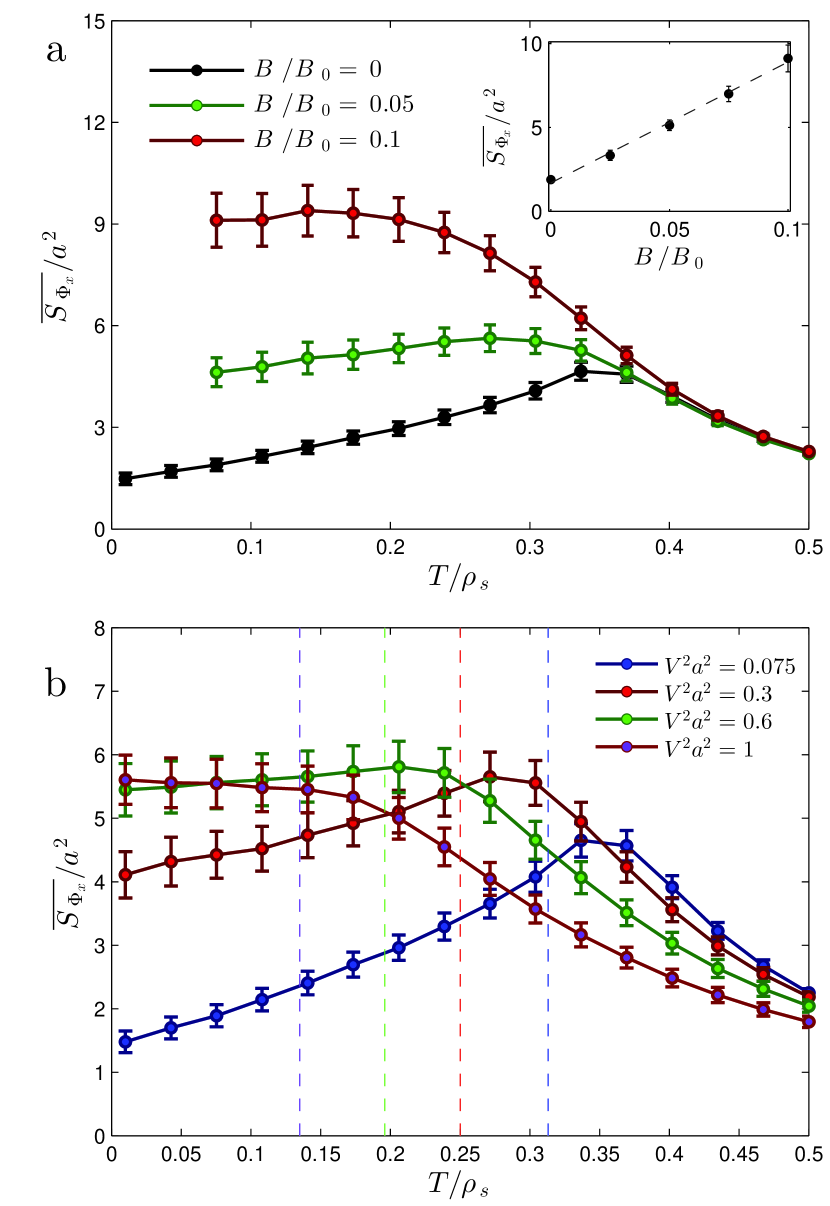
Figure 2: The structure factor of a disordered layer. (a) $\overline{S_{\Phi_{x}}}/a^{2}$ of a disordered $48\times 48$ layer with $\lambda=1$, $ga^{2}=0.3$ and $V^{2}a^{2}=0.075$. The inset depicts $\overline{S_{\Phi_{x}}}/a^{2}$ as function of $B$, for $T=0.075\rho_{s}$. (b) $\overline{S_{\Phi_{x}}}/a^{2}$ of the same layer at $B=0$, for various levels of disorder strength. The vertical lines depict $T_{BKT}$ of each system, as deduced from the calculated superconducting phase stiffness.

Figure 3: Crossover to longer-range CDW order in the disordered system. (a) The crossover line from short-range to longer-range CDW order, as deduced from the interlayer mean-field approximation for a $64\times 64\times 16$ disordered system with $\lambda=1$, $ga^{2}=0.3$, $V^{2}a^{2}=0.075$ and $J_{\perp}a^{2}=0.1$. The red dots depict the onset of enhanced field and temperature dependence of the in-plane correlation length. (b) The structure factor, averaged over 50 disorder realizations, as function of temperature. The inset show the CDW susceptibility of a single layer, used to derive the mean-field crossover line. (c) Magnetic field dependence of the structure factor. (d) Magnetic field dependence of the in-plane correlation length.

II.3 Disordered single layer

The fact that the behavior of the clean system, detailed above, is at odds with experiments motivates us to consider the effects of a random potential, which pins the CDW. We begin with the Hamiltonian of a single disordered layer

$$H_{0}[\psi,n_{\alpha};V_{\alpha}]=H_{0}[\psi,n_{\alpha}]-\rho_{s}\int d^{2}r\,\sum_{\alpha}V_{\alpha}n_{\alpha},$$ (15)

where $V_{\alpha}$ are independent random Gaussian fields satisfying $\overline{V_{\alpha}}=0$ and $\overline{V_{\alpha}({\bf r})V_{\beta}({\bf r}^{\prime})}=V^{2}\delta_{\alpha\beta}\delta({\bf r}-{\bf r}^{\prime})$, with the overline signifying disorder averaging.

Applying the replica method to the $N\to\infty$ limit large-n-replica ; large-n-replica2 we adapt the saddle-point equations (5,6) to the weakly disordered case, and calculate the structure factor $\overline{S_{CDW}}$, averaged over realizations of the pinning field. In the zero field case we find (see Appendix C)

$$\overline{S_{CDW}}=\frac{T}{g\rho_{s}}+\frac{V^{2}}{g^{2}},$$ (16)

which decreases linearly to a finite value as the temperature is reduced to zero. Such behavior reflects the fact that due to the random field certain regions assume local CDW order even at $T=0$. When the system is subject to a magnetic field, superconductivity is suppressed inside the vortex cores, around which CDW halos are formed. As a result, a larger fraction of the system’s area supports pinned local CDW order, and $\overline{S_{CDW}}$ increases. As long as $t\ll\max(gT/\rho_{s},\sqrt{gV^{2}})$ we find that (see Appendix C)

$$\!\!\!\!\!\!\!\!\!\!\!\overline{S_{CDW}}\! = \!\frac{T}{g\rho_{s}}+\frac{V^{2}}{g^{2}}$$ (17)

$$+ \!A_{1}\!\left[1-\left(\frac{A_{2}}{\rho_{s}}+\frac{1}{T_{MF}}\right)T-A_{4}\frac{V^{2}}{g}\right]\!\frac{B}{g^{2}\phi_{0}}.$$

A similar functional form characterizes the $T\to 0$ spatially averaged Edwards-Anderson order parameter

$$q_{EA}=\frac{1}{L^{2}}\int d^{2}r\overline{\braket{n_{\alpha}({\bf r})}^{2}}=\frac{V^{2}}{4\pi\lambda g}+A_{5}\frac{B}{g\phi_{0}}.$$ (18)

Random-field models in the $N\to\infty$ limit do not exhibit a glass transitionlarge-n-replica , and $q_{EA}>0$ for all $T$.

In Fig. 2a we present results for $\overline{S_{\Phi_{x}}}$, averaged over 60 disorder realizations, for a layer with $V^{2}a^{2}=0.075$. The inset depicts its low-temperature $B$ dependence. In accordance with our analytical result, equation (17), $\overline{S_{\Phi_{x}}}$ assumes a finite value for $T,B\to 0$, and grows linearly with both $T$ and $B$. The error bars in our MC results, which grow with increasing $B$ and decreasing $T$, reflect the low convergence rates and sensitivity to initial conditions which arise in this limit. However, our MC simulations clearly show that $\overline{S_{\Phi_{x}}}$ does not diverge when $B>0$, even for temperatures below the range presented in the figure. In Fig. 2b we show $\overline{S_{\Phi_{x}}}/a^{2}$ of the same system at $B=0$ for various disorder strengths. The figure also depicts the BKT transition temperature for each system, as deduced from the calculated renormalized superconducting phase stiffness $\rho_{s}(T)$ and the BKT criterion $\rho_{s}(T_{BKT})=2T_{BKT}/\pi$. Our results clearly show that the peak in the structure factor, which occurs slightly above $T_{BKT}$, disappears with increasing disorder strength. At the same time the zero-temperature value of $\overline{S_{\Phi_{x}}}/a^{2}$ increases and approaches a limiting value as global superconducting order is suppressed by the disorder.

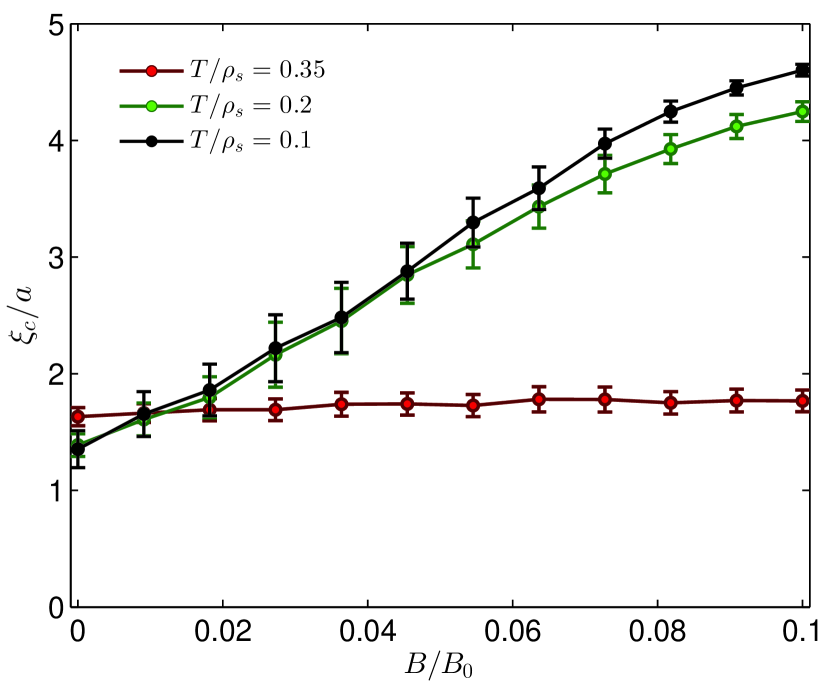
Figure 4: The inter-plane correlation length. The magnetic field dependence of $\xi_{c}$ for a $64\times 64\times 16$ disordered system with $\lambda=1$, $ga^{2}=0.3$, $V^{2}a^{2}=0.075$ and $J_{\perp}a^{2}=0.1$, averaged over 50 disorder realizations.

Figure 5: Temperature dependence of the correlation lengths. $\xi_{ab}$ and $\xi_{c}$ for a $64\times 64\times 16$ disordered system with $\lambda=1$, $ga^{2}=0.3$, $V^{2}a^{2}=0.075$ and $J_{\perp}a^{2}=0.1$, averaged over 50 disorder realizations.

II.4 Coupled disordered layers

Finally, consider the disordered version of the coupled-layer Hamiltonian (13), where each plane is described by $H_{0}[\psi,n_{\alpha};V]$, equation (15). While interlayer mean-field approximation predicts a CDW ordering transition at $T_{CDW}$, given by condition (14), the Imry-Ma argumentImry-Ma precludes long-range CDW order in a disordered system below four dimensions. Nevertheless, for weak disorder we expect the failed thermodynamic transition to leave its mark in the form of a crossover, which signifies the onset of enhanced CDW correlations within and between the planes.

To test this prediction, we start by evaluating the mean-field transition temperature from condition (14). We do so by calculating the disordered-averaged CDW susceptibility, $\overline{\chi}$, for a layer with $\lambda=1$, $ga^{2}=0.3$ and $Va^{2}=0.075$, which exhibits an x-ray structure factor with a similar temperature dependence to the one measured at low fields in YBa₂Cu₃O_6+x,Chang (see Fig. 2a). The results, presented in the inset of Fig. 3b, show that $\overline{\chi}$ is approximately constant at low $T$ and grows linearly with $B$ from $1/\rho_{s}g$, in accord with our large-$N$ analysis (see Appendix C). When combined with equation (14) this implies, for $J_{\perp}<\rho_{s}g/2$, a mean-field transition that occurs at a critical field which is constant over a wide temperature range and then increases rapidly. Such behavior, depicted in Fig. 3a for a system with $J_{\perp}a^{2}=0.1$, resembles that of the transition line into a long-range CDW phase, as deduced from ultrasound measurements.ultrasound

Next, let us inquire what features of the mean-field transition survive the effects of fluctuations. Fig. 3b depicts the temperature dependence of the structure factor (now defined by the average of $\langle n_{\alpha}({\bf r})n_{\alpha}({\bf r}^{\prime})\rangle$ over the three-dimensional system). While the qualitative features follow the ones displayed by the two-dimensional layer, the coupled layers exhibit, at low $T$, a rapidly increasing $\overline{S_{\Phi_{x}}}$ beyond a characteristic field scale, (see Fig. 3c). Another relevant signature is displayed by the in-plane correlation length, $\xi_{ab}$, defined by the inverse half-width at half maximum of $\overline{S_{\Phi_{x}}}({\bf q})$. Its field dependence, shown in Fig. 3d, exhibits an inflection point across the same magnetic field scale. Recent x-ray measurementsGerber have found a similar behavior in YBa₂Cu₃O_6+xat a range of magnetic fields that is comparable to ours if one identifies the short-distance scale, $a$, of the NLSM with 2-3 Cu-Cu spacings. Using also the temperature dependence of $\xi_{ab}$ and the corresponding data for the inter-plane correlation length, $\xi_{c}$, (see Figs. 4 and 5) we can map out the crossover field in the $B-T$ plane, and find that it follows the mean-field transition line. Hence, the following picture emerges: At weak magnetic fields the CDW correlations are short-ranged and largely confined to the planes. However, as the field increases at low temperatures, it combines with the inter-plane coupling to induce a crossover to more extended three-dimensional correlations. This crossover becomes sharper with diminishing disorder.

III Discussion

We have shown that competition between CDW and SC orders in the presence of disorder, can account for many of the trends observed in x-ray scattering experiments. Specifically, nucleation of CDW at regions of strong attractive disorder makes $S_{CDW}$ attain a finite value at $T=0$, even for $B=0$.Ghiringhelli ; Tabis ; Croft This value increases linearly with low $B$,Chang due to pinned CDW around vortex cores, as seen in scanning-tunneling experimentsHoffman ; Hamidian ; Machida . At higher temperatures and for weak disorder both our simulations and experiments on YBa₂Cu₃O_6+xChang and La_2-xSr_xCuO₄Croft exhibit a maximum in $S_{CDW}$ close to $T_{c}$, which disappears with increasing $B$, while there is practically no $B$ dependence beyond this temperature.Chang We find that the peak is also washed away with increasing disorder, a fact which may explain its absence in HgBa₂CuO_4+δ.Tabis . We note, however, that the predicted linear low-$T$ dependence for $B=0$, (see Fig. 3), is reflected in someCroft , but not all x-ray data.Chang Another discrepancy exists with Ref. Achkar2, , where $S_{CDW}$ was found to decrease upon increasing the amount of oxygen disorder.

Our results also demonstrate a crossover to a regime with longer-range CDW correlations at high magnetic fields, in accord with x-ray measurements.Gerber Moreover, the temperature dependence of the crossover field follows closely the one observed in NMRNMR-nature-comm and ultrasoundultrasound measurements. A commonly advocated scenario Millis-Norman ; Yao ; QO-Sebastian-prl ; QO-Sebastian-rep ; Allais-connecting for explaining recent quantum oscillations experiments,QO-Doiron-Leyraud ; QO-LeBoeuf ; QO-Barisic ; QO-Doiron-Leyraud-small invokes long-range CDW order as a cause for Fermi-surface reconstruction. It is tempting to associate the above mentioned regime of enhanced CDW correlations with this scenario. However, the spatial extent of CDW ordering needed to explain the quantum oscillations experiments remains to be resolved.

Appendix A CDW spectrum in the Abrikosov vortex lattice state

Consider the NLSM for a clean layer with $B>0$ and $T<T_{BKT}$, where an Abrikosov lattice of vortices is expected to develop. In terms of the orthonormal eigenfunctions, $\phi_{s}({\bf r})$, and eignevalues, $\varepsilon_{s}$, of the operator

$$\hat{L}=-\lambda\bm{\nabla}^{2}+g+\sigma({\bf r}),$$ (19)

the saddle-point equations take the form

$$\left[-(\bm{\nabla}+2ie{\bf A}({\bf r}))^{2}+\sigma({\bf r})\right]\psi({\bf r})=0,$$ (20)

and

$$\sum_{s}\frac{|\phi_{s}({\bf r})|^{2}}{\varepsilon_{s}}=\frac{\beta\rho_{s}}{N-2}\left[1-|\psi({\bf r})|^{2}\right].$$ (21)

We have previously derived an effective Ginzburg-Landau theory for the NLSM nlsm-vortex , and showed that the vortex core radius scales at low temperatures as $r_{0}\sim g^{-1/2}$. From Eq. (20) it then follows that inside the core $\sigma\sim-1/r_{0}^{2}\sim-g$, while $\sigma=0$ for $r\gg r_{0}$, where $|\psi|=|\psi_{0}|$. Consequently, one expects that in the presence of a vortex, the spectrum of $\hat{L}$ consists of a continuum of scattering states with $\varepsilon_{s}\geq g$, and a discrete set of bound states with $\varepsilon_{s}<g$. Our numerical solution of the saddle-point equations confirms these expectations and shows that for $\lambda=1$ there is a single bound state, $\varphi_{0}({\bf r})$, with eigenvalue $\varepsilon_{0}\ll g$, which decays at large distances as $\varphi_{0}({\bf r})\sim\exp(-r/r_{0})$.

In the presence of a dilute Abrikosov lattice of vortices, i.e., one for which the inter-vortex distance, $R$, obeys $R\gg r_{0}$, the small overlap between bound states in neighboring cores leads to the formation of a tight-binding band $\phi_{0,{\bf k}}({\bf r})$. For a square vortex lattice its dispersion takes the form

$$\varepsilon_{0}({\bf k})=\tilde{\varepsilon}_{0}-2t\left[\cos(k_{x}R)+\cos(k_{y}R)\right],$$ (22)

with $|k_{x,y}|<\pi/R$, $\tilde{\varepsilon}_{0}=\varepsilon_{0}-\Delta\varepsilon_{0}$, and

$$\Delta\varepsilon_{0} = -\int d^{2}r\Delta\sigma_{{\bf R}=0}({\bf r})\varphi_{0}^{2}({\bf r}),$$ (23)

$$t = -\int d^{2}r\varphi_{0}({\bf r})\Delta\sigma_{{\bf R}=R\hat{x}}({\bf r})\varphi_{0}({\bf r}-R\hat{x})$$ (24)

$$-\Delta\varepsilon_{0}\int d^{2}r\varphi_{0}({\bf r})\varphi_{0}({\bf r}-R\hat{x}).$$

Here,

$$\Delta\sigma_{{\bf R}}({\bf r})=\sum_{{\bf R}^{\prime}\neq{\bf R}}\sigma_{V}({\bf r}-{\bf R}^{\prime}),$$ (25)

where $\sigma_{V}({\bf r})$ is the configuration assumed by $\sigma$ in the presence of a single vortex. Consequently, using $R=\sqrt{\phi_{0}/B}$, both $\Delta\varepsilon_{0}$ and $t$ scale as $g\exp(-c_{1}\sqrt{g\phi_{0}/B})$, where $c_{1}$ is a constant that depends on $\lambda$.

Under the specified conditions the scattering states still form a continuum with $\varepsilon_{s}\geq g$. Since $\phi_{0,{\bf k}}({\bf r})$ vanish rapidly between vortices it follows from Eq. (21) that

$$\sum_{s\in{\rm scattering}}\frac{|\phi_{s}({\bf r})|^{2}}{\varepsilon_{s}}=\frac{\beta\rho_{s}}{N-2}\left[1-|\psi_{0}|^{2}-|\delta\psi({\bf r})|^{2}\right],$$ (26)

where $\delta\psi({\bf r})$ is appreciable only within the cores. Therefore,

$$\sum_{{\bf k}}\frac{|\phi_{0,{\bf k}}({\bf r})|^{2}}{\varepsilon_{0}({\bf k})}=\frac{\beta\rho_{s}}{N-2}\left[|\psi_{0}|^{2}-|\psi({\bf r})|^{2}+|\delta\psi({\bf r})|^{2}\right],$$ (27)

whose integral over ${\bf r}$ gives

$$\int_{BZ}d^{2}k\frac{1}{\varepsilon_{0}({\bf k})}={\cal C}\beta\rho_{s}|\psi_{0}|^{2}\left(\frac{r_{0}}{R}\right)^{2},$$ (28)

with a constant ${\cal C}$. Evaluating the integral and using $|\psi_{0}|^{2}=1-T/T_{MF}$, gives

$$\frac{1}{\tilde{\varepsilon}_{0}-4t}\simeq\left\{\begin{array}[]{cc}\!\!\frac{{\cal C}}{4\pi^{2}}\rho_{s}\left(\frac{1}{T}-\frac{1}{T_{MF}}\right)r_{0}^{2}&:t\ll T/\rho_{s}r_{0}^{2}\\ \!\!\frac{1}{32t}\exp\left[\frac{{\cal C}}{\pi}t\rho_{s}\left(\frac{1}{T}-\frac{1}{T_{MF}}\right)r_{0}^{2}\right]&:t\gg T/\rho_{s}r_{0}^{2}\end{array}\right.$$ (29)

The effective action for the CDW fields, $n_{\alpha}$, is of the form $(\beta\rho_{s}/2)\int d^{2}r\sum_{\alpha}n_{\alpha}\hat{L}n_{\alpha}$, with the result that

$$S({\bf q})=\frac{1}{\beta\rho_{s}}\frac{1}{L^{2}}\sum_{s}\frac{1}{\varepsilon_{s}}\left|\int d^{2}re^{-i{\bf q}\cdot{\bf r}}\phi_{s}({\bf r})\right|^{2}.$$ (30)

Bloch’s theorem implies that

$$\phi_{s}({\bf r})=e^{i{\bf k}\cdot{\bf r}}u_{n,{\bf k}}({\bf r}),$$ (31)

with ${\bf k}$ lying within the magnetic Brillouin zone, and $u_{n,{\bf k}}({\bf r}+{\bf R})=u_{n,{\bf k}}({\bf r})$ for any position ${\bf R}$ of the $N_{V}$ vortices in the lattice. Therefore,

$$S({\bf q})=\frac{1}{\beta\rho_{s}}\frac{N_{V}^{2}}{L^{2}}\sum_{n}\frac{1}{\varepsilon_{n}({\bf q})}\left|\int_{u.c.}d^{2}re^{-i{\bf Q}\cdot{\bf r}}u_{n,{\bf q}^{\prime}}({\bf r})\right|^{2},$$ (32)

where the integration is over a unit cell of the Abrikosov lattice, and where we decomposed ${\bf q}={\bf q}^{\prime}+{\bf Q}$ into its projection ${\bf q}^{\prime}$ to the first Brillouin zone and a reciprocal lattice vector ${\bf Q}$.

Due to the spatial integration, the scattering states contribution to $S_{CDW}=S({\bf q}=0)$ is dominated by the lowest lying extended state with $\varepsilon_{s}\simeq g$, which is the descendent of the ${\bf k}=0$ state of the system with $B=0$. Therefore, its integral satisfies $(1/L^{2})\left|\int d^{2}r\phi_{s}({\bf r})\right|^{2}=1-{\cal O}(r_{0}^{2}/R^{2})$, where the correction is due to its deviations from uniformity in the vicinity of the cores. States with $\varepsilon_{s}>g$ provide further contributions of order ${\cal O}(r_{0}^{2}/R^{2})$. For the localized band we have

$$u_{0,{\bf k}}({\bf r})=\frac{1}{\sqrt{N_{V}}}\sum_{{\bf R}}e^{i{\bf k}\cdot({\bf R}-{\bf r})}\varphi_{0}({\bf r}-{\bf R}),$$ (33)

implying that for $R\gg r_{0}$

$$\int_{u.c.}d^{2}r\,u_{0,{\bf k}=0}({\bf r})\simeq\frac{1}{\sqrt{N_{V}}}\int_{u.c.}d^{2}r\,\varphi_{0}({\bf r})\sim\frac{r_{0}}{\sqrt{N_{V}}},$$ (34)

since $\varphi_{0}({\bf r})$ is normalized and appreciable within $r\lesssim r_{0}$. Consequently, the contribution of the band of core states to $S_{CDW}$ is of order $(r_{0}/R)^{2}T/\rho_{s}\varepsilon_{0}({\bf k}=0)$. Using Eq. (29) and combing the two contributions, we finally arrive at Eqs. (11) and (12).

When applying the above considerations to a triangular Abrikosov lattice, one needs to take into account that for this geometry $\varepsilon_{0}({\bf k})=-4t\left[\cos^{2}(k_{x}R/2)+\cos(k_{x}R/2)\cos(\sqrt{3}k_{y}R/2)-1/2\right]$ with $BR^{2}=2\phi_{0}/\sqrt{3}$. However, these changes do not affect the functional dependence of $S_{CDW}$, but only the various numerical constants, which appear in the solution.

Appendix B The interlayer mean-field approximation

Here, we trade the coupled-layer problem with an effective single-layer Hamiltonian. For the case of disordered CDW-coupled layers, the latter takes the form

$$\!\!\!\!\!\!\!\!\!\!\!H_{\scalebox{0.66}{MF},i} \!=\! H_{0}[\psi_{i},n_{\alpha,i};V_{\alpha,i}]$$ (35)

$$\!-\! \rho_{s}J_{\perp}\!\int d^{2}r\sum_{\alpha}\sum_{j=i\pm 1}n_{\alpha,i}({\bf r})\langle n_{\alpha,j}({\bf r})\rangle_{\scalebox{0.66}{MF},j},\,$$

where $\langle\cdots\rangle_{\scalebox{0.66}{MF},i}$ denotes averaging with respect to $H_{\scalebox{0.66}{MF},i}$.

We are interested in the vicinity of the putative CDW ordering temperature, $T_{CDW}$, where we would like to treat the $J_{\perp}$ term perturbatively. For the clean system, this is justified by the smallness of $\langle n_{\alpha,j}({\bf r})\rangle_{\scalebox{0.66}{MF},j}$ close to $T_{CDW}$. In the disordered case $\langle n_{\alpha,j}({\bf r})\rangle_{\scalebox{0.66}{MF},j}$ is random and may be large in regions where the pinning potential is strong enough to overcome the effects of thermal fluctuations. Hence, when disorder is present we assume that $J_{\perp}a^{2}$ is small and obtain to leading order

$$\langle n_{\alpha,i}({\bf r})\rangle_{\scalebox{0.66}{MF},i}=\langle n_{\alpha,i}({\bf r})\rangle_{0}$$

$$+\rho_{s}J_{\perp}\int d^{2}r^{\prime}\sum_{\beta}\sum_{j=i\pm 1}\chi_{\alpha\beta,i}({\bf r},{\bf r}^{\prime})\langle n_{\beta,j}({\bf r}^{\prime})\rangle_{\scalebox{0.66}{MF},j},\,$$ (36)

where

$$\chi_{\alpha\beta,i}({\bf r},{\bf r}^{\prime})$$

$$=\frac{1}{T}\left[\braket{n_{\alpha,i}({\bf r})n_{\beta,i}({\bf r}^{\prime})}_{0}-\braket{n_{\alpha,i}({\bf r})}_{0}\braket{n_{\beta,i}({\bf r}^{\prime})}_{0}\right],$$ (37)

is the in-plane CDW response function, and $\langle\cdots\rangle_{0}$ signifies averaging with respect to $H_{0}$.

Next, we average equation (B) over the disorder realizations. Since the pinning potentials on different layers are assumed independent, any correlations between $\overline{\chi_{\alpha\beta,i}}$ and $\overline{\langle n_{\beta,i\pm 1}\rangle_{\scalebox{0.66}{MF},i\pm 1}}$ are of order $J_{\perp}$. Thus, to lowest order in $J_{\perp}$ we find that

$$\overline{\langle n_{\alpha}({\bf r})\rangle_{\scalebox{0.66}{MF}}}=2\rho_{s}J_{\perp}\int d^{2}r^{\prime}\overline{\chi({\bf r},{\bf r}^{\prime})}\;\overline{\langle n_{\alpha}({\bf r}^{\prime})\rangle_{\scalebox{0.66}{MF}}},$$ (38)

where we used $\overline{\langle n_{\alpha,i}({\bf r})\rangle_{0}}=0$ and the independence of $\overline{\langle n_{\alpha,i}({\bf r})\rangle_{\scalebox{0.66}{MF},i}}$ and $\overline{\chi_{\alpha\beta,i}({\bf r},{\bf r}^{\prime})}=\delta_{\alpha\beta}\overline{\chi({\bf r},{\bf r}^{\prime})}$ on $i$. For $B=0$ or when disorder or temperature are effective in destroying the Abrikosov lattice, translational invariance leads to equation (14), which expresses the condition for the onset of CDW order in term of the in-plane CDW susceptibility $\overline{\chi(T)}=(1/L^{2})\int d^{2}rd^{2}r^{\prime}\overline{\chi({\bf r},{\bf r}^{\prime})}$.

In a clean system subject to a weak magnetic field at low temperatures, the important contribution to the integral in equation (38) comes from the vicinity of vortex cores. This implies an approximate condition for the transition, similar to equation (14), but with the right hand side multiplied by a factor that scales as the ratio between the core area $r_{0}^{2}\sim 1/g$,nlsm-vortex and the area of the magnetic unit cell $R^{2}\sim\phi_{0}/B$.

In the presence of interlayer Josephson coupling and in the absence of disorder, the Hamiltonian reads

$$H=\sum_{i}H_{0}[\psi_{i},n_{\alpha,i}]-\rho_{s}J_{SC}\int d^{2}r\sum_{i}\left[\psi^{*}_{i}\psi_{i+1}+{\rm H.c.}\right],$$ (39)

where $i$ is the layer index. The interlayer mean-field approximation amounts to replacing $H$ by an effective single-layer Hamiltonian of the form

$$H_{\scalebox{0.66}{MF}}=H_{0}-2\rho_{s}J_{SC}\int d^{2}r\left[\psi^{*}\langle\psi\rangle_{\scalebox{0.66}{MF}}+{\rm H.c.}\right].$$ (40)

We are interested in using this approximation to estimate $T_{c}$ in the multi-layer system. To this end, we calculate $\langle\psi\rangle_{\scalebox{0.66}{MF}}$. Since it is small in the vicinity of $T_{c}$ we may carry out the averaging over $H_{\scalebox{0.66}{MF}}$ perturbatively in the Josephson coupling term. As a result, in the absence of a magnetic field and using the fact that $\langle\psi({\bf r})\psi({\bf r}^{\prime})\rangle_{0}=0$, we obtain the following condition for the SC transition

$$T_{c}=2\rho_{s}J_{SC}\int d^{2}r\langle\psi^{*}({\bf r}^{\prime})\psi({\bf r})\rangle_{0}.$$ (41)

For weak $J_{SC}$, $T_{c}$ lies close to $T_{BKT}$ of a single layer, where $\langle\psi^{*}({\bf r}^{\prime})\psi({\bf r})\rangle_{0}\approx|\psi_{0}(T_{c})|^{2}\langle e^{i[\theta({\bf r})-\theta({\bf r}^{\prime})]}\rangle_{0}$. Since for $T>T_{BKT}$ the SC phase correlations decay exponentially over the BKT correlation length $\xi$, we obtain

$$T_{c}=4\pi\rho_{s}J_{SC}|\psi_{0}(T_{c})|^{2}\xi^{2}(T_{c}).$$ (42)

On a square lattice $T_{BKT}\approx 0.9\rho_{s}|\psi_{0}(T_{BKT})|^{2}$, thereby establishing, for $T_{c}\approx T_{BKT}$, a relation between $|\psi_{0}(T_{c})|^{2}$ and $T_{BKT}$. Finally, using BKT critical behavior of $\xi(T_{c})=r_{0}\exp[b\sqrt{T_{BKT}/(T_{c}-T_{BKT})}]$, where $b$ is a constant, we arrive at

$$T_{c}=T_{BKT}\left[[1+\frac{4b^{2}}{\ln^{2}(0.9/4\pi J_{SC}r_{0}^{2})}\right].$$ (43)

Appendix C The NLSM with a random pinning potential

We next consider the NLSM of a single layer with independent Gaussian random potentials, $V_{\alpha}$. The system is described by the action

$$S = \beta H_{0}-\beta\rho_{s}\int d^{2}r\,\sum_{\alpha}V_{\alpha}({\bf r})n_{\alpha}({\bf r})$$ (44)

$$-\int d^{2}r\sum_{\alpha}J_{\alpha}({\bf r})n_{\alpha}({\bf r})$$

$$-\int d^{2}rd^{2}r^{\prime}\sum_{\alpha\beta}K_{\alpha\beta}({\bf r},{\bf r}^{\prime})n_{\alpha}({\bf r})n_{\beta}({\bf r}^{\prime}),$$

to which we have introduced sources in order to calculate correlation and response functions in terms of the free energy,

$$e^{-\beta F} = \int\mathcal{D}\psi^{*}\mathcal{D}\psi\mathcal{D}n\,\delta\left(|\psi|^{2}+\sum_{\alpha=1}^{N-2}n_{\alpha}^{2}-1\right)e^{-S}.$$

As a result,

$$G_{\alpha\beta}({\bf r},{\bf r}^{\prime})\equiv\overline{\braket{n_{\alpha}({\bf r})n_{\beta}({\bf r}^{\prime})}}=\left.-\frac{\delta\,\beta\overline{F}}{\delta K_{\alpha\beta}({\bf r},{\bf r}^{\prime})}\right|_{K=0}.$$ (46)

and

$$T\overline{\chi_{\alpha\beta}({\bf r},{\bf r}^{\prime})} \equiv \overline{\braket{n_{\alpha}({\bf r})n_{\beta}({\bf r}^{\prime})}}-\overline{\braket{n_{\alpha}({\bf r})}}\overline{\braket{n_{\beta}({\bf r}^{\prime})}}$$ (47)

$$= \left.-\frac{\delta^{2}\,\beta\overline{F}}{\delta J_{\alpha}({\bf r})\delta J_{\beta}({\bf r}^{\prime})}.\right|_{J=0}$$

The main difficulty is in calculating $\overline{F}$, the free energy averaged over realizations of disorder. This can be done by employing the replica method in which we consider $m$ replicas of the original model. Analytically continuing $m\to 0$ we have $\overline{F}=\lim_{m\to 0}F(m)/m$, where $F(m)$ is defined by

$$\!\!\!\!\!\!e^{-\beta F(m)} = \int\mathcal{D}\psi^{a*}\mathcal{D}\psi^{a}\mathcal{D}n_{\alpha}^{a}\mathcal{D}V_{\alpha}\delta\left(|\psi^{a}|^{2}+\sum_{\alpha=1}^{N-2}(n_{\alpha}^{a})^{2}-1\right)e^{-\sum_{a}S[\psi^{a},n_{\alpha}^{a},J_{\alpha},K_{\alpha\beta}]-\frac{1}{2V^{2}}\int d^{2}r\sum_{\alpha}V_{\alpha}^{2}}$$ (48)

$$= \int\mathcal{D}\psi^{a*}\mathcal{D}\psi^{a}\mathcal{D}n_{\alpha}^{a}\mathcal{D}V_{\alpha}\mathcal{D}\bar{\sigma}^{a}e^{-\sum_{a}S[\psi^{a},n_{\alpha}^{a},J_{\alpha},K_{\alpha\beta}]-\frac{1}{2V^{2}}\int d^{2}r\sum_{\alpha}V_{\alpha}^{2}+\frac{1}{2}\beta\rho_{s}\sum_{a}\int d^{2}r\,i\bar{\sigma}^{a}\left[|\psi^{a}|^{2}+\sum_{\alpha}(n_{\alpha}^{a})^{2}-1\right]}.$$

Integrating over $V_{\alpha}$ and analytically continuing to $\bar{\sigma}^{a}=i\sigma^{a}$, we have $e^{-\beta F(m)}=\int\mathcal{D}\psi^{a*}\mathcal{D}\psi^{a}\mathcal{D}n_{\alpha}^{a}\mathcal{D}\sigma^{a}e^{-\tilde{S}(m)}$, with

$$\tilde{S}(m) = \frac{1}{2}\beta\rho_{s}\int d^{2}r\left\{\sum_{a}\left[|(\bm{\nabla}+2ie{\bf A})\psi^{a}|^{2}+\sigma^{a}(|\psi^{a}|^{2}-1)\right]+\sum_{ab}\sum_{\alpha}n_{\alpha}^{a}\left[\delta_{ab}\hat{L}^{a}-\beta\rho_{s}V^{2}\right]n_{\alpha}^{b}\right\}$$ (49)

$$- \int d^{2}r\sum_{a}\sum_{\alpha}J_{\alpha}({\bf r})n_{\alpha}^{a}({\bf r})-\int d^{2}rd^{2}r^{\prime}\sum_{ab}\sum_{\alpha}K_{\alpha\beta}({\bf r},{\bf r}^{\prime})n_{\alpha}^{a}({\bf r})n_{\beta}^{a}({\bf r}^{\prime}),$$

and $\hat{L}^{a}=-\lambda\nabla^{2}+g+\sigma^{a}({\bf r})$. Integrating over the CDW fields, $n_{\alpha}^{a}$, gives $e^{-\beta F(m)}=\int\mathcal{D}\psi^{a*}\mathcal{D}\psi^{a}\mathcal{D}\sigma^{a}e^{-S(m)}$, where $S(m)$ is defined by

$$S(m) = \frac{1}{2}{\rm Tr}\ln(G^{-1}-2K)+\frac{1}{2}\beta\rho_{s}\int d^{2}r\sum_{a}\left[|(\bm{\nabla}+2ie{\bf A})\psi^{a}|^{2}+\sigma^{a}(|\psi^{a}|^{2}-1)\right]$$ (50)

$$-\frac{1}{2}\int d^{2}r\,d^{2}r^{\prime}\sum_{ab}\sum_{\alpha\beta}J_{\alpha}({\bf r})\left[\left(G^{-1}-2K\right)^{-1}\right]_{\alpha\beta}^{ab}({\bf r},{\bf r}^{\prime})J_{\beta}({\bf r}^{\prime})$$

with,

$$(G^{-1})_{\alpha\beta}^{ab}({\bf r},{\bf r}^{\prime})=\beta\rho_{s}[\delta_{ab}\hat{L}^{a}-\beta\rho_{s}V^{2}]\delta_{\alpha\beta}\delta({\bf r}-{\bf r}^{\prime}),$$ (51)

and

$$K_{\alpha\beta}^{ab}({\bf r},{\bf r}^{\prime})=\delta_{ab}K_{\alpha\beta}({\bf r},{\bf r}^{\prime}).$$ (52)

We would like to calculate the integrals over $\psi^{a}$, $\psi^{a*}$ and $\sigma^{a}$, using a saddle-point approximation, which is justified by $N\to\infty$ for $\sigma^{a}$, and provided the disorder is weak and satisfies $V^{2}a^{2}={\cal O}(1/N)$, by $\beta\to\infty$ for $\psi^{a}$ and $\psi^{a*}$, see Eq. (65) below. Within this approximation, $\beta F(m)=S(m)$, where $S(m)$ is evaluated for the configurations of $\psi^{a},\psi^{a*}$ and $\sigma^{a}$ which solve the saddle-point equations

$$\frac{\delta\,\beta F(m)}{\delta\sigma^{a}({\bf r})}=\frac{1}{2}\beta\rho_{s}\left[\sum_{\alpha}G_{\alpha\alpha}^{aa}({\bf r},{\bf r})+(|\psi^{a}|^{2}-1)\right]=0,$$ (53)

and

$$\frac{\delta\,\beta F(m)}{\delta\psi^{a*}({\bf r})}=\frac{1}{2}\beta\rho_{s}\left[-(\bm{\nabla}+2ie{\bf A})^{2}+\sigma^{a}\right]\psi^{a}=0.$$ (54)

Since we are interested in $S(m)$ to order ${\cal O}(J^{2},K)$, these saddle-point equations are not affected by the source fields $J$ and $K$. Furthermore, since $G^{-1}$ is diagonal in $\alpha,\beta$ and symmetric in $a,b$ and ${\bf r},{\bf r}^{\prime}$, so is $G_{\alpha\beta}^{ab}=\delta_{\alpha\beta}G^{ab}$. Thus, we find

$$G_{\alpha\beta}({\bf r},{\bf r}^{\prime})=\delta_{\alpha\beta}\lim_{m\to 0}\frac{1}{m}\sum_{a}G^{aa}({\bf r},{\bf r}^{\prime}),$$ (55)

and, similarly,

$$T\overline{\chi_{\alpha\beta}({\bf r},{\bf r}^{\prime})}=\delta_{\alpha\beta}\lim_{m\to 0}\frac{1}{m}\sum_{ab}G^{ab}({\bf r},{\bf r}^{\prime}).$$ (56)

We will calculate $G^{ab}$ by assuming a replica-symmetric solution of the saddle-point equations, i.e., $\psi^{a}=\psi$ and $\sigma^{a}=\sigma$. Under this assumption the operator $\hat{L}^{a}=\hat{L}$ is also replica symmetric, and $G^{ab}$ must obey

$$\sum_{c}\beta\rho_{s}(\delta_{ac}\hat{L}-\beta\rho_{s}V^{2})G^{cb}({\bf r},{\bf r}^{\prime})=\delta_{ab}\delta({\bf r}-{\bf r}^{\prime}).$$ (57)

Expanding $G^{aa}$ in the eigen-basis of $\hat{L}$

$$G^{ab}({\bf r},{\bf r}^{\prime})=\sum_{st}G_{st}^{ab}\phi_{s}({\bf r})\phi_{t}^{*}({\bf r}^{\prime}),$$ (58)

we find the solution

$$G_{st}^{ab}=\delta_{st}\left[\frac{\delta_{ab}}{\beta\rho_{s}\varepsilon_{s}}+\frac{V^{2}}{\varepsilon_{s}(\varepsilon_{s}-m\beta\rho_{s}V^{2})}\right],$$ (59)

expressed in terms of the eigenvalues, $\varepsilon_{s}$, of $\hat{L}$.

In the absence of a magnetic field, the saddle-point equation for $\psi$, Eq. (54), assumes a uniform solution $\psi=\psi_{0}$ with $\sigma=0$. For this case the spectrum of $\hat{L}$ is spanned by plane waves $s\equiv{\bf k}$, $\phi_{\bf k}({\bf r})=e^{i{\bf k}\cdot{\bf r}}/L$ and $\varepsilon_{\bf k}=\lambda k^{2}+g$. Thus, we find for the correlation function

$$G_{\alpha\beta}({\bf r},{\bf r}^{\prime}) = \delta_{\alpha\beta}\lim_{m\to 0}\frac{1}{m}\sum_{a}\sum_{\bf k}G_{\bf k}^{aa}\frac{1}{L^{2}}e^{i{\bf k}\cdot({\bf r}-{\bf r}^{\prime})}$$ (60)

$$= \delta_{\alpha\beta}\int\frac{d^{2}k}{(2\pi)^{2}}\left[\frac{1}{\beta\rho_{s}(\lambda k^{2}+g)}+\frac{V^{2}}{(\lambda k^{2}+g)^{2}}\right]$$

$$\qquad\qquad\qquad\qquad\qquad\times e^{i{\bf k}\cdot({\bf r}-{\bf r}^{\prime})},$$

from which follows the averaged structure factor

$$\overline{S({\bf q})} = \frac{1}{L^{2}}\int d^{2}r\,d^{2}r^{\prime}\,e^{-i{\bf q}\cdot({\bf r}-{\bf r}^{\prime})}G_{\alpha\alpha}({\bf r},{\bf r}^{\prime})$$ (61)

$$= \frac{T}{\rho_{s}(\lambda q^{2}+g)}+\frac{V^{2}}{(\lambda q^{2}+g)^{2}}.$$

Similarly, we find that the response function is given by

$$T\overline{\chi_{\alpha\beta}({\bf r},{\bf r}^{\prime})} = \delta_{\alpha\beta}\lim_{m\to 0}\frac{1}{m}\sum_{ab}\sum_{{\bf k}}G_{\bf k}^{ab}\frac{1}{L^{2}}e^{i{\bf k}\cdot({\bf r}-{\bf r}^{\prime})}$$ (62)

$$= \delta_{\alpha\beta}\frac{1}{\beta\rho_{s}}\int\frac{d^{2}k}{(2\pi)^{2}}\frac{e^{i{\bf k}\cdot({\bf r}-{\bf r}^{\prime})}}{\lambda k^{2}+g},$$

such that the susceptibility is

$$\overline{\chi({\bf q})} = \frac{1}{L^{2}}\int d^{2}r\,d^{2}r^{\prime}\,e^{-i{\bf q}\cdot({\bf r}-{\bf r}^{\prime})}\overline{\chi_{\alpha\alpha}({\bf r},{\bf r}^{\prime})}$$ (63)

$$= \frac{1}{\rho_{s}(\lambda q^{2}+g)}.$$

Note that unlike the clean case, disorder-induced correlations between neighboring regions lead to $\overline{\langle n_{\alpha}({\bf r})\rangle\langle n_{\alpha}({\bf r}^{\prime})\rangle}\neq 0$, and therefore to $\overline{\chi({\bf q})}\neq\overline{S({\bf q})}/T$.

Using Eqs. (58) and (59) we obtain that in the $m\to 0$ limit the saddle-point equation for $\sigma$, Eq. (53), takes the form

$$\int\frac{d^{2}k}{(2\pi)^{2}}\left[\frac{1}{\beta\rho_{s}(\lambda k^{2}+g)}+\frac{V^{2}}{(\lambda k^{2}+g)^{2}}\right]=\frac{1-|\psi_{0}|^{2}}{N-2},$$ (64)

which, for $\lambda\gg ga^{2}$, gives

$$|\psi_{0}|^{2}\approx 1-\frac{(N-2)V^{2}}{4\pi\lambda g}-\frac{T}{T_{MF}^{0}},$$ (65)

where $T_{MF}^{0}$ is the value of $T_{MF}$ in the clean system. We therefore find that disorder reduces $|\psi_{0}|^{2}$, as well as $T_{MF}$. Note that the solution, Eq. (65), exists only for weak enough disorder. For stronger disorder the saddle-point configuration is $\psi=0$ and $\sigma>0$, thus indicating the need to take into account fluctuations in $\psi$.

Next, let us include the effects of a magnetic field on $\overline{S_{CDW}}$ and $\overline{\chi}$. Just as for the clean system, we expect that the saddle-point equations of the replicated action possess a solution in the form of an Abrikosov lattice. Hence, we assume that the spectrum of $\hat{L}$ consists of a continuum of scattering states, similar to those of the magnetic-field-free system, and a band originating from bound states inside vortex cores. The reasoning that was used for the derivation of Eq. (27) is then applicable here. If, in addition, we assume that $t\ll\varepsilon_{0}$, we can ignore the dispersion of the tight-binding band and approximate it by a flat band with eigenvalue $\varepsilon_{0}$. Consequently, the saddle-point equation for $\sigma$ becomes, as $m\to 0$

$$\sum_{\bf R}\left[\frac{1}{\beta\rho_{s}\varepsilon_{0}}+\frac{V^{2}}{\varepsilon_{0}^{2}}\right]|\varphi_{0}({\bf r}-{\bf R})|^{2}$$

$$\hskip 56.9055pt\approx\frac{\left[|\psi_{0}|^{2}-|\psi({\bf r})|^{2}+|\delta\psi({\bf r})|^{2}\right]}{N-2}.$$ (66)

Integrating over ${\bf r}$ and dividing by the system area gives

$$\frac{1}{R^{2}}\left[\frac{1}{\beta\rho_{s}\varepsilon_{0}}+\frac{V^{2}}{\varepsilon_{0}^{2}}\right]={\cal C}|\psi_{0}|^{2}\left(\frac{r_{0}}{R}\right)^{2},$$ (67)

where ${\cal C}$ is a numerical constant. From Eq. (67) we find that the assumption $t\ll\varepsilon_{0}$ is indeed satisfied under reasonable conditions, i.e., $t\ll\max(gT/\rho_{s},\sqrt{gV^{2}})$.

In the presence of disorder the expansion of the structure factor in terms of the eigenstates and eigenvalues of $\hat{L}$ takes the form

$$\overline{S({\bf q})}=\frac{1}{L^{2}}\sum_{s}\left[\frac{1}{\beta\rho_{s}\varepsilon_{s}}+\frac{V^{2}}{\varepsilon_{s}^{2}}\right]\left|\int d^{2}r\,e^{-i{\bf q}\cdot{\bf r}}\phi_{s}({\bf r})\right|^{2}.$$ (68)

Due to the same consideration used for the clean systems, we find that the main contribution of the scattering states comes from the lowest lying state with $\varepsilon_{s}\simeq g$. An additional contribution comes from the states $\varphi_{0}({\bf r}-{\bf R})$ bound to the vortex cores at positions ${\bf R}$. Noting that $L^{-2}\sum_{\bf R}|\int d^{2}r\varphi_{0}({\bf r}-{\bf R})|^{2}\sim 1/(gR^{2})$, we obtain Eq. (17).

For the response function one finds

$$\overline{\chi({\bf q})}=\frac{1}{L^{2}}\sum_{s}\frac{1}{\rho_{s}\varepsilon_{s}}\left|\int d^{2}r\,e^{-i{\bf q}\cdot{\bf r}}\phi_{s}({\bf r})\right|^{2},$$ (69)

yielding for $T\to 0$ and $t\ll\sqrt{gV^{2}}$ a ${\bf q}=0$ susceptibility

$$\overline{\chi}=\frac{1}{\rho_{s}g}\left(1+{\widetilde{\cal C}}\frac{B}{\phi_{0}\sqrt{gV^{2}}}\right),$$ (70)

with $\widetilde{{\cal C}}$ a constant. Finally, the $T\to 0$ spatially averaged Edwards-Anderson order parameter can be easily calculated from the saddle-point equation, Eq. (C),

$$q_{EA}(T\to 0) = \frac{1}{L^{2}}\int d^{2}r\,G_{\alpha\alpha}({\bf r},{\bf r})$$ (71)

$$= \frac{1-|\psi_{0}|^{2}+{\cal C}|\psi_{0}|^{2}\left(\frac{r_{0}}{R}\right)^{2}}{N-2},$$

which gives Eq. (18).

References

- (1) E. Fradkin, S. A. Kivelson, and J. M. Tranquada, Rev. Mod. Phys. 87, (2015).
- (2) T. Wu, H. Mayaffre, S. Krämer, M. Horvatć, C. Berthier, W. N. Hardy, R. Liang, D. A. Bonn, and M.-H. Julien, Nature 477, 191 (2011).
- (3) T. Wu, H. Mayaffre, S. Krämer, M. Horvatić, C. Berthier, P. L. Kuhns, A. P. Reyes, R. Liang, W. N. Hardy, D. A. Bonn, and M.-H. Julien, Nat. Commun. 4, 2113 (2013).
- (4) T. Wu, H. Mayaffre, S. Krämer, M. Horvatić, C. Berthier, W. N. Hardy, R. Liang, D. A. Bonn,and M.-H Julien, Nat. Commun. 6, 6438 (2015).
- (5) G. Ghiringhelli, M. Le Tacon, M. Minola, S. Blanco-Canosa, C. Mazzoli, N. B. Brookes, G. M. De Luca, A. Frano, D. G. Hawthorn, F. He, T. Loew, M. Moretti Sala, D. C. Peets, M. Salluzzo, E. Schierle, R. Sutarto, G. A. Sawatzky, E. Weschke, B. Keimer, and L. Braicovich, Science 337, 821 (2012).
- (6) J. Chang, E. Blackburn, A. T. Holmes, N. B. Christensen, J. Larsen, J. Mesot, R. Liang, D. A. Bonn, W. N. Hardy, A. Watenphul, M. v. Zimmermann, E. M. Forgan, and S. M. Hayden, Nat. Phys. 8, 871 (2012).
- (7) A. J. Achkar, R. Sutarto, X. Mao, F. He, A. Frano, S. Blanco-Canosa, M. Le Tacon, G. Ghiringhelli, L. Braicovich, M. Minola, M. Moretti Sala, C. Mazzoli, R. Liang, D. A. Bonn, W. N. Hardy, B. Keimer, G. A. Sawatzky, and D. G. Hawthorn, Phys. Rev. Lett. 109, 167001 (2012).
- (8) E. Blackburn, J. Chang, M. Hücker, A. T. Holmes, N. B. Christensen, R. Liang, D. A. Bonn, W. N. Hardy, U. Rütt, O. Gutowski, M. v. Zimmermann, E. M. Forgan, and S. M. Hayden, Phys. Rev. Lett. 110, 137004 (2013).
- (9) A. J. Achkar, X. Mao, C. McMahon, R. Sutarto, F. He, R. Liang, D. A. Bonn, W. N. Hardy, and D. G. Hawthorn, Phys. Rev. Lett. 113, 107002 (2014).
- (10) R. Comin, A. Frano, M. M. Yee, Y. Yoshida, H. Eisaki, E. Schierle, E. Weschke, R. Sutarto, F. He, A. Soumyanarayanan, Yang He, M. Le Tacon, I. S. Elfimov, J. E. Hoffman, G. A. Sawatzky, B. Keimer, and A. Damascelli, Science 343, 390 (2014).
- (11) E. H. da Silva Neto, P. Aynajian, A. Frano, R.Comin, E. Schierle, E. Weschke, A. Gyenis, J. Wen, J. Schneeloch, Z.Xu, S. Ono, G. Gu, M. Le Tacon, and A. Yazdani, Science 343, 393 (2014).
- (12) M. Le Tacon, A. Bosak, S. M. Souliou, G. Dellea, T. Loew, R. Heid, K.-P. Bohnen, G. Ghiringhelli, M. Krisch, and B. Keimer, Nat. Phys. 10, 52 (2014).
- (13) M. Hücker, N. B. Christensen, A. T. Holmes, E. Blackburn, E. M. Forgan, R. Liang, D. A. Bonn, W. N. Hardy, O. Gutowski, M. v. Zimmermann, S.M. Hayden, and J. Chang, Phys. Rev. B 90, 054514 (2014).
- (14) S. Blanco-Canosa, A. Frano, E. Schierle, J. Porras, T. Loew, M. Minola, M. Bluschke, E. Weschke, B. Keimer, and M. Le Tacon, Phys. Rev. B 90, 054513 (2014).
- (15) W. Tabis, Y. Li, M. Le Tacon, L. Braicovich, A. Kreyssig, M. Minola, G. Dellea, E. Weschke, M. J. Veit, M. Ramazanoglu, A. I. Goldman, T. Schmitt, G. Ghiringhelli, N. Barišić, M. K. Chan, C J. Dorow, G. Yu, X. Zhao, B. Keimer, and M. Greven, Nat. Commun. 5, 5875 (2014).
- (16) T. P. Croft, C. Lester, M. S. Senn, A. Bombardi, and S. M. Hayden, Phys. Rev. B 89, 224513 (2014).
- (17) E. H. da Silva Neto, R. Comin, F. He, R. Sutarto, Y. Jiang, R. L. Greene, G. A. Sawatzky, and A. Damascelli, Science 347, 282 (2015).
- (18) R. Comin, R. Sutarto, E. H. da Silva Neto, L. Chauviere, R. Liang,, W. N. Hardy, D. A. Bonn, F. He, G. A. Sawatzky, and A. Damascelli, Science 347, 1335-1339 (2015).
- (19) R. Comin, R. Sutarto, F. He, E. H. da Silva Neto, L. Chauviere, A. Frao, R. Liang, W. N. Hardy, D. A. Bonn, Y. Yoshida, H. Eisaki, A. J. Achkar, D. G. Hawthorn, B. Keimer, G. A. Sawatzky, and A. Damascelli, Nat. Mater. 14, 796 (2015).
- (20) S. Gerber, H. Jang, H. Nojiri, S. Matsuzawa, H. Yasumura, D. A. Bonn, R. Liang, W. N. Hardy, Z. Islam, A. Mehta, S. Song, M. Sikorski, D. Stefanescu, Y. Feng, S. A. Kivelson, T. P. Devereaux, Z.-X. Shen, C.-C. Kao, W.-S. Lee, D. Zhu, and J.-S. Lee, arXiv:1506.07910.
- (21) W. Hu, S. Kaiser, D. Nicoletti, C. R. Hunt, I. Gierz, M. C. Hoffmann, M. Le Tacon, T. Loew, B. Keimer, and A. Cavalleri, Nat. Mater. 13, 705 (2014).
- (22) S. Kaiser, C. R. Hunt, D. Nicoletti, W. Hu, I. Gierz, H. Y. Liu, M. Le Tacon, T. Loew, D. Haug, B. Keimer, and A. Cavalleri, Phys. Rev. B 89, 184516 (2014).
- (23) D. Fausti, R. I. Tobey, N. Dean, S. Kaiser, A. Dienst, M. C. Hoffmann, S. Pyon, T. Takayama, H. Takagi, and A. Cavalleri, Science 331, 189 (2011).
- (24) M. Först, R. I. Tobey, H. Bromberger, S. B. Wilkins, V. Khanna, A. D. Caviglia, Y.-D. Chuang, W. S. Lee, W. F. Schlotter, J. J. Turner, M. P. Minitti, O. Krupin, Z. J. Xu, J. S. Wen, G. D. Gu, S. S. Dhesi, A. Cavalleri, and J. P. Hill, Phys. Rev. Lett. 112, 157002 (2014).
- (25) L. E. Hayward, D. G. Hawthorn, R. G. Melko, and S. Sachdev, Science 343, 1336 (2014).
- (26) L. E. Hayward, A. J. Achkar, D. G. Hawthorn, R. G. Melko, and S. Sachdev, Phys. Rev. B 90, 094515 (2014).
- (27) M. A. Metlitski and S. Sachdev, Phys. Rev. B 82, 075128 (2010).
- (28) K. B. Efetov, H. Meier, and C. Pépin, Nat. Phys. 9, 442 (2013).
- (29) H. Meier, M. Einenkel, C. Pépin, and K. B. Efetov, Phys. Rev. B 88, 020506(R) (2013).
- (30) M. Einenkel, H. Meier, C. Pépin, and K. B. Efetov, Phys. Rev. B 90, 054511 (2014).
- (31) D. LeBoeuf, S. Krmer, W. N. Hardy, R. Liang, D. A. Bonn, and C. Proust, Nat. Phys. 9, 79-83 (2013).
- (32) G. Wachtel and D. Orgad, Phys. Rev. B 91, 014503 (2015).
- (33) Y. Imry and S.-K. Ma, Phys. Rev. Lett. 35, 1399 (1975).
- (34) Y. Zhang, E. Demler, and S. Sachdev, Phys. Rev. B 66, 094501 (2002).
- (35) K. Fujita, M. H. Hamidian, S. D. Edkins, C. K. Kim, Y. Kohsaka, M. Azuma, M. Takano, H. Takagi, H. Eisaki, S. Uchida, A. Allais, M. J. Lawler, E.-A. Kim, S. Sachdev, and J. C. S. Davis, Proc. Natl. Acad. Sci. USA. 111, E3026 (2014).
- (36) D. J. Scalapino, Y. Imry, and P. Pincus, Phys. Rev. B 11, 2042-2048 (1975).
- (37) E. Arrigoni, E. Fradkin, and S. A. Kivelson, Phys. Rev. B 69, 214519 (2004).
- (38) R. M. Hornreich and H. G. Schuster, Phys. Rev. B 26, 3929-3936 (1982).
- (39) W. K. Theumann and J. F. Fontanari, J. Stat. Phys. 45, 99-112 (1986).
- (40) J. E. Hoffman, E. W. Hudson, K. M. Lang, V. Madhavan, H. Eisaki, S. Uchida, and J. C. Davis, Science 295, 466 (2002).
- (41) M. H. Hamidian, S. D. Edkins, K. Fujita, A. Kostin1, A. P.Mackenzie, H. Eisaki, S. Uchida, M. J. Lawler, E.-A. Kim, S. Sachdev, and J. C.Davis, arXiv:1508.00620.
- (42) T. Machida, Y. Kohsaka, K. Matsuoka, K. Iwaya, T. Hanaguri, and T. Tamegai, arXiv:1508.00621.
- (43) A. J. Millis and M. R. Norman, Phys. Rev. B 76, 220503(R) (2007).
- (44) H. Yao, D.-H. Lee, and S. Kivelson, Phys. Rev. B 84, 012507 (2011).
- (45) N. Harrison and S. E. Sebastian, Phys. Rev. Lett. 106, 226402 (2011).
- (46) S. E. Sebastian, N. Harrison, and G. G. Lonzarich, Rep. Prog. Phys. 75, 102501 (2012).
- (47) A. Allais, D. Chowdhury, and S. Sachdev, Nat. Commun. 5, 5771 (2014).
- (48) N. Doiron-Leyraud, C. Proust, D. LeBoeuf, J. Levallois, J.-B. Bonnemaison, R. Liang, D. A. Bonn, W. N. Hardy, and L. Taillefer, Nature 447, 565 (2007).
- (49) D. LeBoeuf, N. Doiron-Leyraud, J. Levallois, R. Daou, J.-B. Bonnemaison, N. E. Hussey, L. Balicas, B. J. Ramshaw, R. Liang, D. A. Bonn, W. N. Hardy, S. Adachi, C. Proust, and L. Taillefer, Nature 450, 533 (2007).
- (50) N. Barišić, S. Badoux, M. K. Chan, C. Dorow, W. Tabis, B. Vignolle, G. Yu, J. Béard, X. Zhao, C. Proust, and M. Greven, Nat. Phys. 9, 761 (2013).
- (51) N. Doiron-Leyraud, S. Badoux, S. René de Cotret, S. Lepault, D. LeBoeuf, F. Laliberté, E. Hassinger, B. J. Ramshaw, D. A. Bonn, W. N. Hardy, R. Liang, J.-H. Park, D. Vignolles, B. Vignolle, L. Taillefer and C. Proust, Nat. Commun. 6, 6034 (2015).