Elliptical Solutions to the Standard Cosmology Model with Realistic Values of Matter Density

Ahmet Mecit Öztaş, Michael L. Smith

 

We have examined a solution to the FRW model of the Einstein and de Sitter Universe, often termed the standard model of cosmology, using wide values for the normalized cosmological constant ($\Omega_{\wedge}$) and spacetime curvature ($\Omega_{k}$) with proposed values of normalized matter density. These solutions were evaluated using a combination of the third type of elliptical equations and were found to display critical points for redshift $z,$ between 1 and 3, when $\Omega_{\wedge}$ is positive. These critical points occur at values for normalized cosmological constant higher than those currently thought important, though we find this solution interesting because the $\Omega_{\wedge}$ term may increase in dominance as the Universe evolves bringing this discontinuity into importance. We also find positive $\Omega_{\wedge}$ tends towards attractive at values of $z$ which are commonly observed for distant galaxies.

 

Key words    : cosmology, cosmological constant, FRW, vacuum energy,

redshift

1 INTRODUCTION

The standard view of Universe expansion, the Friedmann-Robertson-Walker (FRW) model, seems to mimic our current situation well given the approximation of an isotropic and homogeneous sprinkling of matter across large dimensions and inclusion of vacuum energy. The standard model has several variants and most include significant positive values of $\wedge$ the vacuum energy constant; this energy of deep space seems to encourage Universe expansion and act as anti-gravity. Some current detailed models predict a greatly increasing importance of this energy with continued Universe expansion, with suggestions we are entering the age of dominance by vacuum energy (Behar and Carmeli, 2000). Another recent, interesting model details such an energy coupled to absolute time, allowing an initial vacuum energy driven inflationary phase immediately after release from singularity, followed by a more leisurely relaxation of this energy (Bisabr, 2004 and references therein). Perhaps the current vacuum energy is a residual of the first moments of the Universe. Recent measurements of supernovae type Ia (SNe Ia) distances D_L and associated redshifts $z$ (or receding velocities), have uncovered the existence of a significant current value for the cosmological constant (Tonry et al., 2003, Reiss et al., 2004, 1998). The measurements of SNe Ia distances and receding velocities are subject to a myriad of possible experimental errors demanding careful data collection and detailed analyses, for evidence of this positive repulsive energy is obtained from quite distant SNe Ia explosions. Still these SNe Ia studies present data with the smallest experimental errors to date and are the most useful for model testing. These authors also take the positive $\wedge$ to mean the Universe is expanding more rapidly now than in the past and the local Hubble constant, $H_{0}$ is gradually increasing with time. Without this energy from deep space we should expect $H_{0}$ to slowly decrease over time due to the self attraction of matter and energy. Knowledge of $H_{0}$ is also important because the upper bound of the age of the Universe is fixed by the local value of $H_{0}$ in many models. Surprisingly, $H_{0}$ is not known to better than $\pm$10% (Freedman, et al., 2001), indeed the Universe age is not known to better than $\pm$10% if the age of low metal stars is a gauge (VandenBerg, et al., 2002, Grundahl, et al., 2000). One reason for this is the dependence of $H_{0}$ upon matter density which itself is highly dependent upon the distances between stars and galaxies and dust density. Another reason for inaccuracy being the relative time span of our data, both SNe Ia and star elemental composition, are instantaneous respective to processes of the Universe. We have examined the standard model of the expanding Universe using a solution of the elliptical form and found that at realistic matter densities this solution exhibits discontinuities at values of the normalized cosmological constant slightly larger than current estimates. When we examine this solution for the smaller normalized matter densities of the future (and values suggested a few decades ago), this discontinuity presents problems for vacuum energy dominated models. Use of the cosmological constant in the standard model also clouds predictions of galactic redshifts at epochs only slightly older than those collected in SNe Ia studies. Though it would be useful to be able to calculate distant galactic ages from redshift alone, now at 7 or higher (Kneib, et al., 2004), such are unreliable if the positive vacuum energy is significant. We do not find discontinuities for negative vacuum energies (attractive) at realistic values of normalized matter densities.

2 THE FRIEDMANN MODEL

We use the conventions of Carroll et al. (1992) with a Friedmann equation modeling our expanding Universe

$$H^{2}=(\frac{\dot{R}}{R})^{2}=\frac{8\pi G}{3}\rho_{m}+\frac{\wedge}{3}-\frac{k}{R^{2}}.$$ (1)

Here the $\rho_{m}$ is the matter density and the first term attractive, while the second term may either be repulsive or attractive, it is usually meant as repulsive. The constant of integration $k,$ may take values of -1, 0 or +1, for a Universe with ”open, flat or closed” geometries, respectively. The $H$ represents the Hubbell parameter with $R$ the expansion factor for the evolving Universe. Einstein first proposed his gravitational equation without a cosmological constant and preferred a very slightly closed Universe with matter dominating (Einstein, 1915), that is $k>$ 0. He later introduced the cosmological constant into his gravitational equation after Friedmann and Lema$\hat{\mbox{i}}$tre pointed out the Universe, populated with considerable matter, should either be expanding or suffer contraction, but astronomers had not yet firmly discovered other ”Universes” or galaxies outside the Milky Way. This constant allowed the possibility of a static Milky Way (and Universe), which was the limit of knowledge early in the 20th century. Hubble, Wirtz, Slipher and others later pointed out that most other galaxies were following trajectories away from the Milky Way with the implication that the Universe has no possible stationary reference point, in confirmation of Einstein’s proposals. It seems that Einstein later regretted introduction of this cosmological constant, nonetheless, this concept has recently regained popularity in cosmology to explain certain observations.

3 THEORY

It is common to introduce normalized parameters for matter, vacuum energy and geometry

$$\Omega_{m}=\frac{8\pi G}{3H_{o}^{2}}\rho_{m_{o}},\hskip 5.69046pt\Omega_{\wedge}=\frac{\wedge}{3H_{o}^{2}},\hskip 5.69046pt\Omega_{k}=-\frac{k}{R_{o}^{2}H_{o}^{2}}.$$ (2)

We use the typical conditions of normalization across these three parameters following the convention of Carroll et al. (1992)

$$1=\Omega_{m}+\Omega_{\wedge}+\Omega_{k}$$ (3)

where $\Omega_{m}$ represents normalized matter density, $\Omega_{\wedge}$ normalized vacuum energy density and $\Omega_{k}$ normalized (possible) spacetime curvature; the radiation density term, $\Omega_{\mbox{r}}$ being small at present, is included with matter density and we will briefly review the equations of interest. If we allow $\rho_{m_{o}}$ to represent the present matter density which is $\frac{M}{(4\pi/3R_{o}^{3})}$ in equation (1) to give us the FRW model at the present time we have

$$(\frac{dR}{Rdt})^{2}=H_{o}^{2}\Omega_{m}\frac{R_{o}^{3}}{R^{3}}+H_{o}^{2}\Omega_{\wedge}+H_{o}^{2}\Omega_{k}\frac{R_{o}^{2}}{R^{2}}.$$ (4)

Now we substitute for $\frac{R}{R_{o}}$ with $a(t)$

$$(\frac{\dot{a}(t)}{a(t)})^{2}=H_{o}^{2}\frac{\Omega_{m}}{a(t)^{3}}+H_{o}^{2}\Omega_{\wedge}+H_{o}^{2}\frac{\Omega_{k}}{a(t)^{2}}$$ (5)

and then multiplying through by $\frac{a(t)^{2}}{H_{o}^{2}}$ gives us one equation of our current state

$$\frac{1}{H_{o}^{2}}(\frac{da(t)}{dt})^{2}=\frac{\Omega_{m}}{a(t)}+a(t)^{2}\Omega_{\wedge}+\Omega_{k}.$$ (6)

This allows us to introduce the dimensionless parameter $\tau$ for time as $\tau=H_{o}t$

$$(\frac{da(\tau)}{d\tau})^{2}=\frac{1}{a(\tau)}(\Omega_{m}+\Omega_{\wedge}a(\tau)^{3}+\Omega_{k}a(\tau))$$ (7)

$$\frac{da(\tau)}{d\tau}=\frac{1}{\sqrt{a(\tau)}}\sqrt{\Omega_{m}+\Omega_{\wedge}a(\tau)^{3}+\Omega_{k}a(\tau)}.$$ (8)

Then inverting and integrating both sides from the past $\tau_{1}$ to the present $\tau_{o}$ we have

$$\int_{\tau_{1}}^{\tau_{0}}1d\tau=\int_{a_{1}}^{1}\frac{\sqrt{a(\tau)}}{\sqrt{\Omega_{m}+\Omega_{\wedge}a(\tau)^{3}+\Omega_{k}a(\tau)}}da(\tau)$$ (9)

and substituting $1/(1+z)$ for $a$ we have the integral from the past $z_{1}$ to the present of 0 we arrive at

$$\tau_{o}-\tau_{1}=-\int_{z_{1}}^{0}\frac{1}{(1+z)\sqrt{\Omega_{m}(1+z)^{3}+\Omega_{\wedge}+\Omega_{k}(1+z)^{2}}}dz.$$ (10)

This is similar to an equation modeling redshifts as presented in Peebles (1993). We shall use the variable $y$ for $1+z$ and bring out $\frac{1}{\sqrt{\Omega_{m}}}$ from within the integral of (10), so the integral becomes

$$\tau_{o}-\tau_{1}=-\frac{1}{\sqrt{\Omega_{m}}}\int_{1+z_{1}}^{1}\frac{1}{y\sqrt{y^{3}+\frac{\Omega_{\wedge}}{\Omega_{m}}+\frac{\Omega_{k}y^{2}}{\Omega_{m}}}}dy.$$ (11)

We shall now change the variable once again, allowing $y=u-\frac{\Omega_{k}}{3}\Omega_{m}$which also changes the integration limits of the following equation

$$\tau_{o}-\tau_{1}=\frac{1}{\sqrt{\Omega_{m}}}\int_{1+\frac{\Omega_{k}}{3\Omega_{m}}}^{1+z_{1}+\frac{\Omega_{k}}{3\Omega_{m}}}\frac{1}{(u-\frac{\Omega_{k}}{3\Omega_{m}})\sqrt{u^{3}-\frac{\Omega_{k}^{2}}{3\Omega_{m}^{2}}+\frac{2\Omega_{k}^{3}}{27\Omega_{m}^{3}}+\frac{\Omega_{\wedge}}{\Omega_{m}}}}du$$ (12)

and by using a similar substitution we can simplify the denominator in terms of $u$ with the same limits of integration as equation (12)

$$\tau_{o}-\tau_{1}=\frac{1}{\sqrt{\Omega_{m}}}\int\frac{1}{(u-\frac{\Omega_{k}}{3\Omega_{m}})\sqrt{(u-u_{1})(u-u_{2})(u-u_{3})}}du.$$ (13)

The right side of equation (13) is solved as an elliptical function of the first and third type, where

$$x=\sqrt{\frac{u-u_{1}}{u_{2}-u_{1}}},\nu=\frac{u_{1}-u_{2}}{(u_{1}-\frac{\Omega_{k}}{3\Omega_{m}})},k=\sqrt{\frac{u_{1}-u_{2}}{u_{1}-u_{3}}}$$ (14)

$$\tau_{o}-\tau_{1}=-\frac{2}{\sqrt{u_{3}-u_{1}}(u_{3}-\frac{\Omega_{k}}{3\Omega_{m}})}\times\Pi(x,\nu,k)$$ (15)

and the function can be evaluated using the limits of Eq. (12). We may also proceed from equation (10) by inverting the limits of integration, changing sign and substituting for $\tau_{o}-\tau_{1}$ we get the following useful equation with details presented in the appendix

$$H_{0}D_{L}=\frac{c(1+z)}{\sqrt{\left|\Omega_{k}\right|}}\mbox{sin}n\{\frac{\sqrt{\left|\Omega_{k}\right|}}{\sqrt{\Omega_{m}}}\int_{0}^{z_{1}}\frac{1}{\sqrt{(1+z)^{3}+\frac{\Omega_{\wedge}}{\Omega_{m}}+\frac{\Omega_{k}}{\Omega_{m}}(1+z)^{2}}}dz$$ (16)

and sin$n$ is sin for $\Omega_{k}<0$ and sinh for $\Omega_{k}>0$. Note that within the denominator of the integral $\Omega_{\wedge}$ appears in only linear combination with z as opposed to appearance of this term in the more conventional use (Carroll et al. 1992, Tonry et al., 2003) in this equation

$$H_{0}D_{L}=\frac{c(1+z)}{\sqrt{\left|\Omega_{k}\right|}}\mbox{sin}n\{\left|\Omega_{k}\right|^{1/2}\int_{0}^{z_{1}}\frac{1}{\sqrt{(1+z)^{2}(1+\Omega_{m}z)-z(2+z)\Omega_{\wedge}}}dz.$$ (17)

Again, the nature of sin$n$ depends upon spacetime curvature as above and equations (16) and (17) are different forms of the same solution.

4 RESULTS

There are some problems of inconsistency that arise with this solution of the standard model and we observe these near parameter values presently considered important. We find the root portion of the denominator of (10) causes these inconsistencies across a range of normalized matter densities as displayed in Figure 1 for $\Omega_{m}$ from $0.30$ to 0.05. These graphs present the discontinuity, with respect to equation (10), increasing in intensity with corresponding value of $z$ as $\Omega_{m}$ approaches 0. For instance, at $\Omega_{m}$ of 0.30, currently of interest (Feldman et al., 2003), $\Omega_{\wedge}$ appears inconsistent from 1.713 to 1.714 with the associated values of $\Omega_{k}$ of -1.013 and -1.014. This inconsistency widens considerably at $\Omega_{m}$ of 0.05, perhaps of interest (Fall, 1975), where at z $\approx$ 2.65 the inconsistency in $\Omega_{\wedge}$ lies from 1.224 to 1.250; though the breadth of the inconsistency increases with increasing $z$ and decreasing $\Omega_{\wedge}$ the exact values of these inconsistencies decrease along with disappearing matter density.

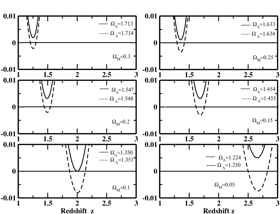
Figure 1: {$\Omega_{m}(1+z)^{3}+\Omega_{\wedge}+\Omega_{k}(1+z)^{2}\}$ versus redshift $z$ for various normalized matter densities between 0.30 and 0.05.

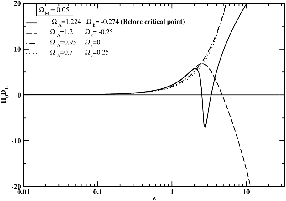
Figure 2: Plots of $H_{0}D_{L}$ as functions of log $z$ with various values of $\Omega_{\wedge}$ with $\Omega_{m}$ of 0.05 and c normalized to 1.

We have traced these inconsistencies at $\Omega_{m}$ of 0.05 and 0.30, with various values for $\Omega_{\wedge}$ and present results in Figures 2 and 3 as plots of $H_{0}D_{L}$ with respect to log$z$. Both figures demonstrate for large values of the cosmological constant, 1.2 to 1.7, and with reasonable values of spacetime curvature $\Omega_{k}$ drastic deviations from useful solutions of $H_{0}D_{L}$. At the lower matter density of 0.05 (Fig. 2) this function does not straightforwardly correlate $H_{0}D_{L}$ with $z$, for values of $\Omega_{\wedge}$ above 1.2 and for $z$ above about 2. Here the critical value for $\Omega_{\wedge}$ is a rather low 1.224. With increasing $\Omega_{\wedge}$ from 0.70 to 0.95, we find the larger values of $z$ correlate with the smaller values of $\Omega_{\wedge}$ as should be observed in a Universes with increasing matter densities and decreasing anti-matter densities. As plotted in Fig. 3 ($\Omega_{m}$= 0.30), all curves are shifted to higher values of z, as expected for a Universe more populated with matter than in Figure 2. The model appears well behaved with larger values of $H_{o}D_{L}$ correlating with larger values of redshift up to perhaps $\Omega_{\wedge}$ of 1.2; solutions of $H_{o}D_{L}$ at values of $\Omega_{\wedge}$ greater than this and above $z$ of 3.25 are questionable. Here, evaluations of $H_{0}D_{L}$ with smaller values of $\Omega_{\wedge}$ appear indiscriminate but perhaps useful up to $z$ of about 3, but no further. Beyond this redshift $z$ is predicted to correlate with anti-gravity density. Though these problems of inconsistency are for $\Omega_{\wedge}$ greater than 0.70 - just outside the range currently thought to be important - as the Universe expands, $\Omega_{\wedge}$ is supposed to dominate with $\Omega_{m}$ eventually approaching 0 and the standard model may fail for even moderate values of the redshift and $\Omega_{\wedge}$. We have found the FRW model does not obviously fail for negative values of $\Omega_{\wedge}$ over a much wider range of $\Omega_{m}$ and $z$. Figure 4 presents log $H_{0}D_{\mbox{L}}$ versus log$z$ for $\Omega_{m}$ of 0.05 with $\Omega_{\wedge}$ from +1 to -2. As expected for a Universe dominated by attractive forces, $H_{0}D_{L}$ decreases with decreasing $\Omega_{\wedge}$ and $z$ decreases with decreasing $\Omega_{\wedge}$ in smooth manners because the Hubble flow must increase with increasing drag on expansion. Note that a positive cosmological constant ($\Omega_{\wedge}$ = 1) does follow this regular pattern above redshift of 6.59 in the Universe of low matter density (0.05); greater than this distance the energy is predicted to become strongly attractive. This ordering also exists at $\Omega_{m}$ of 0.30 (Fig. 5) but is more pronounced; up to redshifts of about 3.25 a $\Omega_{\wedge}$ of +1.0 acts as anti-gravity, but at greater distance than this $\Omega_{\wedge}$ acts attractively.

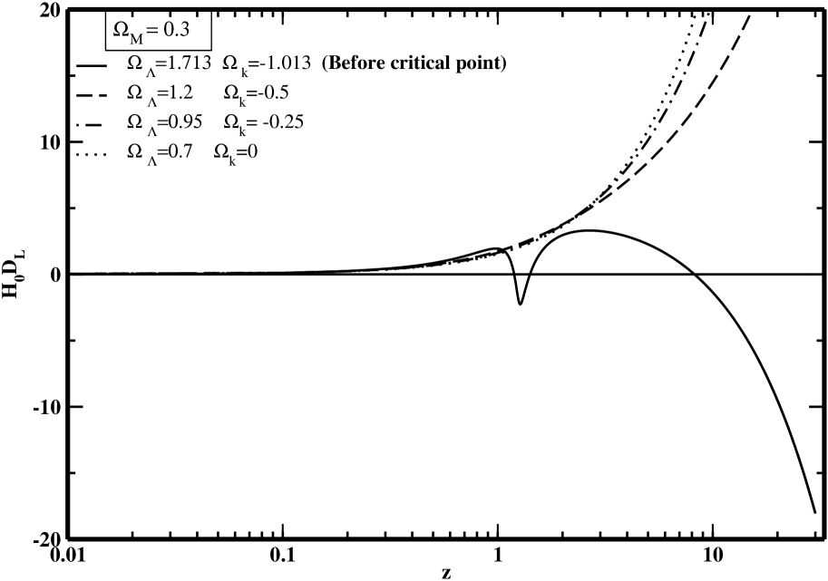
Figure 3: Plots of $H_{0}D_{L}$ as functions of log $z$ with various values of $\Omega_{\wedge}$ with $\Omega_{m}$of 0.30 and c normalized to 1.

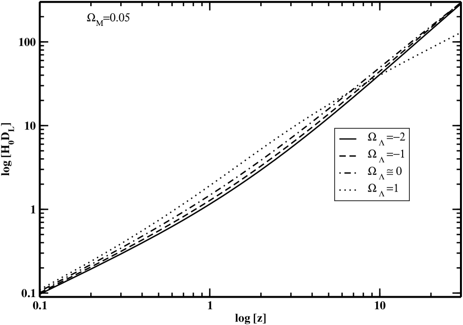
Figure 4: Log $H_{0}D_{L}$ as a function of log z for various values of $\Omega_{\wedge}$ from +1.0 to -2.0 with $\Omega_{m}$ of 0.05 and c normalized to 1. Note the ”cross-over” of the trace of the solution with $\Omega_{\wedge}$ of +1.0.

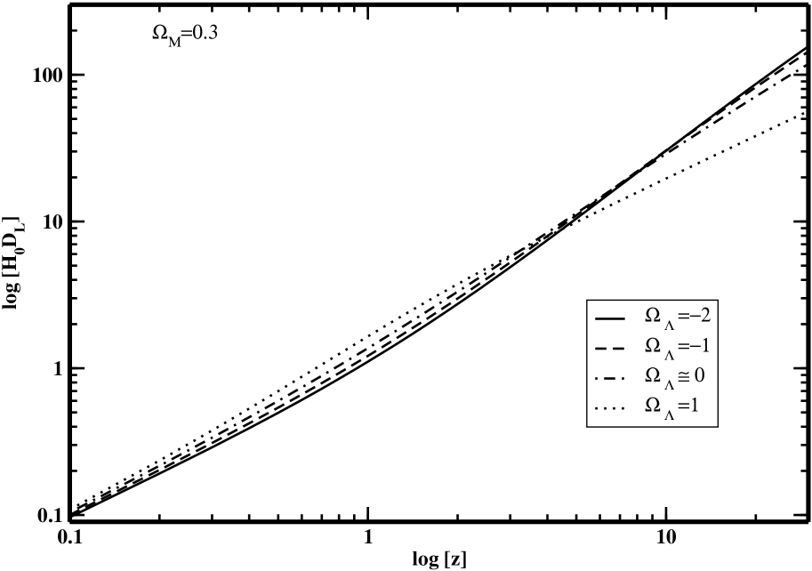
Figure 5: Log $H_{0}D_{L}$ as a function of log z for various values of $\Omega_{\wedge}$ from +1.0 to -2.0 with $\Omega_{m}$ of 0.30 and c normalized to 1. Note the ”cross-over” of the trace of the solution with $\Omega_{\wedge}$ of +1.0.

5 DISCUSSION

The selection of a solution to the standard model of cosmology using an elliptical form allows us to probe the ability of the model to estimate Hubble expansion at great distances with dependence upon $\Omega_{\wedge}$. We have found, for values of $\Omega_{\wedge}$ between 0 and -2 and values of $\Omega_{m}$ currently thought realistic, the standard model returns a consistent value for $H_{0}D_{L}$ at $z<$ 20. This is greater than redshifts currently reported for the farthest galaxies, though this value may be surpassed soon. When this model is solved for values of $\Omega_{\wedge}$ greater than 0 problems arise at high values of $z$, where positive $\Omega_{\wedge}$ acts as attractive. In regions of $\Omega_{\wedge}$ greater than +1 inconsistencies are observed of a general nature which limits the usefulness of the standard model to regions of high matter density - densities consistent with the Einstein-de Sitter model and currently thought important. If the Universe is rushing towards a state of low matter density, increasing dependence upon $\Omega_{\wedge}$ with a trace of closed curvature (preferred by Einstein among others) the standard model will probably fail. These regions of inconsistencies might be interpreted by some, as evidence for an epoch of matter dominated Universe with a low Universe expansion rate followed by the current epoch of vacuum energy domination and faster expansion, though it seems to us that earlier epochs might be best not judged using the standard model. Very unfortunately, this also means calculations of epochs of newly discovered galaxies exhibiting high redshifts will remain unreliable until the FRW model can be better adapted for greater distances. The standard model has limitations of usefulness with respect to accurate predictions of large galactic distances and Universe age. Inclusion of positive values for the vacuum energy further restricts the range of useful predictions. Other models or model variations incorporating modified application of the vacuum energy, but not suffering regions of inconsistency, might be preferred. We hope to introduce one such model soon.

ACKNOWLEDGEMENTS We are grateful for the continuing interest of Professor Jan Paul in our work.

REFERENCES Behar, S. and Carmeli, M. (2000) International Journal of Theoretical Physics 39, 1375. Bisabr, Y. (2004) International Journal of Theoretical Physics 43, 2137. Carroll, S.M., Press, W.H. and Turner, E.L. (1992) Annual Review of Astronomy and Astrophysics 30, 499. Einstein, A. (1916) Relativity, translation 2000, Routledge Classics, NY. Fall S.M. (1975) Monthly Notices of the Royal Astronomical Society 172, 23. Feldman, H. Jusziewicz, R., Ferreira, P., Davis, M., Gaztanas, E., Fry, J., Jaffee, A., Chambers, S., La Costa, L., Bernardi, M., Giovanelli, R., Haynes, M. and Wegner, G. (2003) Astrophysical Journal 596, L131. Freedman, W.L., Madore, B.F., Gibson, B.K., Ferrarese, L., Kelson, D.D., Sakai, S., Mould, J.R., Kennicutt, Jr., R.C., Ford, H.C., Graham, J.A., Huchra, J.P., Hughes, S.M.G., Illingworth, G.D., Macri, L.M. and Stetson, P.B. (2001) Astrophysical Journal 553, 47. Grundahl, F. VandenBerg, D.A., Bell, R.A., Andersen, M.I. and Stetson, P.B. (2000) Astronomical Journal 120, 1884. Kneib, J.-P., Ellis, R.S., Santos, M.R. and Ricard J. (2004) Astrophysical Journal 607, 697. Peebles, P.J.E. (1993) Principles of Physical Cosmology, Princeton University Press, Princeton, New Jersey, pp.100-102. Riess, A.G., Strolger, L-G., Tonry, J., Casertano, S., Ferguson, H.C., Mobasher, B., Challis, P., Filippenko, A.V., Jha, S., Li, W., Chornock, R., Kirshner, R.P., Leibundgut, B., Dickinson, M., Livio, M., Giavalisco, M., Steidel, C.C., Benitez, N., and Tsvetanov, Z. (2004). Astrophysical Journal 607, 665. Riess, A.D., Filippenko, A.V., Challis, P., Clocgiatti, A., Dierks, A., Garnavich, P.M., Gilliland, R.L., Hogan, C.J., Jha, S., Kirshner, R.P., Leibundgut, B., Phillips, M.M., Reiss, D., Schmidt, B.P., Schommer, R.A., Smith, R.C., Spyromilio, J., Stubbs, C., Suntzeff, N.B. and Tonry, J. (1998) Astronomical Journal 116, 1009. Tonry, J.L., Schmidt, B.P., Barris, B., Candia, P., Challis, P., Clocchiatti, A., Coil, A.L., Filippenko, A.V., Garnavich, P., Hogan, C., Holland, S.T., Jha, S., Kirshner, R.P., Krisciunas, K., Leibundgut, B., Li, W., Matheson, T., Phillips, M.M., Riess, A.G., Schommer, R., Smith, R.C., Sollerman, J., Spyromilio, J., Stubbs, C.W. and Suntzeff, N.B. (2003) Astrophysical Journal 594, 1. VandenBerg, D.O., Ricard, O., Michaud, G. and Richer J. (2002) Astrophysical Journal 571, 487.

APPENDIX

We derive equation (16), the elliptical form useful for astronomy from our equation (9). The FRW metric, allowing $a(t)=\frac{R}{R_{o}}$ is

$$\frac{dR_{o}r}{dt}=\frac{R_{o}}{R}(1-kr^{2})^{1/2}$$ (18)

$$R_{o}\frac{dr}{dt}=\frac{1}{a(t)}(1-kr^{2})^{1/2}$$ (19)

with rearrangement becomes

$$\frac{R_{o}dr}{(1-kr^{2})^{1/2}}=\frac{dt}{a(t)}.$$ (20)

Remembering that $\tau$= $H_{o}t$ we multiply through by $H_{o}$to get

$$H_{o}R_{o}\frac{dr}{(1-kr^{2})^{1/2}}=\frac{d\tau}{a(t)}$$ (21)

and multiply through again using the relationship for the normalized $\Omega_{k}=-\frac{k}{R_{0}^{2}H_{o}^{2}}$

$$H_{o}R_{o}\frac{dr}{(1+\Omega_{o}R_{o}^{2}H_{o}^{2}r^{2})^{1/2}}=\frac{d\tau}{a(t)}.$$ (22)

Substituting equation (9) for $d\tau$ we have

$$H_{o}R_{o}\frac{dr}{(1+\Omega_{o}R_{o}^{2}H_{o}^{2}r^{2})^{1/2}}=\frac{1}{a(\tau)}\frac{\sqrt{a(\tau)}da(\tau)}{\sqrt{\Omega_{m}+\Omega_{\wedge}a(\tau)^{3}+\Omega_{k}a(\tau)}}$$ (23)

and integrating both sides and rearranging some constant parameters

$$H_{o}R_{o}\int_{0}^{r_{1}}\frac{1}{\sqrt{1+\Omega_{o}R_{o}^{2}H_{o}^{2}r^{2}}}dr=\int_{a_{1}}^{1}\frac{1}{\sqrt{a(\tau)}\sqrt{\Omega_{m}+\Omega_{\wedge}a(\tau)^{3}+\Omega_{k}a(\tau)}}da(\tau)$$ (24)

then changing the variable on the left side using $y=\sqrt{\Omega_{k}}R_{o}H_{o}r$ and using the redshift relationship $a=$ $\frac{1}{(1+z)}$ for substitution of the right hand side we get

$$\frac{1}{\sqrt{\Omega_{k}}}\int_{0}^{\sqrt{\Omega_{k}}R_{0}H_{0}r_{1}}\frac{1}{\sqrt{1+y^{2}}}dy=-\int_{z_{1}}^{0}\frac{\sqrt{1+z}}{(1+z)^{2}\sqrt{\Omega_{m}+\frac{\Omega_{\wedge}}{(1+z)^{3}}+\frac{\Omega_{k}}{1+z}}}dz.$$ (25)

The integral on the left hand side is $\textrm{\rm arcsinh}(y)$ so the above becomes

$$\frac{1}{\sqrt{\Omega_{k}}}\textrm{\rm arcsinh}(\sqrt{\Omega_{k}}R_{0}H_{0}r_{1})=\int_{0}^{z_{1}}\frac{1}{\sqrt{\Omega_{m}(1+z)^{3}+\Omega_{\wedge}+\Omega_{k}(1+z)^{2}}}dz$$ (26)

and substituting to arrive at the measurable $D_{L}$ using the relationships $D_{m}=R_{o}r_{1}$ and $D_{L}=(1+z)D_{m}$ we arrive at

$$H_{o}D_{L}=\frac{1+z}{\sqrt{\left|\Omega_{k}\right|}}\sin\mbox{\bf n}\{\frac{\sqrt{\left|\Omega_{k}\right|}}{\sqrt{\Omega_{m}}}\int_{0}^{z_{1}}\frac{1}{\sqrt{(1+z)^{3}+\frac{\Omega_{\wedge}}{\Omega_{m}}+\frac{\Omega_{k}}{\Omega_{m}}(1+z)^{2}}}dz$$ (27)

and with introduction of c for the speed of light becomes our equation (16).