Error analysis in Fourier methods for option pricing

Abstract.

We provide a bound for the error committed when using a Fourier method to price European options when the underlying follows an exponential Lévy dynamic. The price of the option is described by a partial integro-differential equation (PIDE). Applying a Fourier transformation to the PIDE yields an ordinary differential equation (ODE) that can be solved analytically in terms of the characteristic exponent of the Lévy process. Then, a numerical inverse Fourier transform allows us to obtain the option price. We present a bound for the error and use this bound to set the parameters for the numerical method. We analyse the properties of the bound and demonstrate the minimisation of the bound to select parameters for a numerical Fourier transformation method to solve the option price efficiently.

1. Introduction

Lévy processes form a rich field within mathematical finance. They allow modelling of asset prices with possibly discontinuous dynamics. An early and probably the best known model involving a Lévy process is the Merton (1976) model, which generalises the Black and Scholes (1973) model. More recently, we have seen more complex models allowing for more general dynamics of the asset price. Examples of such models include the Kou (2002) model (see also Dotsis et al. (2007)), the Normal Inverse Gaussian model (Barndorff-Nielsen (1997); Rydberg (1997)), the Variance Gamma model (Madan and Seneta (1990); Madan et al. (1998)), and the Carr-Geman-Madan-Yor (CGMY) model (Carr et al. (2002, 2003)). For a good exposition on jump processes in finance we refer to Cont and Tankov (2004) (also see Raible (2000) and Eberlein (2001)).

Prices of European options whose underlying asset is driven by the Lévy process are solutions to partial integro-differential Equations (PIDEs) (Nualart et al. (2001); Briani et al. (2004); Almendral and Oosterlee (2005); Kiessling and Tempone (2011)) that generalise the Black-Scholes equation by incorporating a non-local integral term to account for the discontinuities in the asset price. This approach has also been extended to cases where the option price features path dependence, for instance in Boyarchenko and Levendorskiǐ (2002) d’Halluin et al. (2004) and Lord et al. (2008).

The Lévy -Khintchine formula provides an explicit representation of the characteristic function of a Lévy process (cf, Tankov (2004)). As a consequence, one can derive an exact expression for the Fourier transform of the solution of the relevant PIDE. Using the inverse fast Fourier transform (iFFT) method, one may efficiently compute the option price for a range of asset prices simultaneously. Furthermore, in the case of European call options, one may use the duality property presented by Dupire (1997) and iFFT to efficiently compute option prices for a wide range of strike prices.

Despite the popularity of Fourier methods for option pricing, few works can be found on the error analysis and related parameter selection for these methods. A bound for the error not only provides an interval for the precise value of the option, but also suggests a method to select the parameters of the numerical method. An important work in this direction is the one by Lee (2004) in which several payoff functions are considered for a rather general set of models, whose characteristic function is assumed to be known. Feng and Linetsky (2008) presents the framework and theoretical approach for the error analysis, and establishes polynomial convergence rates for approximations of the option prices. For a more contemporary review on the error committed in various FT-related methods we refer the reader to Boyarchenko and Levendorskii (2011), that extends the classical flat Fourier methods by deforming the integration countours on the complex plane, studying discretely monitored barrier options studied in De Innocentis and Levendorskii (2014).

In this work, we present a methodology for studying and bounding the error committed when using FT methods to compute option prices. We also provide a systematic way of choosing the parameters of the numerical method, in a way that minimises the strict error bound, thus guaranteeing adherence to a pre-described error tolerance. We focus on exponential Lévy processes that may be of either diffusive or pure jump. Our contribution is to derive a strict error bound for a Fourier transform method when pricing options under risk-neutral Lévy dynamics. We derive a simplified bound that separates the contributions of the payoff and of the process in an easily processed and extensible product form that is independent of the asymptotic behaviour of the option price at extreme prices and at strike parameters. We also provide a proof for the existence of optimal parameters of the numerical computation that minimise the presented error bound. When comparing our work with Lee’s work we find that Lee’s work is more general than ours in that he studies a wider range of processes, on the other hand, our results apply to a larger class of payoffs. On test examples of practical relevance, we also find that the bound presented produces comparable or better results than the ones previously presented in the literature, with acceptable computational cost.

The paper is organised in the following sections: In Section 2 we introduce the PIDE setting in the context of risk-neutral asset pricing; we show the Fourier representation of the relevant PIDE for asset pricing with Lévy processes and use that representation for derivative pricing. In Section 3 we derive a representation for the numerical error and divide it into quadrature and cutoff contributions. We also describe the methodology for choosing numerical parameters to obtain minimal error bounds for the FT method. The derivation is supported by numerical examples using relevant test cases with both diffusive and pure-jump Lévy processes in Section 4. Numerics are followed by conclusions in Section 5.

2. Fourier method for option pricing

Consider an asset whose price at time $t$ is modelled by the stochastic process $S=(S_{t})$ defined by $S_{t}=S_{0}e^{X_{t}}$, where $X=(X_{t})\in\mathbb{R}$ is assumed to be a Lévy process whose jump measure $\nu$ satisfies

(1) $$\int_{\mathbb{R}\setminus\left\{{0}\right\}}\min\{y^{2},1\}\nu\left({dy}\right)<\infty$$

Assuming the risk-neutral dynamic for $S_{t}$, the price at time $t=T-\tau$ of a European option with payoff $G$ and maturity time $T$ is given by

$$\Pi(\tau,s)=e^{-r\tau}\mathrm{E}\left({{G\left({S_{T}}\right)|S_{T-\tau}=s}}\right)$$

where $r$ is the short rate that we assume to be constant and $\tau\colon 0\leq\tau\leq T$ is the time to maturity. Extensions to non-constant deterministic short rates are straightforward.

The infinitesimal generator of a Lévy process $X$ is given by (see Applebaum, 2004)

$$\mathcal{L}^{X}f(x) \equiv\lim_{h\to 0}\frac{\mathrm{E}\left({{f(X_{t+h})|X_{t}=x}}\right)-f(x)}{h}$$

(2) $$=\gamma f^{\prime}(x)+\frac{1}{2}\sigma^{2}f^{\prime\prime}(x)+\int_{\mathbb{R}\setminus\left\{{0}\right\}}\left(f(x+y)-f(x)-y1_{|y|\leq 1}f^{\prime}(x)\right)\nu(\textrm{d}y)$$

where $(\gamma,\sigma^{2},\nu)$ is the characteristic triple of the Lévy process. The risk-neutral assumption on $(S_{t})$ implies

(3) $$\int_{\left|{y}\right|>1}e^{y}\nu(\textrm{d}y)<\infty$$

and fixes the drift term (see Kiessling and Tempone (2011)) $\gamma$ of the Lévy process to

(4) $$\gamma=r-\frac{1}{2}\sigma^{2}-\int_{\mathbb{R}\setminus\left\{{0}\right\}}\left({e^{y}-1-y1_{|y|\leq 1}}\right)\nu(\textrm{d}y)$$

Thus, the infinitesimal generator of $X$ may be written under the risk-neutral assumption as

(5) $$\mathcal{L}^{X}f(x) =\left(r-\frac{\sigma^{2}}{2}\right)f^{\prime}(x)+\frac{\sigma^{2}}{2}f^{\prime\prime}(x)+\int_{\mathbb{R}\setminus\left\{{0}\right\}}\left(f(x+y)-f(x)-(e^{y}-1)f^{\prime}(x)\right)\nu(\textrm{d}y)$$

Consider $g$ as the reward function in log prices (ie, defined by $g(x)=G(S_{0}e^{x})$). Now, take $f$ to be defined as

$$f\left({\tau,x}\right)\equiv\mathrm{E}\left({{g\left({X_{T}}\right)|X_{T-\tau}=x}}\right)$$

Then $f$ solves the following PIDE:

$$\begin{cases}\partial_{\tau}f(\tau,x)&=\mathcal{L}^{X}f(\tau,x)\\ f(0,x)&=g(x),\qquad\qquad\left({\tau,x}\right)\in[0,T]\times\mathbb{R}\end{cases}$$

Observe that $f$ and $\Pi$ are related by

(6) $$\Pi(\tau,S_{0}e^{x})=e^{-r\tau}f(\tau,x)$$

Consider a damped version of $f$ defined by $f_{\alpha}(\tau,x)=e^{-\alpha x}f(\tau,x)$; we see that $\partial_{\tau}f_{\alpha}=e^{-\alpha x}\mathcal{L}^{X}f\left({\tau,x}\right)$.

There are different conventions for the Fourier transform. Here we consider the operator $\operatorname{\mathcal{F}}$ such that

(7) $$\operatorname{\mathcal{F}}[f]\left({\omega}\right)\equiv\int_{\mathbb{R}}e^{i\omega x}f\left({x}\right)\textrm{d}x$$

defined for functions $f$ for which the previous integral is convergent. We also use $\hat{f}\left({\omega}\right)$ as a shorthand notation of $\operatorname{\mathcal{F}}[f]\left({\omega}\right)$. To recover the original function $f$, we define the inverse Fourier transform as

$$\operatorname{\mathcal{F}^{-1}}\left[f\right](x)=\frac{1}{2\pi}\int_{\mathbb{R}}e^{-i\omega x}f(\omega)\textrm{d}\omega$$

We have that $\operatorname{\mathcal{F}^{-1}}\left[\hat{f}\right](x)=f(x)$.

Applying $\operatorname{\mathcal{F}}$ to $f_{\alpha}$ we get $\hat{f_{\alpha}}(\omega)=\hat{f}\left({\omega+i\alpha}\right)$. Observe also that the Fourier transform applied to $\mathcal{L}^{X}f(\tau,x)$ gives $\Psi\left({{-i\omega}}\right)\hat{f}\left({\tau,\omega}\right)$, where $\Psi\left({{\cdot}}\right)$ is the characteristic exponent of the process $X$, which satisfies $\mathrm{E}\left({{e^{zX_{t}}}}\right)=e^{t\Psi\left({{z}}\right)}$. The explicit expression for $\Psi\left({{\cdot}}\right)$ is

(8) $$\Psi\left({{z}}\right)=\left({r-\frac{\sigma^{2}}{2}}\right)z+\frac{\sigma^{2}}{2}z^{2}+\int_{\mathbb{R}}\left(e^{zy}-1-(e^{y}-1)z\right)\nu(\textrm{d}y)\\$$

From the previous considerations it can be concluded that

(9) $$\partial_{\tau}\hat{f_{\alpha}}=\Psi\left({{\alpha-i\omega}}\right)\hat{f}\left({\omega-i\alpha}\right)$$

Now $\hat{f}\left({\omega-i\alpha}\right)=\hat{f_{\alpha}}\left({\omega}\right)$ so $\hat{f_{\alpha}}$ satisfies the following ODE

(10) $$\begin{cases}\frac{\partial_{\tau}\hat{f_{\alpha}}\left({\tau,\omega}\right)}{\hat{f_{\alpha}}(\tau,\omega)}&=\Psi\left({{\alpha-i\omega}}\right)\\[5.0pt] \hat{f_{\alpha}}\left({0,\omega}\right)&=\hat{g_{\alpha}}\left({\omega}\right)\end{cases}$$

Solving the previous ODE explicitly, we obtain

(11) $$\hat{f_{\alpha}}\left({\tau,\omega}\right)=e^{\tau\Psi\left({{\alpha-i\omega}}\right)}\hat{g_{\alpha}}\left({\omega}\right)$$

Observe that the first factor in the right-hand side in the above equation is $\mathrm{E}\left({{e^{\left({\alpha-i\omega}\right)X_{\tau}}}}\right)$, (ie, $\varphi_{1}\left({{-i\alpha-\omega}}\right)$), where $\varphi_{\tau}\left({{\cdot}}\right)$ denotes the characteristic function of the random variable $X_{\tau}$

(12) $$\varphi_{\tau}\left({{\omega}}\right)\equiv\mathrm{E}\left({{\tau\Psi\left({{i\omega}}\right)}}\right)$$

Now, to obtain the value function we employ the inverse Fourier transformation, to obtain

(13) $$f_{\alpha}(\tau,x)=\operatorname{\mathcal{F}^{-1}}\left[\hat{f_{\alpha}}\right](\tau,x)=\frac{1}{2\pi}\int_{\mathbb{R}}e^{-i\omega x}\hat{f_{\alpha}}(\tau,\omega)d\omega$$

or

(14) $$f_{\alpha}(\tau,x)=\frac{1}{\pi}\int_{0}^{+\infty}e^{-i\omega x}\hat{f_{\alpha}}(\tau,\omega)d\omega$$

As it is typically not possible to compute the inverse Fourier transform analytically, we approximate it by discretising and truncating the integration domain using trapezoidal quadrature (13). Consider the following approximation:

(15) $$f_{\alpha,\Delta\omega,n}(\tau,x) =\frac{\Delta\omega}{2\pi}\sum_{k=-n}^{n-1}e^{-i{\left({k+\frac{1}{2}}\right)\Delta\omega}x}\hat{f_{\alpha}}\left({\tau,{\left({k+\frac{1}{2}}\right)\Delta\omega}}\right)$$

(16) $$=\frac{\Delta\omega}{\pi}\sum_{k=0}^{n-1}e^{-i{\left({k+\frac{1}{2}}\right)\Delta\omega}x}\hat{f_{\alpha}}\left({\tau,{\left({k+\frac{1}{2}}\right)\Delta\omega}}\right)$$

Bounding and consequently minimising the error in the approximation of $f(\tau,x)$ by

$$f_{\Delta\omega,n}(\tau,x)\equiv e^{\alpha x}f_{\alpha,\Delta\omega,n}(\tau,x)$$

is the main focus of this paper and will be addressed in the following section.

Remark 2.1.

Although we are mainly concerned with option pricing when the payoff function can be damped in order to guarantee regularity in the $L^{1}$ sense, we note here that our main results are naturally extendable to include the Greeks of the option. Indeed, we have by (11) that

(17) $$f\left({t,x}\right)=\frac{1}{2\pi}\int_{\mathbb{R}}e^{\left({\alpha-i\omega}\right)x}\hat{f_{\alpha}}\left({\tau,\omega}\right)\textrm{d}\omega$$

so the Delta and Gamma of the option equal

(18) $$\Delta\left({t,x}\right) \equiv\frac{\partial f\left({t,x}\right)}{\partial x}=\frac{1}{2\pi}\int_{\mathbb{R}}\left({\alpha-i\omega}\right)e^{\left({\alpha-i\omega}\right)x}\hat{f_{\alpha}}\left({\tau,\omega}\right)\textrm{d}\omega$$

(19) $$\Gamma\left({t,x}\right) \equiv\frac{\partial^{2}f\left({t,x}\right)}{\partial x^{2}}=\frac{1}{2\pi}\int_{\mathbb{R}}\left({\alpha-i\omega}\right)^{2}e^{\left({\alpha-i\omega}\right)x}\hat{f_{\alpha}}\left({\tau,\omega}\right)\textrm{d}\omega$$

Because the expressions involve partial derivatives with respect to only $x$, the results in this work are applicable for the computation of $\Delta$ and $\Gamma$ through a modification of the payoff function:

(20) $$\hat{g}_{\alpha,\Delta}\left({\omega}\right)= \hat{g}_{\alpha}\left({\omega}\right)\left({\alpha-i\omega}\right)$$

(21) $$\hat{g}_{\alpha,\Gamma}\left({\omega}\right)= \hat{g}_{\alpha}\left({\omega}\right)\left({\alpha-i\omega}\right)^{2}$$

When the Fourier space payoff function manifests exponential decay, the introduction of a coefficient that is polynomial in $\omega$ does not change the regularity of $\hat{g}$ in a way that would significantly change the following analysis. Last, we note that since we do our analysis for PIDEs on a mesh of $x$’s, one may also compute the option values in one go and obtain the Greeks with little additional effort using a finite difference approach for the derivatives.

2.1. Evaluation of the method for multiple values of $x$ simultaneously

The Fast Fourier Transform (FFT) algorithm provides an efficient way of computing (15) for an equidistantly spaced mesh of values for $x$ simultaneously. Examples of works that consider this widely extended tool are Lord et al. (2008); Jackson et al. (2008); Hurd and Zhou (2010) and Schmelzle (2010).

Similarly, one may define the Fourier frequency $\omega$ as the conjugate variable of some external parameter on which the payoff depends. Especially, for the practically relevant case of call options, we can denote the log-strike as $k$ and treat $x$ as a constant and write:

(22) $$\tilde{f}_{k,\alpha}\left({\omega}\right)\equiv\int_{\mathbb{R}}e^{\left({\alpha+i\omega}\right)k}f_{k}\left({x}\right)\textrm{d}k$$

Using this convention, the time dependence is given by

(23) $$\tilde{f}_{k,\alpha}\left({\tau,x}\right)=\frac{e^{\left({i\omega+\alpha+1}\right)x}\varphi_{\tau}\left({{\omega-i\left({\alpha+1}\right)}}\right)}{\left({i\omega+\alpha}\right)\left({i\omega+\alpha+1}\right)}$$

contrasted with the $x$-space solution

(24) $$\hat{f}_{k,\alpha}\left({\tau,x}\right)=\frac{e^{\left({i\omega-\alpha+1}\right)k}\varphi_{\tau}\left({{\omega+i\alpha}}\right)}{\left({i\omega+\alpha}\right)\left({i\omega+\alpha+1}\right)}$$

We note that for call option payoff to be in $L^{1}$, we demand that $\alpha$ in (23) is positive. Omitting the exponential factors that contain the $x$ and $k$ dependence in (23) and (24) respectively, we have that one can arrive from (23) to (24) using the mapping $\alpha\mapsto-\alpha-1$. Thanks to this, much of the analysis regarding the $x$-space transformation generalises in a straightforward manner to the $k$-space transform.

3. Error bound

The aim of this section is to compute a bound of the error when approximating the option price $f(\tau,x)$ by $f_{\alpha,\Delta\omega,n}(\tau,x)$, defined in (15). Considering

(25) $$f_{\alpha,\Delta\omega}(\tau,x)=\frac{\Delta\omega}{2\pi}\sum_{k\in\mathbf{Z}}e^{-i{\left({k+\frac{1}{2}}\right)\Delta\omega}x}\hat{f_{\alpha}}\left({\tau,{\left({k+\frac{1}{2}}\right)\Delta\omega}}\right)$$

the total error $\mathcal{E}$ can be split into a sum of two terms: the quadrature and truncation errors. The former is the error from the approximation of the integral in (13) by the infinite sum in (25), while the latter is due to the truncation of the infinite sum. Using triangle inequality, we have

(26) $$\mathcal{E} :=\left|{f(\tau,x)-f_{\Delta\omega,n}(\tau,x)}\right|\leq\mathcal{E_{Q}}+\mathcal{E_{F}}$$

with

$$\mathcal{E_{Q}} =e^{\alpha x}\left|{f_{\alpha}(\tau,x)-f_{\alpha,\Delta\omega}(\tau,x)}\right|$$

$$\mathcal{E_{F}} =e^{\alpha x}\left|{f_{\alpha,\Delta\omega}(\tau,x)-f_{\alpha,\Delta\omega,n}(\tau,x)}\right|$$

Observe that each $\mathcal{E}$, $\mathcal{E_{Q}}$ and $\mathcal{E_{F}}$ depend on three kinds of parameters:

• Parameters underlying the model and payoff such as volatility and strike price. We call these physical parameters.

• Parameters relating to the numerical scheme such as $\alpha$ and $n$.

• Auxiliary parameters that will be introduced in the process of deriving the error bound. These parameters do not enter the computation of the option price, but they need to be chosen appropriately to have as tight a bound as possible.

We start by analysing the quadrature error.

3.1. Quadrature error

Denote by $A_{a}$, with $a>0$, the strip of width $2a$ around the real line:

$$A_{a}\equiv\left\{z\in\mathbb{C}\colon\left|{\mathrm{Im}\left[z\right]}\right|<a\right\}$$

The following theorem presents conditions under which the quadrature error goes to zero at a spectral rate as $\Delta\omega$ goes to zero. Later in this section, we discuss simpler conditions to verify the hypotheses and analyse in more detail the case when the process $X$ is a diffusive process or there are “enough small jumps.”

Theorem 3.1.

Assume that for $a>0$:

• the characteristic function of the random variable $X_{1}$ has an analytic extension to the set

  $$A_{a}-\alpha i\equiv\left\{z\in\mathbb{C}\colon\left|{\mathrm{Im}\left[z\right]+\alpha}\right|<a\right\}$$

• the Fourier transform of $g_{\alpha}(x)$ is analytic in the strip $A_{a}$ and

• there exists a continuous function $\gamma\in L^{1}(\mathbb{R})$ such that $\left|{\hat{f_{\alpha}}(\tau,\omega+i\beta)}\right|<\gamma(\omega)$ for all $\omega\in\mathbb{R}$ and for all $\beta\in[-a,a]$

Then the quadrature error is bounded by

$$\mathcal{E_{Q}}\leq e^{\alpha x}\frac{M_{\alpha,a}(\tau,x)}{2\pi\left({e^{2\pi a/\Delta\omega}-1}\right)}$$

where $M_{\alpha,a}(\tau,x)$ is given by

(27) $$M_{\alpha,a}(\tau,x) :=\sum_{\beta\in\{-a,a\}}\int_{\mathbb{R}}\left|{e^{-i\left({\omega+i\beta}\right)x}\hat{f_{\alpha}}(\tau,\omega+i\beta)}\right|\textrm{d}\omega$$

$M_{\alpha,a}(\tau,x)$ equals the Hardy norm (defined in (28)) of the function $\omega\mapsto e^{-i\left({\omega+i\beta}\right)x}\hat{f_{\alpha}}(\tau,\omega+i\beta)$, which is finite.

The proof of Theorem 3.1 is an application of Theorem 3.2.1 in Stenger (1993), whose relevant parts we include for ease of reading. Using the notation in Stenger (1993), $H^{1}_{A_{a}}$ is the family of functions $w$ that are analytic in $A_{a}$ and such that

(28) $$\left|{\left|{{w}}\right|}\right|_{H^{1}_{A_{a}}}:=\lim_{\varepsilon\to 0}\int_{\partial A_{a}(\varepsilon)}\left|{w(z)}\right|d\left|{z}\right|<\infty$$

where

$$A_{a}(\varepsilon)=\left\{z\in\mathbb{C}\colon\left|{z}\right|<\frac{1}{\varepsilon},\ \left|{\mathrm{Im}\left[z\right]}\right|<a\left({1-\varepsilon}\right)\right\}$$

Lemma 3.2 (Theorem 3.2.1 in Stenger (1993)).

Let $w\in H^{1}_{A_{a}}$, then define:

(29) $$I\left({w}\right) =\int_{\mathbb{R}}w\left({x}\right)\textrm{d}x$$

(30) $$J\left({w,h}\right) =h\displaystyle\sum\limits_{j=-N}^{N}w\left({jh}\right)$$

(31) $$\zeta\left({w,h}\right) =I\left({w}\right)-J\left({w,h}\right)$$

then

(32) $$\left|{\zeta\left({w,h}\right)}\right|\leq\frac{e^{-\frac{\pi a}{h}}\left|{\left|{{w}}\right|}\right|_{H^{1}_{A_{a}}}}{2\mathrm{sinh}\left({\frac{\pi a}{h}}\right)}$$

Proof of Theorem 3.1.

First observe that H1 and H2 imply that the function $w(z)=e^{-ixz+\Delta\omega/2}\hat{f_{\alpha}}(\tau,z+\Delta\omega/2)$ is analytic in $A_{a}$. H3 allows us to use dominated convergence theorem to prove that $\left|{\left|{{w}}\right|}\right|_{H^{1}_{A_{a}}}$ is finite and coincides with $M_{\alpha,a}(\tau,x)$. Applying Lemma 3.2 the proof is completed. ∎

Regarding the hypotheses of Theorem 3.1, the next propositions provide simpler conditions that imply H1 and H2 respectively.

Proposition 3.3.

If $\alpha$, $a$ and $\nu$ are such that

(33) $$\int_{y>1}e^{\left({\alpha+a}\right)y}\nu(\textrm{d}y)<\infty\quad\text{and}\quad\int_{y<-1}e^{\left({\alpha-a}\right)y}\nu(\textrm{d}y)<\infty$$

then H1 in Theorem 3.1 is fulfilled.

Proof.

Denoting by $\varphi_{1}\left({{\cdot}}\right)$ the characteristic function of $X_{1}$, we want to prove that $z\mapsto\varphi_{1}\left({{z+\alpha i}}\right)$ is analytic in $A_{a}$. Considering that $\varphi_{1}\left({{z+\alpha i}}\right)=e^{\Psi\left({{iz-\alpha}}\right)}$, the only non-trivial part of the proof is to verify that

(34) $$z\mapsto\int p(z,y)\nu(\textrm{d}y)$$

is analytic in $A_{a}$, where $p\colon A_{a}\times\mathbb{R}\to\mathbb{C}$ is given by

$$p(z,y)=e^{y\left({iz-\alpha}\right)}-1-(e^{y}-1)\left({iz-\alpha}\right)$$

To prove this fact, we show that we can apply the main result and the only theorem in Mattner (2001), which, given a measure space $(\Omega,\mathcal{A},\mu)$ and an open subset $G\subseteq\mathbb{C}$, ensures the analyticity of $\int f(\cdot,\omega)d\mu(\omega)$, provided that $f\colon G\times\Omega\to\mathbb{C}$ satisfies: $f(z,\cdot)$ is $\mathcal{A}$-measurable for all $z\in G$; $f(\cdot,\omega)$ is holomorfic for all $\omega\in\Omega$; and $\int\left|{f(\cdot,\omega)}\right|d\mu(\omega)$ is locally bounded. In our case we consider the measure space to be $\mathbb{R}$ with the Borel $\sigma$-algebra and the Lebesgue measure, $G=A_{a}$ and $f=p$. It is clear that $p(x,\cdot)$ is Borel measurable and $p(\cdot,y)$ is holomorphic. It remains to verify that

$$z\mapsto\int_{\mathbb{R}^{*}}\left|{p(z,y)}\right|\nu(\textrm{d}y)$$

is locally bounded. To this end, we assume that $z<b$ (and, since $z\in A_{a}$, $\mathrm{Im}\left[z\right]<a$) and split the integration domain in $\left|{y}\right|>1$ and ${0<\left|{y}\right|\leq 1}$ to prove that both integrals are uniformly bounded.

Regarding the integral in ${\left|{y}\right|>1}$, we observe that

(35) $$\left|{p(z,y)}\right|\leq e^{y(\alpha+\mathrm{Im}\left[z\right])}+1+(e^{y}+1)(\alpha+a+b)$$

for $y<-1$ we have $e^{y(\alpha+\mathrm{Im}\left[z\right])}<e^{y(\alpha-a)}$ while for $y>1$ we have $e^{y(\alpha+\mathrm{Im}\left[z\right])}<e^{y(\alpha+a)}$. Using the previous bounds and the hypotheses together with (1) and (3), we obtain the needed bound.

For the integral in ${0<\left|{y}\right|\leq 1}$, observe that, denoting $f(z,y)=\left|{p(z,y)}\right|$, we have, $f(z,0)=0$ for every $z$, $\partial_{y}f(z,0)=0$ for every $z$, and $\left|{\partial_{yy}f(z,y)}\right|<c$ for $z\in A_{a},z<b,\left|{y}\right|<1$. From these observations we get that the McLaurin polynomial of degree one of $y\mapsto f(z,y)$ is null for every $z$, and we can bound $f(z,y)$ by the remainder term, which, in our region of interest, is bounded by $\frac{c}{2}y^{2}$, obtaining

(36) $$\int_{0<\left|{y}\right|\leq 1}\left|{p(z,y)}\right|\nu(\textrm{d}y)\leq\frac{c}{2}\int_{0<\left|{y}\right|\leq 1}y^{2}\nu(\textrm{d}y)$$

which is finite by hypothesis on $\nu$, which finishes the proof. ∎

Proposition 3.4.

If for all $b<a$, the function $x\mapsto e^{b\left|{x}\right|}{g_{\alpha}(x)}$ is in $L^{2}(\mathbb{R})$ then H2 in Theorem 3.1 is fulfilled.

Proof.

The proof is a direct application of Theorem IX.13 in Reed and Simon (1975) ∎

We now turn our attention to a more restricted class of Levy processes. Namely, processes such that either $\sigma^{2}>0$ or there exists $\lambda\in(0,2)$ such that $C\left({\lambda}\right)$ defined in (37) is strictly positive. For this class of processes, we can state our main result explicitly in terms of the characteristic triplet.

Given $\lambda\in(0,2)$, define $C\left({\lambda}\right)$ as

(37) $$C\left({\lambda}\right)=\textrm{inf}_{\kappa>1}\left\{\kappa^{\lambda}\int_{0<|y|<\frac{1}{\kappa}}y^{2}\nu(\textrm{d}y)\right\}$$

Observe that $C\left({\lambda}\right)\geq 0$ and, by our assumptions on the jump measure $\nu$, $C\left({\lambda}\right)$ is finite. Furthermore, if $\lambda\in(0,2)$ is such that

(38) $$\liminf_{\epsilon\downarrow 0}\frac{1}{\epsilon^{\lambda}}\int_{0<|y|<\epsilon}y^{2}\nu(\textrm{d}y)>0$$

then $C\left({\lambda}\right)>0.$ To see this, observe that (38) implies the existence of $\epsilon_{0}$ such that

$$\inf_{\epsilon\leq\epsilon_{0}}\left\{\frac{1}{\epsilon^{\lambda}}\int_{0<|y|<\epsilon}y^{2}\nu(\textrm{d}y)\right\}>0$$

If $\epsilon_{0}<1$ observe that

$$\inf_{\epsilon_{0}\leq\epsilon\leq 1}\left\{\frac{1}{\epsilon^{\lambda}}\int_{0<|y|<\epsilon}y^{2}\nu(\textrm{d}y)\right\}\geq\int_{0<|y|<\epsilon_{0}}y^{2}\nu(\textrm{d}y)>0$$

where for the first inequality it was taken into account that $\frac{1}{\epsilon^{\lambda}}\geq 1$ and that the integral is increasing with $\epsilon$. Combining the two previous infima and considering $\left|{\kappa}\right|=\frac{1}{\epsilon}$ we get that $C\left({\lambda}\right)>0.$

Furthermore, we note that for a Lévy model with finite jump intensity, such as the Black-Scholes and Merton models that satisfy the first of our assumption, $C\left({\lambda}\right)=0$ for all $\lambda\in(0,2)$.

Theorem 3.5.

Assume that: $\alpha$ and $a$ are such that (33) holds; $\hat{g_{\alpha}}\in L^{\infty}_{A_{a}}$; and either $\sigma^{2}>0$ or $C\left({\lambda}\right)>0$ for some $\lambda\in(0,2)$. Then the quadrature error is bounded by

$$\mathcal{E_{Q}}\leq e^{\alpha x}\frac{\tilde{M}_{\alpha,a}(\tau,x)}{2\pi\left({e^{2\pi a/\Delta\omega}-1}\right)}$$

where

(39) $$\tilde{M}_{\alpha,a}\left({\tau,x}\right)=\displaystyle\sum\limits_{c\in\left\{{-1,1}\right\}}e^{cax}e^{\tau\Psi\left({ca}\right)}\left|{\hat{g_{\alpha}}\left({ca}\right)}\right|\int_{\mathbb{R}}e^{-\tau\left(\frac{\sigma^{2}}{2}\omega^{2}+\frac{|\omega|^{2-\lambda}}{4}C\left({\lambda}\right)\mathbf{1}_{\left|{\omega}\right|>1}\right)}\textrm{d}\omega$$

Furthermore, if $\sigma^{2}>0$ we have

(40) $$\tilde{M}_{\alpha,a}\left({\tau,x}\right)\leq\frac{\sqrt{2\pi}}{\sigma\sqrt{\tau}}\displaystyle\sum\limits_{c\in\left\{{-1,1}\right\}}e^{cax}e^{\tau\Psi\left({ca}\right)}\left|{\hat{g_{\alpha}}\left({ca}\right)}\right|$$

Proof.

Considering $h_{\alpha,a}(\tau,x,\omega)$ defined by

(41) $$h_{\alpha,a}\left({\tau,x,\omega}\right)=\displaystyle\sum\limits_{c\in\left\{{-1,1}\right\}}\left|{e^{-i\left({\omega+ica}\right)x}\hat{f_{\alpha}}(\tau,\omega+ica)}\right|$$

we have that

$$M_{\alpha,a}(\tau,x)=\int_{\mathbb{R}}h_{\alpha,a}\left({\tau,x,\omega}\right)d\omega$$

On the other hand, for $\beta\in(-a,a)$:

(42) $$\left|{e^{-i\left({\omega+i\beta}\right)x}\hat{f_{\alpha}}(\tau,\omega+i\beta)}\right|=e^{\beta x}\left|{\hat{f_{\alpha}}(\tau,\omega+i\beta)}\right|=e^{\beta x}\left|{e^{\tau\Psi\left({{\alpha+\beta-i\omega}}\right)}}\right|\left|{\hat{g_{\alpha}}\left({\omega+i\beta}\right)}\right|$$

For the factor involving the characteristic exponent we have

(43) $$\left|{e^{\tau\Psi\left({{\alpha+\beta-i\omega}}\right)}}\right|=e^{\tau\Psi\left({{\alpha+\beta-i\omega}}\right)}$$

Now, observe that

$$\Psi\left({{\alpha+\beta-i\omega}}\right) =\left({\alpha+\beta}\right)\left({r-\frac{\sigma^{2}}{2}}\right)+\frac{\sigma^{2}}{2}\left({\left({\alpha+\beta}\right)^{2}-\omega^{2}}\right)$$

(44) $$\quad+\int_{\mathbb{R}\setminus\left\{{0}\right\}}\left({e^{\left({\alpha+\beta}\right)y}\cos(-y\omega)-1-\left({\alpha+\beta}\right)\left({e^{y}-1}\right)}\right)\nu(\textrm{d}y)$$

If $|\omega|\leq 1$ we bound $\cos(-y\omega)$ by 1, getting

$$\Psi\left({{\alpha+\beta-i\omega}}\right) \leq\left({\alpha+\beta}\right)\left({r-\frac{\sigma^{2}}{2}}\right)+\frac{\sigma^{2}}{2}\left({\left({\alpha+\beta}\right)^{2}-\omega^{2}}\right)$$

$$\quad+\int_{\mathbb{R}\setminus\left\{{0}\right\}}\left({e^{\left({\alpha+\beta}\right)y}-1-\left({\alpha+\beta}\right)\left({e^{y}-1}\right)}\right)\nu(\textrm{d}y)$$

(45) $$=\Psi\left({{\alpha+\beta}}\right)-\frac{\sigma^{2}}{2}\omega^{2}$$

Assume $|\omega|>1$. Using that for $|x|<1$ it holds that $\textrm{cos}(x)<1-x^{2}/4$, we can bound the first term of the integral in the following manner:

$$\int_{\mathbb{R}\setminus\left\{{0}\right\}}e^{\left({\alpha+\beta}\right)y}\cos(y\omega)\nu(\textrm{d}y) \leq\int_{0<|y|<1/|\omega|}e^{\left({\alpha+\beta}\right)y}\left(1-\omega^{2}y^{2}/4\right)\nu(\textrm{d}y)$$

$$\quad+\int_{|y|\geq 1/|\omega|}e^{\left({\alpha+\beta}\right)y}\nu(\textrm{d}y)$$

$$\leq\int_{\mathbb{R}\setminus\left\{{0}\right\}}e^{\left({\alpha+\beta}\right)y}\nu(\textrm{d}y)-\frac{|\omega|^{2-\lambda}}{4}|\omega|^{\lambda}\int_{0<|y|<1/|\omega|}y^{2}\nu(\textrm{d}y)$$

(46) $$\quad\leq\int_{\mathbb{R}\setminus\left\{{0}\right\}}e^{\left({\alpha+\beta}\right)y}\nu(\textrm{d}y)-\frac{|\omega|^{2-\lambda}}{4}C\left({\lambda}\right)$$

Inserting (46) back into (44) we get

$$\Psi\left({{\alpha+\beta-i\omega}}\right) \leq\left({\alpha+\beta}\right)\left({r-\frac{\sigma^{2}}{2}}\right)+\frac{\sigma^{2}}{2}\left({\left({\alpha+\beta}\right)^{2}-\omega^{2}}\right)$$

$$\quad+\int_{\mathbb{R}\setminus\left\{{0}\right\}}\left({e^{\left({\alpha+\beta}\right)y}-1-\left({\alpha+\beta}\right)\left({e^{y}-1}\right)}\right)\nu(\textrm{d}y)$$

$$\quad\quad-\frac{|\omega|^{2-\lambda}}{4}C\left({\lambda}\right)$$

$$=\Psi\left({{\alpha+\beta}}\right)-\frac{\sigma^{2}}{2}\omega^{2}-\frac{|\omega|^{2-\lambda}}{4}C\left({\lambda}\right)$$

Taking the previous considerations and integrating in $\mathbb{R}$ with respect to $\omega$, we obtain (39).

Finally, observing that $C\left({\lambda}\right)\geq 0$ and bounding it by 0, the bound (40) is obtained by evaluating the integral. ∎

Remark 3.6.

In the case of call options, hypothesis H2 implies a dependence between the strip-width parameter $a$ and damping parameter $\alpha$. We have that the damped payoff of the call option is in $L^{1}\left({\mathbb{R}}\right)$ if and only if $\alpha>1$ and hence the appropriate choice of strip-width parameter is given by $0<a<\alpha-1$. A similar argument holds for the case of put options, for which the Fourier-transformed damped payoff is identical to the calls with the distinction that $\alpha<0$. In such case, we require $a<-\alpha$.

The case of binary options whose payoff has finite support ($G\left({x}\right)=\mathbf{1}_{[x_{-},x_{+}]}\left({x}\right)$) we can set any $a\in\mathbb{R}$ (ie, no damping is needed at all and even if such damping is chosen, it has no effect on the appropriate choice of $a$).

Remark 3.7.

The bound we provide for the quadrature error is naturally positive and increasing in $\Delta\omega$. It decays to zero at a spectral rate as $\Delta\omega$ decreases to 0.

3.2. Frequency truncation error

The frequency truncation error is given by

$$\mathcal{E_{F}} =\frac{e^{\alpha x}\Delta\omega}{\pi}\left|{\sum_{k=n}^{\infty}e^{-i{\left({k+\frac{1}{2}}\right)\Delta\omega}x}\hat{f_{\alpha}}\left({\tau,{\left({k+\frac{1}{2}}\right)\Delta\omega}}\right)}\right|$$

If a function $c\colon(\omega_{0},\infty)\to(0,\infty)$ satisfies

(47) $$\left|{e^{-i{\left({k+\frac{1}{2}}\right)\Delta\omega}x}\hat{f_{\alpha}}\left({\tau,{\left({k+\frac{1}{2}}\right)\Delta\omega}}\right)}\right|\leq c\left({\left({k+\frac{1}{2}}\right)\Delta\omega}\right)$$

for every natural number $k$, then we have that

$$\mathcal{E_{F}} \leq\frac{e^{\alpha x}\Delta\omega}{\pi}\sum_{k=n}^{\infty}\left|{e^{-i{\left({k+\frac{1}{2}}\right)\Delta\omega}x}\hat{f_{\alpha}}\left({\tau,{\left({k+\frac{1}{2}}\right)\Delta\omega}}\right)}\right|$$

$$\leq\frac{e^{\alpha x}\Delta\omega}{\pi}\sum_{k=n}^{\infty}c\left({\left({k+\frac{1}{2}}\right)\Delta\omega}\right)$$

Furthermore, if $c$ is a non-increasing concave integrable function, we get

(48) $$\mathcal{E_{F}}\leq\frac{e^{\alpha x}}{\pi}\int_{n\Delta\omega}^{\infty}c(\omega)\textrm{d}\omega$$

When $\hat{g_{\alpha}}\in L^{\infty}_{[\omega_{0},\infty)}$ and either $\sigma^{2}>0$ or $C\left({\lambda}\right)>0$, then the function $c$ in (47) can be chosen as

(49) $$c(\omega)=\left\|\hat{g_{\alpha}}\right\|_{L^{\infty}_{[\omega_{0},\infty)}}e^{\tau\Psi\left({{\alpha}}\right)}e^{-\tau\left({\frac{\sigma^{2}}{2}\omega^{2}+\frac{|\omega|^{2-\lambda}}{4}C\left({\lambda}\right)\mathbf{1}_{\left|{\omega}\right|>1}}\right)}$$

To prove that this function satisfies (47) we can use the same bound we found in the proof of Theorem 3.5, with $\beta=0$, to obtain

$$\Psi\left({{\alpha-i\omega}}\right)\leq\Psi\left({{\alpha}}\right)-\frac{\sigma^{2}}{2}\omega^{2}-\frac{|\omega|^{2-\lambda}}{4}C\left({\lambda}\right)\mathbf{1}_{\left|{\omega}\right|>1}$$

from where the result is straightforward.

3.3. Bound for the full error

In this section we summarize the bounds obtained for the error under different assumptions and analyse their central properties.

In general the bound provided in this paper are of the form

(50) $$\overline{\mathcal{E}}=\frac{e^{\alpha x}}{\pi}\left({\frac{\bar{M}}{e^{2\pi a/\Delta\omega}-1}+\int_{n\Delta\omega}^{\infty}c\left({\omega}\right)\textrm{d}\omega}\right)$$

where $\bar{M}$ is an upper bound of $M_{\alpha,a}\left({\tau,x}\right)$ defined in (27) and $c$ is non-increasing, integrable and satisfies (47). Both $\bar{M}$ and $c$ may depend on the parameters of the model and the artificial parameters, but they are independent of $\Delta\omega$ and $n$. Typically one can remove the dependence of some of the parameters, simplifying the expressions but obtaining less tight bounds.

When analysing the behaviour of the bound one can observe that the term correspondent with the quadrature error decreases to zero spectrally when $\Delta\omega$ goes to 0. The second term goes to zero if $n\Delta\omega$ diverges, but we are unable to determine the rate of convergence without further assumptions.

Once an expression for the error bound is obtained, the problem of how to choose the parameters of the numerical method to minimise the bound arises, assuming a constraint on the computational effort one is willing to use. The computational effort of the numerical method depends only on $n$. For this reason we aim at finding the parameters that minimise the bound for a fixed $n$. The following result shows that the bound obtained, as a function of $\Delta\omega$, has a unique local minimum, which is the global minimum.

Proposition 3.8.

Fix $\alpha$, $a$, $n$, and $\lambda$ and consider the bound $\overline{\mathcal{E}}$ as a function of $\Delta\omega$. There exists an optimal $\Delta\omega^{*}\in[\frac{\omega_{0}}{n},\infty)$ such that $\overline{\mathcal{E}}$ is decreasing in $(\frac{\omega_{0}}{n},\Delta\omega^{*})$ and increasing in $(\Delta\omega^{*},\infty)$; thus, a global minimum of $\overline{\mathcal{E}}$ is attained at $\Delta\omega^{*}$.

Furthermore, the optimal $\Delta\omega$ is either the only point in which $\Delta\omega\mapsto p\left({n\Delta\omega,b}\right)-c(n\Delta\omega)$, with $p$ defined in (51), changes sign, or $\Delta\omega=\frac{\omega_{0}}{n}$ if $p\left({\omega_{0},b}\right)-c(\omega_{0})>0$.

Proof.

Let us simplify the notation by calling $y=n\Delta\omega$, $b=2\pi an$ and $\tilde{\mathcal{E}}=\pi e^{-\alpha x}\overline{\mathcal{E}}$. We want to prove the existence of $y^{*}\colon y^{*}\geq\omega_{0}$ such that $\tilde{\mathcal{E}}(y)$ is decreasing for $\omega_{0}<y<y^{*}$ and increasing for $y>y^{*}$. We have

$$\tilde{\mathcal{E}}(y)=\frac{\bar{M}}{e^{b/y}-1}+\int_{y}^{\infty}c(\omega)\textrm{d}\omega.$$

The first term is differentiable with respect to $y$ and goes to 0 if $y\to 0^{+}$. This allows us to express it as an integral of its derivative. We can then express $\tilde{\mathcal{E}}(y)$ as

$$\tilde{\mathcal{E}}(y)=\tilde{\mathcal{E}}(\omega_{0})+\int_{\omega_{0}}^{y}\left({\frac{b\bar{M}e^{b/\omega}}{\left({e^{b/\omega}-1}\right)^{2}\omega^{2}}-c(\omega)}\right)d(\omega)$$

The first term on the right-hand side of the previous equation is constant. Now we move on to proving that the integrand is increasing with $y$ and it is positive if $y$ is large enough. Denote by

(51) $$p(y,b)=\frac{b\bar{M}e^{b/y}}{\left({e^{b/y}-1}\right)^{2}y^{2}}$$

Taking into account that $c$ is integrable, we can compute the limit of the integrand in $\infty$, obtaining

$$\lim_{y\to+\infty}p(y,b)-c(y)=\frac{\bar{M}}{b}>0$$

Let us prove that $p(y,b)$ is increasing with $y$ for all $b>0$, which renders $p(y,b)-c(y)$ also increasing with $y$. The derivative of $p$ with respect to $y$ is given by

$$\partial_{y}p(y,b)=\frac{b\bar{M}e^{b/y}\left({(b/y)e^{b/y}-2e^{b/y}+b/y+2}\right)}{y^{3}\left({e^{b/y}-1}\right)^{3}}$$

in which the denominator and the first factor in the numerator are clearly positive. To prove that the remainder factor is also positive, observe that $xe^{x}-2e^{x}+x+2>0$ if $x>0$.

∎

3.4. Explicit error bounds

In the particular case when either $\sigma^{2}>0$ or $C\left({\lambda}\right)>0$ for some $\lambda\in(0,2)$ we can give an explicit version of (50). Substituting $M$ by $\tilde{M}$ defined in Theorem 3.5 and $c$ by the function given in (49) we obtain

(52) $$\overline{\mathcal{E}} =\overline{\mathcal{E}}_{Q}+\overline{\mathcal{E}}_{F}$$

where

(53) $$\overline{\mathcal{E}}_{Q} =\displaystyle\sum\limits_{c\in\left\{{-1,1}\right\}}\frac{e^{\alpha x}e^{cax}e^{\tau\Psi\left({ca}\right)}\left|{\hat{g_{\alpha}}\left({ca}\right)}\right|}{\pi\left({e^{\frac{2\pi a}{\Delta\omega}}-1}\right)}\int_{\mathbb{R}}e^{-\tau\left(\frac{\sigma^{2}}{2}\omega^{2}+\frac{|\omega|^{2-\lambda}}{4}C\left({\lambda}\right)\mathbf{1}_{\left|{\omega}\right|>1}\right)}\textrm{d}\omega$$

(54) $$\overline{\mathcal{E}}_{F} =\frac{e^{\alpha x}}{\pi}\left\|\hat{g_{\alpha}}\right\|_{L^{\infty}_{\mathbb{R}}}e^{\tau\Psi\left({{\alpha}}\right)}\int_{n\Delta\omega}^{\infty}e^{-\tau\left({\frac{\sigma^{2}}{2}\omega^{2}+\frac{|\omega|^{2-\lambda}}{4}C\left({\lambda}\right)\mathbf{1}_{\left|{\omega}\right|>1}}\right)}d\omega$$

This reproduces the essential features of Theorem 6.6 in Feng and Linetsky (2008), the bound (54) can be further improved by substituting $\left\|\hat{g_{\alpha}}\right\|_{L^{\infty}_{\mathbb{R}}}$ by $\left\|\hat{g_{\alpha}}\right\|_{L^{\infty}_{[n\Delta\omega,\infty)}}$.

Remark 3.9.

Observe that the bound of both the quadrature and the cutoff error is given by a product of one factor that depends exclusively on the payoff and another factor that depends on the asset dynamic. This property makes it easy to evaluate the bound for a specific option under different dynamics of the asset price. In Subsection 4.4 we analyse the terms that depend on the payoff function for the particular case of call options.

Remark 3.10.

From (53) it is evident that the speed of the exponential convergence of the trapezoidal rule for analytic functions is dictated by the width of the strip in which the function being transformed is analytic. Thus, in the limit of small error tolerances, it is desirable to set $a$ as large as possible to obtain optimal rates. However, non-asymptotic error tolerances are often practically relevant and in these cases the tradeoff between optimal rates and the constant term $\left|{\hat{g_{\alpha}}}\right|$ becomes non-trivial. As an example, for the particular case of the Merton model, we have that any finite value of $a$ will do. However, this improvement of the rate of spectral convergence is more than compensated for by the divergence in the constant term.

The integrals in (53) and (54) can, in some cases, be computed analytically, or bounded from above by a closed form expression. Consider for instance dissipative models with finite jump intensity. These models are characterised by $\sigma^{2}>0$ and $C\left({\lambda}\right)=0$. Thus the integrals can be expressed in terms of the cumulative normal distribution $\Phi$:

(55) $$\int_{\mathbb{R}}e^{-\tau\frac{\sigma^{2}\omega^{2}}{2}}d\omega =\sqrt{\frac{2\pi}{\tau\sigma^{2}}},$$

(56) $$\int_{\varsigma}^{\infty}e^{-\tau\frac{\sigma^{2}\omega^{2}}{2}}d\omega =\sqrt{\frac{2\pi}{\tau\sigma^{2}}}\left({1-\Phi\left({\varsigma\sqrt{\tau\sigma^{2}}}\right)}\right)$$

Now we consider the case of pure-jump processes (ie, $\sigma^{2}=0$) that satisfy the condition $C\left({\lambda}\right)>0$ for some $\lambda\in(0,2)$. In this case the integrals are expressible in terms of the incomplete gamma function $\gamma$. First, let us define the auxiliary integral:

$$I\left({a,b}\right) \equiv e^{-a}+a^{-\frac{1}{b}}\gamma\left({\frac{1}{b},a}\right)$$

for $a,b>0$. Using this, the integrals become:

(57) $$\int_{\mathbb{R}}e^{-\tau\frac{\left|{\omega}\right|^{2-\lambda}}{4}C\left({\lambda}\right)\mathbf{1}_{\left|{\omega}\right|>1}}=2\left({1+I\left({\frac{\tau C\left({\lambda}\right)}{4},2-\lambda}\right)}\right)$$

(58) $$\int_{\varsigma}^{\infty}e^{-\tau\frac{\left|{\omega}\right|^{2-\lambda}}{4}C\left({\lambda}\right)\mathbf{1}_{\left|{\omega}\right|>1}}=\begin{cases}I\left({\frac{\tau C\left({\lambda}\right)}{4},2-\lambda}\right)+1-\varsigma&\quad\varsigma<1\\ \varsigma I\left({\frac{\tau\varsigma^{2-\lambda}C\left({\lambda}\right)}{4},2-\lambda}\right)&\quad\varsigma\geq 1\end{cases}$$

An example of a process for which the previous analysis works is the CGMY model presented in Carr et al. (2002, 2003), for the regime $Y>0$.

Lastly, when both $C\left({\lambda}\right)$ and $\sigma^{2}$ are positive, the integrals in (53) and (54) can be bounded by a simpler expression. Consider the two following auxiliary bounds for the same integral, in which $\varsigma\geq 1$:

(59) $$\int_{\varsigma}^{\infty}e^{-\tau\left({\frac{\sigma^{2}}{2}\omega^{2}+\frac{|\omega|^{2-\lambda}}{4}C\left({\lambda}\right)}\right)}d\omega \leq e^{-\tau\frac{\sigma^{2}}{2}\varsigma^{2}}\int_{\varsigma}^{\infty}e^{-\tau\frac{|\omega|^{2-\lambda}}{4}C\left({\lambda}\right)}d\omega$$

$$=\varsigma e^{-\tau\frac{\sigma^{2}}{2}\varsigma^{2}}I\left({\frac{\tau\varsigma^{2-\lambda}C\left({\lambda}\right)}{4},2-\lambda}\right)$$

(60) $$\int_{\varsigma}^{\infty}e^{-\tau\left({\frac{\sigma^{2}}{2}\omega^{2}+\frac{|\omega|^{2-\lambda}}{4}C\left({\lambda}\right)}\right)}d\omega \leq e^{-\tau\frac{\varsigma^{2-\lambda}}{4}C\left({\lambda}\right)}\int_{\varsigma}^{\infty}e^{-\tau\frac{\sigma^{2}}{2}\omega^{2}}d\omega$$

$$=\sqrt{\frac{2\pi}{\tau\sigma^{2}}}e^{-\tau\frac{\varsigma^{2-\lambda}}{4}C\left({\lambda}\right)}\left({1-\Phi(\varsigma\sqrt{\tau\sigma^{2}})}\right)$$

We have that $b(\varsigma)$, defined as the minimum of the right hand sides of the two previous equations,

$$b(\varsigma)=\min \left\{\varsigma e^{-\tau\frac{\sigma^{2}}{2}\varsigma^{2}}I\left({\frac{\tau\varsigma^{2-\lambda}C\left({\lambda}\right)}{4},2-\lambda}\right),\sqrt{\frac{2\pi}{\tau\sigma^{2}}}e^{-\tau\frac{\varsigma^{2-\lambda}}{4}C\left({\lambda}\right)}\left({1-\Phi\left({\varsigma\sqrt{\tau\sigma^{2}}}\right)}\right)\right\}$$

is a bound for the integral. Bearing this in mind we have

(61) $$\int_{\mathbb{R}}e^{-\tau\left({\frac{\sigma^{2}}{2}\omega^{2}+\frac{|\omega|^{2-\lambda}}{4}C\left({\lambda}\right)\mathbf{1}_{\left|{\omega}\right|>1}}\right)}d\omega \leq 2\Phi\left({\sqrt{\tau\sigma^{2}}}\right)-1+2b(1)$$

and

(62) $$\int_{\varsigma}^{\infty}e^{-\tau\left({\frac{\sigma^{2}}{2}\omega^{2}+\frac{|\omega|^{2-\lambda}}{4}C\left({\lambda}\right)\mathbf{1}_{\left|{\omega}\right|>1}}\right)}d\omega\leq b\left({\varsigma}\right)$$

provided that $\varsigma\geq 1$.

4. Computation and minimization of the bound

In this section, we present numerical examples on the bound presented in the previous section using practical models known from the literature. We gauge the tightness of the bound compared to the true error using both dissipative and pure-jump processes. We also demonstrate the feasibility of using the expression of the bound as a tool for choosing numerical parameters for the Fourier inversion.

4.1. Call option in variance gamma model

The variance gamma model provides a test case to evaluate the bound in the pure-jump setting. We note that of the two numerical examples presented, it is the less regular one in the sense that $\sigma^{2}=0$ and $C\left({\lambda}\right)=0$ for $0<\lambda<2$, indicating that Theorem 3.5 in particular is not applicable.

The Lévy measure of the VG model is given by:

$$\nu_{\mathrm{VG}}\left({\textrm{d}y}\right)=\textrm{d}y\left({\mathbf{1}_{y>0}\frac{Ke^{-\eta_{+}y}}{y}-\mathbf{1}_{y<0}\frac{Ke^{\eta_{-}y}}{y}}\right)$$

and the corresponding characteristic function is given by eq. (7) of Madan et al. (1998):

$$\varphi_{\tau}\left({{\omega}}\right) =\left({1-i\theta\chi\omega+\frac{\sigma^{2}\chi}{2}}\right)^{-\frac{\tau}{\chi}}$$

$$K =\chi^{-1}$$

$$\eta_{-} =\left({\sqrt{\frac{\theta^{2}\chi^{2}}{4}+\frac{\sigma^{2}\nu}{2}}-\frac{\theta\chi}{2}}\right)^{-1}$$

$$\eta_{+} =\left({\sqrt{\frac{\theta^{2}\chi^{2}}{4}+\frac{\sigma^{2}\nu}{2}}+\frac{\theta\chi}{2}}\right)^{-1}$$

By Proposition 3.3 we get that

(63) $$a<\mathrm{min}\left\{{\eta_{-}-\alpha,\eta_{+}+\alpha}\right\}$$

which, combined with the requirement that $g_{\alpha}\in L^{1}\left({\mathbb{R}}\right)$ (cf, Remark 3.6), implies:

(64) $$a <\mathrm{min}\left\{{\eta_{+}-\alpha,\eta_{-}+\alpha,\alpha-1}\right\}$$

$$a <\mathrm{min}\left\{{\eta_{+}-\alpha,\eta_{-}+\alpha,-\alpha}\right\}$$

for calls and puts, respectively. We note that evaluation of the integral in (13) is possible also for $\alpha\in(0,1)$ and for $\alpha<0$. In fact, there is a correspondence between shifts in the integration countour and put-call parity. Integrals with $\alpha<0$ give rise to put option prices instead of calls. For an extended discussion of this, we refer to Lee (2004) or Boyarchenko and Levendorskii (2011), in which conformal deformation of the integration contour is exploited in order to achieve improved numerical accuracy.

In Lee (2004) and in our calculations the parameters equal $\eta_{+}=39.7840$, $\eta_{-}=20.2648$ and $K=5.9311$.

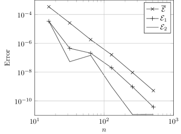
Figure 1. The true error and the error bound for evaluating at the money options for the VG model test case.

Table 1 presents the specific parameters and compares the bound for the VG model with the results obtained by Lee (2004). Based on the table, we note that for the VG model presented in Madan et al. (1998) we can achieve comparable or better error bounds when compared to the study by Lee.

To evaluate the bound, we perform the integration of (27) and (48) by relying on the Clenshaw-Curtis quadrature method provided in the SciPy package. To supplement Table 1 for a wide range of $n$, we present the magnitude of the bound compared to the true error in Figure 1.

In Figure 1, we see that the choice of numerical parameters for the Fourier inversion has a strong influence on the error of the numerical method. One does not in general have access to the true solution. Thus, the parameters need to be optimised with respect to the bound. Recall that $\mathcal{E}=\mathcal{E}(\alpha,\Delta\omega,a,n)$ and $\overline{\mathcal{E}}=\overline{\mathcal{E}}(\alpha,\Delta\omega,n)$ denote the true and estimated errors, respectively. Keeping the number of quadrature points $n$ fixed, we let $\left({\alpha_{1},\Delta\omega_{1},a_{1}}\right)$ and $\left({\alpha_{2},\Delta\omega_{2}}\right)$ denote the minimisers of the estimated and true errors, respectively

(65) $$\left({\alpha_{1},\Delta\omega_{1},a_{1}}\right) =\mathrm{arg~{}inf}~{}\overline{\mathcal{E}}$$

(66) $$\left({\alpha_{2},\Delta\omega_{2}}\right) =\mathrm{arg~{}inf}~{}\mathcal{E}$$

We further let $\mathcal{E}_{1}$ and $\mathcal{E}_{2}$ denote the true error as a function of the parameters minimising the estimated and the true error, respectively

(67) $$\mathcal{E}_{1} =\mathcal{E}\left({\alpha_{1},\Delta\omega_{1}}\right)$$

(68) $$\mathcal{E}_{2} =\mathcal{E}\left({\alpha_{2},\Delta\omega_{2}}\right)$$

In Figure 1 we see that the true error increases by approximately an order of magnitude when optimising to the bound instead of to the true error, translating into a two-fold difference in the number of quadrature points needed for a given tolerance. The difference between ${\mathcal{E}}_{1}$ and the bound is approximately another order of magnitude and necessitates another two-fold number of quadrature points compared to the theoretical minimum.

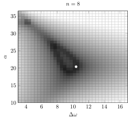
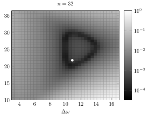
Figure 2. The true error $\mathcal{E}$ for the two VG test cases presented in Table 1 and the bound-minimising configurations (white circle) $\left({\alpha_{2},\Delta\omega_{2}}\right)$ for the examples.

In Figure 2, we present the true error for the Fourier method for the two test cases in Table 1. We note that while minimising error bounds will produce sub-optimal results, the numerical parameters that minimise the bound are a good approximation of the true optimal parameters. This, of course, is a consequence of the error bound having qualitatively similar behaviour as the true error, especially as one gets further away from the true optimal parameters.

Remark 4.1.

In practice, the Hardy norm in coefficient $M$ reduces to evaluating an $L^{1}$ norm along the two boundaries of the strip of width $2a$. We find that, for practical purposes, the performance of the Clenshaw-Curtis quadrature of the QUADPACK library provided by SciPy library is more than adequate, enabling the evaluation of the bound in a fraction of a second.

For example, the evaluations of the bounds in Table 1 take only around $0.3$ seconds to evaluate on Mid 2014 Macbook Pro equipped with a 2.6 GHz Intel Core i5 processor, this without attempting to optimize or parallelize the implementation and while checking for input sanity factors such as the evaluation of the characteristic function in a domain that is a subset in the permitted strip.

We believe that through optimizing routines, skipping sanity checks for inputs and using a lower-level computation routines this can be optimized even further, guaranteeing a fast performance even when numerous evaluations are needed.

	$K$	$80$	$90$	$100$	$110$	$120$
$12\tau=1$	$\alpha$	$-16.9$	$-13.8$	$21.6$	$29.10$	$36.3$
	$a$	$3.33$	$6.45$	$18.1$	$9.77$	$3.52$
$N=32$	$\omega_{\mathrm{\max}}$	$229$	$229$	$363$	$363$	$424$
	$\overline{\mathcal{E}}$	$3.35\times 10^{-4}$	$0.00334$	$0.00562$	$3.97\times 10^{-4}$	$7.33\times 10^{-6}$
	$\overline{\mathcal{E}}^{*}$	$6\times 10^{-4}$	$0.0032$	$0.0058$	$6\times 10^{-4}$	$1\times 10^{-4}$
$12\tau=4$	$\alpha$	$-13.8$	$-13.8$	$22.1$	$23.7$	$29.10$
	$a$	$6.11$	$6.11$	$17.9$	$15.2$	$8.75$
$N=8$	$\omega_{\mathrm{\max}}$	$62.4$	$42.4$	$84.9$	$126$	$126$
	$\overline{\mathcal{E}}$	$3.99\times 10^{-4}$	$0.00312$	$0.00398$	$3.57\times 10^{-4}$	$1.33\times 10^{-5}$
	$\overline{\mathcal{E}}^{*}$	$1.3\times 10^{-3}$	$0.0057$	$0.0055$	$9\times 10^{-4}$	$1\times 10^{-4}$

Table 1. The error bound for European call/put options in the VG model for select examples. Refererence result $\overline{\mathcal{E}}^{*}$ from Lee (2004)

Remark 4.2.

Like many other authors, we note the exceptional guaranteed accuracy of the FT-method, with only dozens of quadrature points. This is partially a result of the regularity of the European option price. Numerous Fourier-based methods have been developed for pricing path-dependent options. One might, for the sake of generality of implementation, be tempted to use these methods for European options as well, correcting for the lack of early exercise opportunities. This certainly can be done, but due to the weakened regularity, the required numbers of quadrature points are easily in the thousands, even when no rigorous bound for the error is required.

We raise one point of comparison, the the European option pricing example in Table 2 of Jackson et al. (2008), which indicates a number of quadrature points for pricing the option in the range of thousands. With the method introduced, to guarantee $\overline{\mathcal{E}}\approx 10^{-3}$, even with no optimisation, $n=64$ turns out to be sufficient.

4.2. Call options under Kou dynamics

$K$	$80$	$90$	$100$	$110$	$120$
$\overline{\mathcal{E}}$	$2.67\times 10^{-4}$	$3.49\times 10^{-4}$	$4.43\times 10^{-4}$	$5.52\times 10^{-4}$	$6.77\times 10^{-4}$
$\alpha$	$-1.57$	$-1.57$	$-1.57$	$-1.57$	$-1.57$
$\omega_{\mathrm{\max}}$	$22.9$	$22.8$	$22.6$	$22.5$	$22.4$
$\overline{\mathcal{E}}^{*}$	$0.34$	$0.26$	$0.21$	$0.17$	$0.13$
$\overline{\mathcal{E}}^{\dagger}$	$6.87\times 10^{-4}$	$1.90\times 10^{-3}$	$2.82\times 10^{-3}$	$2.72\times 10^{-3}$	$2.29\times 10^{-3}$

Table 2. Numerical performance of the bound for the Kou model, with the test case in Toivanen (2007) (see also d’Halluin et al. (2005)) with the number of quadrature points set to $n=32$. The point of comparison $\overline{\mathcal{E}}^{*}$ refers to the corresponding bound computed with the method described in Chapters $6.1$ to $6.4$ of Lee (2004). In the $\overline{\mathcal{E}}^{\dagger}$, the cutoff error has been evaluated using a computationally more intensive Clenshaw-Curtis quadrature instead of an asymptotic argument with an exponentially decaying upper bound for the option price.

For contrast with the pure-jump process presented above, we also test the performance of the bound for Kou model and present relevant results in 2. This model differs from the first example not only by being dissipative but also in regularity, in the sense that the maximal width of the domain $A_{a}$ is, for the case at hand, considerably narrower. The Lévy measure in the Kou model is given by

$$\nu_{\mathrm{Kou}}\left({\textrm{d}y}\right)=\lambda\left({pe^{-\eta_{1}y}\mathbf{1}_{y>0}+qe^{\eta_{2}y}\mathbf{1}_{y<0}}\right)$$

with $p+q=1$. For the characterisation given in Toivanen (2007) the values are set as

$$\lambda=0.1,~{}~{}r=0.05~{}~{}\tau=0.25~{}~{}S_{0}=100$$

$$p=0.3445,~{}~{}\eta_{1}=3.0465~{}~{}\eta_{2}=3.0775$$

from the expression of the characteristic exponent (see Kou and Wang (2004))

$$\Psi\left({{z}}\right)=z\left({r-\frac{\sigma^{2}}{2}-\lambda\zeta}\right)+\frac{z^{2}\sigma^{2}}{2}+\lambda\left({\frac{p\eta_{1}}{\eta_{1}-z}+\frac{q\eta_{2}}{\eta_{2}+z}-1}\right)$$

it is straightforward to see

$$A_{a}\subset\left\{{z\in\mathbb{C}:\mathrm{Im}z\in(-3.0465,3.0775)}\right\}$$

This range is considerably narrower than that considered earlier. In the case of transforming the option prices in strike space, the relevant expressions for option prices as well as the error bounds contain a factor exponential in $k$. The practical implication of this is that for deep out of the money calls, it is often beneficial to exploit the put-call-parity and to compute deep in the money calls. However, in the case at hand, the strip width does not permit such luxury. As a consequence, the parameters that minimize the bound are near-identical through a wide range of moneyness, suggesting use of FFT algorithm to evaluate the option prices at once for a range of strikes.

4.3. Binary option in the Merton model

For the particular case of Merton model, the Lévy measure is given by

$$\nu_{\mathrm{Merton}}\left({\textrm{d}y}\right)=\frac{\lambda}{\sqrt{2\pi\sigma^{2}}}\mathrm{exp}\left({-\frac{\left({y-r_{j}}\right)^{2}}{2\sigma_{j}^{2}}}\right)$$

and the characteristic exponent correspondingly by

$$\Psi\left({{z}}\right)_{\mathrm{Merton}}=z\left({r-\frac{\sigma^{2}z}{2}}\right)+\frac{\sigma^{2}z^{2}}{2}+\lambda\left({e^{zr_{j}+\frac{\sigma_{j}^{2}z^{2}}{2}}-1-z\left({e^{r_{j}+\frac{\sigma_{j}^{2}}{2}}-1}\right)}\right)$$

we may employ a fast semi-closed form evaluation of the relevant integrals instead of resorting to quadrature methods. We choose the Merton model as an example of bounding the error of the numerical method for such a model. The parameters are adopted from the estimated parameters for S&P 500 Index from Andersen and Andreasen (2000):

$$S_{0}=100,~{}~{}~{}\lambda=0.089,~{}~{}\sigma=0.1765,~{}~{}~{}r=0.05,~{}~{}r_{j}=-0.8898,~{}~{}~{}\sigma_{j}=0.4505$$

In Figure 3, we present the bound and true error for the Merton model to demonstrate the bound on another dissipative model. The option presented is a binary option with finite support on $[95,105]$; no damping was needed or used. We note that like in the case of the pure-jump module presented above, our bound reproduces the qualitative behaviour of the true error. The configuration resulting from optimising the bound is a good approximation of the true error. Such behaviour is consistent through the range of $n$ of the most practical relevance.

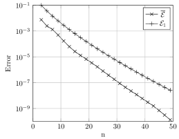
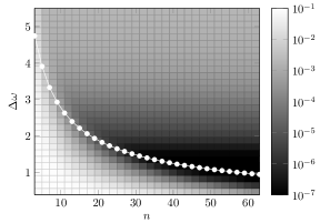
Figure 3. The true error ${\mathcal{E}}_{1}$ and the bound $\overline{\mathcal{E}}$ for the dissipative Merton model, for a range of quadrature points $n$, along with the bound-minimising configurations contrasted to the true error.

4.4. Call options

In Subsection 3.4 explicit expressions to bound $\mathcal{E}$ are provided. To evaluate these bounds it is necessary to compute $\left\|\hat{g_{\alpha}}\right\|_{L^{\infty}_{\mathbb{R}}}$ and $\left\|\hat{g_{\alpha}}\right\|_{L^{\infty}_{A_{a}}}$. According to Remark 3.9, once we compute these values we could use them for any model, provided that they satisfy the conditions considered there.

The payoff of perhaps the most practical relevance is that of a call option. Consider $g$ defined by:

$$g\left({x}\right)=\left({S_{0}e^{x}-K}\right)^{+}=S_{0}\left({e^{x}-e^{k}}\right)^{+}$$

for which a selection of a damping parameter $\alpha>0$ is necessary to have the damped payoff in $L^{1}\left({\mathbb{R}}\right)$ and to ensure the existence of a Fourier transformation. In this case we have

(69) $$\hat{g_{\alpha}}\left({\omega}\right) =S_{0}\int_{\mathbb{R}}\mathrm{exp}\left({\left({1-\alpha+i\omega}\right)x}\right)-\mathrm{exp}\left({k+\left({i\omega-\alpha}\right)x}\right)\textrm{d}x$$

(70) $$=\frac{S_{0}\mathrm{exp}\left({\left({1-\alpha+i\omega}\right)k}\right)}{\left({1+i\omega-\alpha}\right)\left({i\omega-\alpha}\right)}$$

and

(71) $$\left|{\hat{g_{\alpha}}(\omega)}\right|^{2}=\frac{S_{0}^{2}e^{2\left({1-\alpha}\right)k}}{\left({\alpha^{2}+\omega^{2}}\right)\left({\left({1-\alpha}\right)^{2}+\omega^{2}}\right)}$$

It is easy to see that the previous expression decreases as $|\omega|$ increase. This yields

(72) $$\left\|\hat{g_{\alpha}}\right\|_{L^{\infty}_{\mathbb{R}}}=\left|{\hat{g_{\alpha}}(0)}\right|=\frac{S_{0}e^{\left({1-\alpha}\right)k}}{\alpha^{2}-\alpha}$$

and

(73) $$\left\|\hat{g_{\alpha}}\right\|_{L^{\infty}_{[\varsigma,\infty)}}=\left|{\hat{g_{\alpha}}(\varsigma)}\right|$$

The maximisation of $\left|{\hat{g_{\alpha}}}\right|$ in the strip $A_{a}$ of the complex plane is more subtle. Denoting $\hat{g_{\alpha}}(\eta,\rho)=\hat{g_{\alpha}}(\eta+i\rho)$, we look for critical points that satisfy $\partial_{\eta}\left|{\hat{g_{\alpha}}}\right|=0$. This gives

(74) $$4\eta^{3}+2\eta\left({4\rho\alpha+2\alpha^{2}-2\rho-2\alpha+\rho^{2}+1}\right)=0.$$

For $\rho$ fixed, $\left|{\hat{g_{\alpha}}}\right|$ has a vanishing derivative with respect to $\eta$ at a maximum of three points. Of the three roots of the derivative, only the one characterised by $\eta=0$ is a local maximum, giving us that for call options

(75) $$\left\|\hat{g_{\alpha}}\right\|_{L^{\infty}_{A_{a}}}=\sup_{\rho\in[-a,a]}\left|{\hat{g_{\alpha}}(0,\rho)}\right|$$

Now, observe that $\left|{\hat{g_{\alpha}}(0,\rho)}\right|$ is a differentiable real function of $\rho$, whose derivative is given by the following polynomial of second degree:

(76) $$p\left({\rho}\right)\equiv k\left({\rho+\alpha-2\rho\alpha-\alpha^{2}-\rho^{2}}\right)-2\alpha-2\rho+1$$

We conclude that

(77) $$\left\|\hat{g_{\alpha}}\right\|_{L^{\infty}_{A_{a}}}=\max_{\rho\in B}\left\{\left|{\hat{g_{\alpha}}(0,\rho)}\right|\right\}$$

where $B$ is the set of no more than four elements consisting of $a$; $-a$; and the real roots of $p$ that fall in $(-a,a)$.

Remark 4.3.

So far, we have assumed the number of quadrature points $n$ to be constant. In real life applications, however, this is often not the case. Typically the user might want to choose a minimal $n$ that is sufficient to guarantee error that lies within a pre-defined error tolerance.

In such a case, we propose the following, very simplistic scheme for optimising numerical parameters and choosing the appropriate $n$ to satisfy error smaller than $\epsilon$:

1. Select $n=n_{0}$ and optimize to find the relevant configuration

2. See if $\mathcal{E_{Q}}+\mathcal{E_{F}}<\epsilon$, if not, increase $n$ by choosing it from a pre-determined increasing sequence $n=n_{j}$ and repeat procedure.

Especially in using FFT algorithms to evaluate the Fourier transforms, we propose $n_{j}=2^{j}n_{0}$. We further note that typically the optimal configuration for the optimizing configuration for $n_{j+1}$ quadrature points does not differ too dramatically from the configuration that optimizes bounds for $n_{j}$.

5. Conclusion

We have presented a decomposition of the error committed in the numerical evaluation of the inverse Fourier transform needed in asset pricing for exponential Lévy models into truncation and quadrature errors. For a wide class of exponential Lévy models, we have presented an $L^{\infty}$-bound for the error.

The error bound differs from the earlier work presented in Lee (2004) in the sense that it does not rely on the asymptotic behaviour of the option payoff at extreme strikes or option prices, allowing pricing a wide variety of non-standard payoff functions such as the ones in Suh and Zapatero (2008). The bound, however, does not take into account path-dependent options. We argue that the error for the methods that allow evaluating american, bermudan, or knockoff options are considerably more cumbersome and produce significantly larger errors so that in implementations where performance is important, such as calibration, using American option pricing methods for European options is not justified.

The bound also provides a general framework in which the truncation error is evaluated using a quadrature method that remains invariant regardless of the asymptotic behaviour of the option price function. The structure of the bound allows for a modular implementation that decomposes the error components arising from the dynamics of the system and the payoff into a product form for a large class of models, including all dissipative models. On select examples, we also demonstrate the performance that is comparable or superior to the relevant points of comparison.

We have focused on the minimization of the bound as a proxy for minimizing numerical error. Doing this, one obtains, for a given parametrization of a model, a rigorous $L^{\infty}$ bound for the error committed in solving the European option price. We have shown that the bound reproduces the qualitative behaviour of the actual error. This supports the argument for selecting numerical parameters in a way that minimizes the bound, giving evidence that this selection will, besides guaranteeing numerical precision, be close to the actual minimizing configuration that is not often achievable at an acceptable computational cost.

The bound can be used in the primitive setting of establishing a strict error bound for the numerical estimation of option prices for a given set of physical and numerical parameters or as a part of a numerical scheme, whereby the end user wishes to estimate an option price either on a single point or in a domain up to a predetermined error tolerance.

In the future, the error bounds presented can be used in efforts requiring multiple evaluations of Fourier transformations. Examples of such applications include multi-dimensional Fourier transformations, possibly in sparse tensor grids, as well as time-stepping algorithms for American and Bermudan options. Such applications are sensitive towards the error bound being used, as any numerical scheme will be required to run multiple times, either in high dimension or for multiple time steps (or both).

6. Acknowledgements

Häppölä, Crocce are members and Tempone is the director KAUST Strategic Research Initiative for Uncertainty quantification.

We wish to thank an anonymous referee for their critique that significantly improved the quality of the manuscript.

7. Declarations of Interest

The authors report no conflicts of interest. The authors alone are responsible for the content and writing of the paper.

Appendix A Truncation bound in Lee’s scheme

For the strike-space transformed option price we have

$$\tilde{f}_{\alpha}\left({\omega}\right)=\frac{\varphi_{1}\left({{\omega-i\left({\alpha+1}\right)}}\right)}{\left({i\omega+\alpha}\right)\left({i\omega+\alpha+1}\right)}$$

In the particular case of the Kou model, we have

$$\varphi_{1}\left({{\omega}}\right)=e^{\tau\left({i\omega\left({r-\frac{\sigma^{2}}{2}-\lambda\zeta}\right)-\frac{\omega^{2}\sigma^{2}}{2}+\lambda\left({\frac{p\eta_{1}}{\eta_{1}-i\omega}+\frac{q\eta_{2}}{\eta_{2}+i\omega}-1}\right)}\right)}$$

Thus,

$$\left|{\varphi_{1}\left({{\omega}}\right)}\right|=e^{\tau\left({\left({\alpha+1}\right)\left({r-\frac{\sigma^{2}}{2}-\lambda\zeta}\right)+\frac{\left({\alpha+1}\right)^{2}-\omega^{2}}{2}}\right)}e^{\tau\lambda\mathrm{Re}\left({\frac{p\eta_{1}}{\eta_{1}-\alpha-1-i\omega}\frac{q\eta_{2}}{\eta_{2}+\alpha+1+i\omega}-1}\right)}$$

We bound the first jump term resulting from upward jumps as

$$\frac{p\eta_{1}}{\eta_{1}-\alpha-1-i\omega}=\frac{p\eta_{1}\left({\eta_{1}-\alpha-1+i\omega}\right)}{\left({\eta_{1}-\alpha-1}\right)^{2}+\omega^{2}}$$

from which it follows

$$\mathrm{Re}\left({\frac{p\eta_{1}}{\eta_{1}-\alpha-1-i\omega}}\right)\leq\frac{p\eta_{1}\left({\eta_{1}-\alpha-1}\right)}{\left({\eta_{1}-\alpha-1}\right)^{2}}$$

similar inequality holds for the term resulting from downward jumps giving us that

$$\left|{\varphi_{1}\left({{\omega}}\right)}\right|\leq e^{\tau\left({\left({\alpha+1}\right)\left({r-\frac{\sigma^{2}}{2}-\lambda\zeta}\right)+\frac{\sigma^{2}\left({\alpha+1}\right)^{2}-\sigma^{2}\omega^{2}}{2}}\right)}e^{\tau\lambda\left({\frac{p\eta_{1}\left({\eta_{1}-\alpha-1}\right)}{\left({\eta_{1}-\alpha-1}\right)^{2}}+\frac{q\eta_{2}\left({\eta_{2}+\alpha+1}\right)}{\left({\eta_{2}+\alpha+1}\right)^{2}}+1}\right)}$$

The term $\mathrm{exp}\left({-\frac{\omega^{2}}{2}}\right)$ can be bounded from above by an exponential term $\mathrm{exp}\left({-\gamma\omega}\right)$:

(78) $$\mathrm{exp}\left({-\frac{\sigma^{2}\omega^{2}}{2}}\right) \leq\mathrm{exp}\left({-\gamma\omega+K}\right)$$

$$-\sigma^{2}\omega^{2}+2\gamma\omega-2K \leq 0$$

the condition for the quadratic to have no solutions is given by

$$\gamma^{2}-2K\sigma^{2}\leq 0,$$

setting $K=\frac{1}{2}$, $\gamma=\sigma$ giving us the bound in eq. (78).

This puts us in place to apply theorem 6.1 of Lee (2004), with

$$\Phi\left({u}\right) =\frac{\mathrm{exp}\left({\tau\left({\left({\alpha+1}\right)\left({r-\frac{\sigma^{2}}{2}-\lambda\zeta}\right)+\frac{\sigma^{2}\left({\alpha+1}\right)^{2}}{2}}\right)}\right)e^{\tau\lambda\left({\frac{p\eta_{1}\left({\eta_{1}-\alpha-1}\right)}{\left({\eta_{1}-\alpha-1}\right)^{2}}+\frac{q\eta_{2}\left({\eta_{2}+\alpha+1}\right)}{\left({\eta_{2}+\alpha+1}\right)^{2}}+1}\right)}}{\alpha^{2}\left({\alpha+1}\right)^{2}}$$

$$\gamma =\sigma$$

References

• (1)
• Almendral and Oosterlee (2005) Almendral, A. and Oosterlee, C. W. (2005), ‘Numerical valuation of options with jumps in the underlying’, Applied Numerical Mathematics 53(1), 1–18.
• Andersen and Andreasen (2000) Andersen, L. and Andreasen, J. (2000), ‘Jump-diffusion processes: Volatility smile fitting and numerical methods for option pricing’, Review of Derivatives Research 4(3), 231–262.
• Applebaum (2004) Applebaum, D. (2004), ‘Lévy processes and stochastic calculus, volume 93 of cambridge studies in advanced mathematics’, Cambridge, UK .
• Barndorff-Nielsen (1997) Barndorff-Nielsen, O. E. (1997), ‘Normal inverse gaussian distributions and stochastic volatility modelling’, Scandinavian Journal of statistics 24(1), 1–13.
• Black and Scholes (1973) Black, F. and Scholes, M. (1973), ‘The pricing of options and corporate liabilities’, The journal of political economy pp. 637–654.
• Boyarchenko and Levendorskii (2011) Boyarchenko, S. and Levendorskii, S. (2011), ‘New efficient versions of fourier transform method in applications to option pricing’, Available at SSRN 1846633 .
• Boyarchenko and Levendorskiǐ (2002) Boyarchenko, S. and Levendorskiǐ, S. (2002), ‘Barrier options and touch-and-out options under regular lévy processes of exponential type’, Annals of Applied Probability pp. 1261–1298.
• Briani et al. (2004) Briani, M., Chioma, C. L. and Natalini, R. (2004), ‘Convergence of numerical schemes for viscosity solutions to integro-differential degenerate parabolic problems arising in financial theory’, Numerische Mathematik 98(4), 607–646.
• Carr et al. (2002) Carr, P., Geman, H., Madan, D. B. and Yor, M. (2002), ‘The fine structure of asset returns: An empirical investigation’, The Journal of Business 75(2), pp. 305–333.
• Carr et al. (2003) Carr, P., Geman, H., Madan, D. B. and Yor, M. (2003), ‘Stochastic volatility for lévy processes’, Mathematical Finance 13(3), 345–382.
• Cont and Tankov (2004) Cont, R. and Tankov, P. (2004), Financial modelling with jump processes, Chapman & Hall/CRC Financial Mathematics Series, Chapman & Hall/CRC, Boca Raton, FL.
• De Innocentis and Levendorskii (2014) De Innocentis, M. and Levendorskii, S. (2014), ‘Pricing discrete barrier options and credit default swaps under lévy processes’, Quantitative Finance 14(8), 1337–1365.
• d’Halluin et al. (2005) d’Halluin, Y., Forsyth, P. A. and Vetzal, K. R. (2005), ‘Robust numerical methods for contingent claims under jump diffusion processes’, IMA Journal of Numerical Analysis 25(1), 87–112.
• Dotsis et al. (2007) Dotsis, G., Psychoyios, D. and Skiadopoulos, G. (2007), ‘An empirical comparison of continuous-time models of implied volatility indices’, Journal of Banking & Finance 31(12), 3584 – 3603.
• Dupire (1997) Dupire, B. (1997), Pricing and hedging with smiles, Mathematics of derivative securities. Dempster and Pliska eds., Cambridge Uni. Press.
• d’Halluin et al. (2004) d’Halluin, Y., Forsyth, P. A. and Labahn, G. (2004), ‘A penalty method for american options with jump diffusion processes’, Numerische Mathematik 97(2), 321–352.
• Eberlein (2001) Eberlein, E. (2001), Application of generalized hyperbolic lévy motions to finance, in ‘Lévy processes’, Springer, pp. 319–336.
• Feng and Linetsky (2008) Feng, L. and Linetsky, V. (2008), ‘Pricing discretely monitored barrier options and defaultable bonds in levy process models: A fast hilbert transform approach’, Mathematical Finance 18(3), 337–384.
• Hurd and Zhou (2010) Hurd, T. R. and Zhou, Z. (2010), ‘A fourier transform method for spread option pricing’, SIAM Journal on Financial Mathematics 1(1), 142–157.
• Jackson et al. (2008) Jackson, K. R., Jaimungal, S. and Surkov, V. (2008), ‘Fourier space time-stepping for option pricing with lévy models’, Journal of Computational Finance 12(2), 1.
• Kiessling and Tempone (2011) Kiessling, J. and Tempone, R. (2011), ‘Diffusion approximation of lévy processes with a view towards finance’, Monte Carlo Methods and Applications 17(1), 11–45.
• Kou (2002) Kou, S. G. (2002), ‘A jump-diffusion model for option pricing’, Management science 48(8), 1086–1101.
• Kou and Wang (2004) Kou, S. G. and Wang, H. (2004), ‘Option pricing under a double exponential jump diffusion model’, Management science 50(9), 1178–1192.
• Lee (2004) Lee, R. W. (2004), ‘Option pricing by transform methods: extensions, unification and error control’, Journal of Computational Finance 7(3), 51–86.
• Lord et al. (2008) Lord, R., Fang, F., Bervoets, F. and Oosterlee, C. W. (2008), ‘A fast and accurate fft-based method for pricing early-exercise options under lévy processes’, SIAM Journal on Scientific Computing 30(4), 1678–1705.
• Madan et al. (1998) Madan, D. B., Carr, P. P. and Chang, E. C. (1998), ‘The variance gamma process and option pricing’, European finance review 2(1), 79–105.
• Madan and Seneta (1990) Madan, D. B. and Seneta, E. (1990), ‘The variance gamma (vg) model for share market returns’, Journal of business pp. 511–524.
• Mattner (2001) Mattner, L. (2001), ‘Complex differentiation under the integral’, NIEUW ARCHIEF VOOR WISKUNDE 2, 32–35.
• Merton (1976) Merton, R. C. (1976), ‘Option pricing when underlying stock returns are discontinuous’, Journal of Financial Economics 3(12), 125 – 144.
• Nualart et al. (2001) Nualart, D., Schoutens, W. et al. (2001), ‘Backward stochastic differential equations and feynman-kac formula for lévy processes, with applications in finance’, Bernoulli 7(5), 761–776.
• Raible (2000) Raible, S. (2000), Lévy processes in finance: Theory, numerics, and empirical facts, PhD thesis, PhD thesis, Universität Freiburg i. Br.
• Reed and Simon (1975) Reed, M. and Simon, B. (1975), Methods of Modern Mathematical Physics: Vol.: 2.: Fourier Analysis, Self-Adjointness, Academic Press.
• Rydberg (1997) Rydberg, T. H. (1997), ‘The normal inverse gaussian lévy process: simulation and approximation’, Communications in statistics. Stochastic models 13(4), 887–910.
• Schmelzle (2010) Schmelzle, M. (2010), ‘Option pricing formulae using fourier transform: Theory and application’, Unpublished Manuscript .
• Stenger (1993) Stenger, F. (1993), ‘Numerical methods based on sinc and analytic functions’.
• Suh and Zapatero (2008) Suh, S. and Zapatero, F. (2008), ‘A class of quadratic options for exchange rate stabilization’, Journal of Economic Dynamics and Control 32(11), 3478–3501.
• Tankov (2004) Tankov, P. (2004), Financial modelling with jump processes, CRC Press.
• Toivanen (2007) Toivanen, J. (2007), ‘Numerical valuation of options under kou’s model’, PAMM 7(1), 1024001–1024002.